Effects of Land Use Characteristics, Physiochemical Variables, and River Connectivity on Fish Assemblages in a Lowland Basin

Abstract

Human disturbances can have severe environmental impacts on freshwater ecosystems. The main aim of this study is to detect the influences of physiochemical variables, land-cover characteristics, and river connectivity on fish assemblages in the Lake Chaohu Basin, China. A cluster analysis of river connectivity variables identified four groups of sites characterized by significantly different connectivity gradients at a local scale. These four groups of sites showed increasing connectivity from the upper reaches to the lower reaches. At the same time, among the four groups, the values of environmental variables generally increased from the upper reaches with less human activities towards the lower reaches with more human activities. For instance, some main physiochemical variables (e.g., river width, water depth, nitrate, phosphate) significantly increased among the four groups. In contrast, fish taxa richness and diversity indices were not significantly different among the four connectivity groups. However, fish assemblages showed significant variations among the connectivity groups (p = 0.026). In addition, the study determined that upper riparian land uses (e.g., woodland and grassland), flow velocity, and elevation were environmental variables regulating the variance of fish communities. As for the connectivity variables, only river order and the number of branches along a path to the left of the main stem affected the variance of fish communities. Therefore, new practices aimed at maintaining and even increasing riparian canopy coverage and the flow velocity of rivers should be integrated into local conservation planning for freshwater ecosystems, especially in the upper reaches of the basin.

1. Introduction

The species composition, abundance, and distribution of fish assemblages can be affected by both natural conditions and human activities along the spatial gradients of rivers (e.g., upper to lower reaches) [1,2,3,4]. Many natural factors caused by elevation gradients, such as temperature, precipitation, and flow velocity, co-determine species richness and distribution patterns [5,6,7,8,9]. For instance, elevation and several physiochemical variables (e.g., water depth, river width, flow velocity, and conductivity) are variables that most affect fish distribution within the Ivinhema River Basin [10]. However, some studies have found that water temperature is one of the most important natural factors influencing fish growth and production [11], which also determines how many fish species can live and grow in a given area [6]. In addition, elevation, basin area, and longitudinal river gradients primarily determine fish assemblages [9,12,13,14,15,16].

Anthropogenic disturbances (e.g., land use changes, pollutant emissions) can also influence fish assemblages [17,18,19,20,21]. Excessive nutrient input and habitat degradation derived from land use changes (e.g., changes from woodland to cropland and/or built-up land) can reduce the species richness and diversity of fish communities [14,22,23,24,25,26,27,28]. Dam construction is considered a major threat to the biodiversity of aquatic organisms because dams can alter the migratory patterns of species, influence their distribution, and block the ecological processes of natural rivers [2,4,29,30]. For instance, the construction of the Gezhou Dam led to significant losses of several endemic fish species in the Yangtze River because the dam prevented their upstream pathway of migration and substantially decreased their breeding grounds [31]. Although a large number of studies have tried to determine the factor with the greatest influence on fish assemblages, the relative importance of isolated and combined effects of natural conditions and anthropogenic disturbances on freshwater fish still needs to be determined for different regions, as these factors are characterized by a range of spatial and temporal scales [17,32,33].

Recently, numerous studies have focused on the influences of the loss of connectivity and the fragmentation of habitats generally caused by dam construction and land use changes on fish assemblages [2,8,18,26,34,35]. One of the main reasons for this focus is that many connectivity-related variables are the most important factors affecting freshwater fish assemblages in rivers [1,2,17,19,36,37]. River connectivity, referred to as hydrologic connectivity, can be defined as the water-mediated transport of matter, energy, and/or organisms within or between elements of the hydrologic cycle [19,20,21,38]. Therefore, river connectivity has an important influence on the variance among freshwater fish species. For instance, the connectivity of lakes, which is correlated with lake size, depth, and distance from rivers, is crucial in structuring fish assemblages in fluvial lakes of the Mississippi River [39]. Although very important to the contribution of connectivity-related variables to fish distribution, the combined influence of natural conditions and human activities has been proposed to be more important than the isolated influences of losses of connectivity on freshwater fish species distributions [8,14,40].

Generally, fish assemblages are likely to be affected by many factors. However, in this study, we focused on river connectivity, land use, and some common physicochemical factors. Therefore, the aims of this study were to test the hypothesis that connectivity variables regulate fish assemblages and if not, to determine which variables do regulate fish assemblages. Moreover, we tried to identify the key influential variables that currently structure fish assemblages in a lowland basin in China (the Lake Chaohu Basin) and to determine which factor is most important.

2. Materials and Methodst

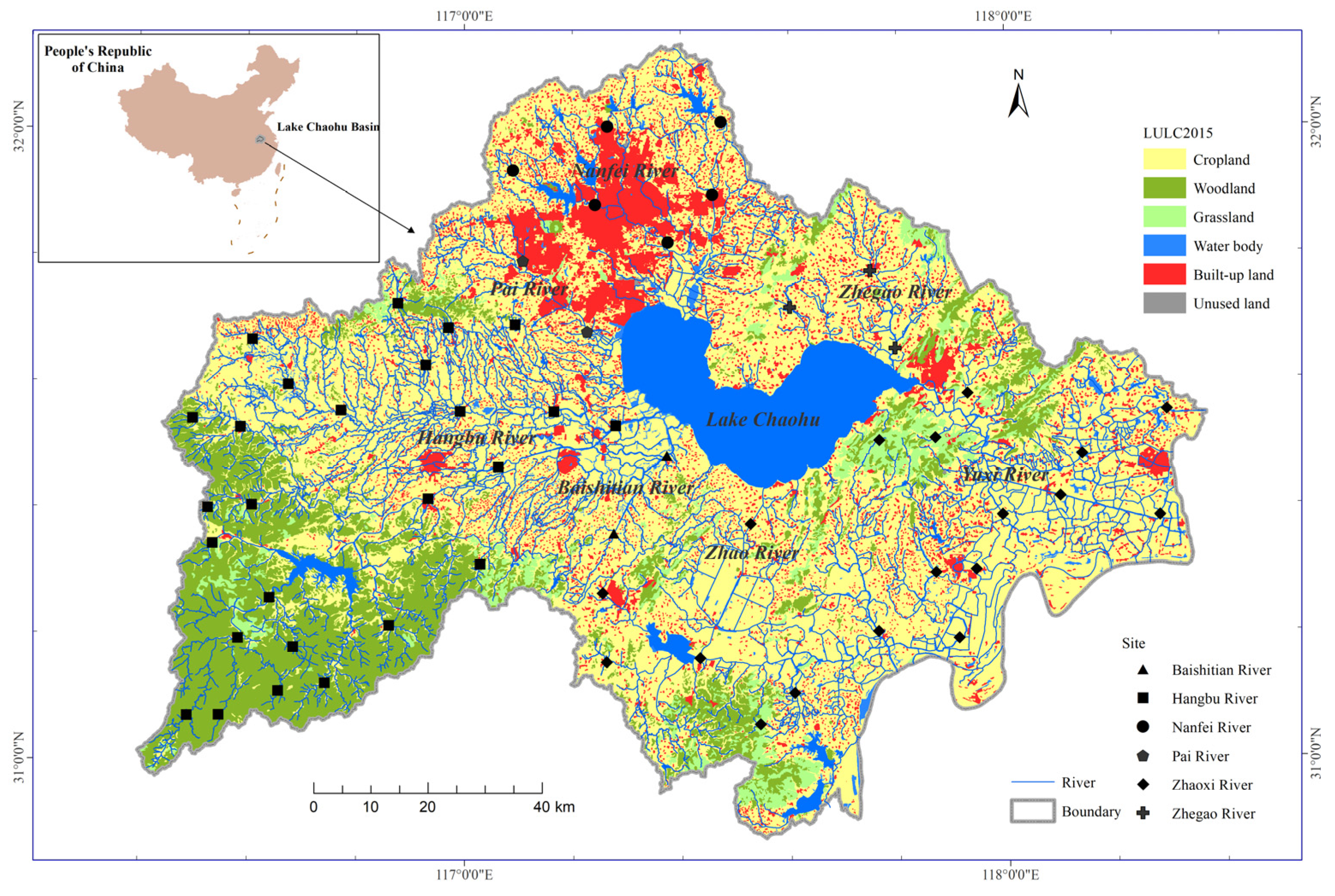
2.1. Study Area

The Lake Chaohu Basin is located in the lower reaches of the Yangtze River, with an area of 1.41 × 10⁴ km² (Figure 1). The average elevation across this area is approximately 65 m and ranges from 0 to 1498 m (higher in the west and lower in the east). More than 70% of the total area is a lowland plain, with elevations ranging from 0 to 50 m [41]. Woodland is the main land use type in the western mountains, and cropland is the main land use type in the eastern plains (Figure 1). Generally, the most prevalent land use type in the Lake Chaohu Basin is cropland (60.1% of the total area), followed by woodland (15.2%), built-up land (11.8%), water bodies (8.7%), and grassland (4.2%) in 2015.

There is a high-density river network with more than 33 rivers centripetally distributed around Lake Chaohu [41]. Most of the inflow comes from the Hangbu River, Baishitian River, and Nanfei River into Lake Chaohu [13]. However, only one river, the Yuxi River, links the lake to the Yangtze River [41]. The Hangbu River has the highest drainage density, followed by the Baishitian River, Zhaoxi River (including the Zhao River and Yuxi River), Pai River, Nanfei River, and Zhegao River [41].

2.2. Fish Sampling and Diversity Indices

During April 2013, fish were collected using a backpack electro-fishing unit (CWB-2000 p, China; 12-V import, 250-V export) by wading in two passes [42]. The sampling sites were distributed across all six main subcatchments (Hangbu River, Baishitian River, Zhaoxi River, Pai River, Nanfei River, and Zhegao River) in the Lake Chaohu basin. The sampling encompassed complete sets of characteristic segment forms (e.g., stream, pools, and riffles) [43,44]. A total of 57 sampling sites were surveyed in this study (Figure 1). A free-flowing segment of 50 m in length was sampled for each sampling site; the entire segment was sampled when it was less than 50 m in length. When the water depth was 1 m, we directly waded into the water for sampling; when the water depth was greater than 1 m, we used a rubber boat for sampling. All electro-fishing passes were conducted using uniform sampling effort, with approximately 30 min of sampling time for each 50 m segment performed by the same three persons [42]. All fish caught in the 40 m blocked segment were stored in nets which were placed in the segment to keep the fish as alive as possible. Then, the fish were identified to the lowest practical level (usually the species level), counted, and returned together to the sampling sites if alive. Unidentifiable specimens were fixed in 10% formalin and transferred to 75% ethanol for identification in the laboratory, according to additional characteristics [2].

In this study, diversity, dominance, richness, and evenness indices of fish were considered to analyze the influence of hydrological connectivity on fish α diversity. Therefore, four commonly used indices: Shannon—Wiener index, Berger—Parker dominance index, Margalef’s richness index, and Buzas and Gibson’s evenness, were calculated for each site based on species abundance data [45]. Species with a total percentage abundance of less than 0.5% were excluded from the analysis to reduce possible biases [46]. The diversity indices can be calculated as follows:

$$H=\sum _{\mathrm{i}}\left(n_i/N\right)\times \mathrm{l}\mathrm{n}\left(n_i/N\right)$$

(1)

$$BP=N_{max}/N$$

(2)

$$R=(S-1)/\mathrm{l}\mathrm{n}\left(N\right)$$

(3)

$$BG=e^H/S$$

(4)

where H, BP, R, and BG are the Shannon—Wiener index, Berger—Parker dominance index, Margalef’s richness index, and Buzas and Gibson’s evenness, respectively. n_i is the number of individuals of the ith species, and N is the total number of individuals. N_max is the number of individuals of the dominant species. S is the number of taxa.

2.3. Measured Environmental Variables

2.3.1. Local-Scale Physiochemical Variables

For each sampling site, a set of physiochemical variables was surveyed during the sampling period. The river width (Width) at each site was recorded in situ using a laser rangefinder (SNDWAY SW-1500A, SNDWAY Co., Ltd., Dongguan, China). Elevation at each site was extracted from a digital elevation model (30 m resolution), potentially available at the Resources and Environmental Science and Data Center Sciences (RESDC) at the Chinese Academy of Sciences (http://www.resdc.cn, accessed on 23 May 2023), using ArcGIS 10.1 (Environmental Systems Research Institute, Redlands, CA, USA). Flow velocity (Flow) was measured in situ by a portable, propeller-type current meter (LS300-A, Weifang Jinshui Huayu Information Technology Co., Ltd., Weifang, China). Water temperature (Temp), pH, dissolved oxygen (DO), electrical conductivity (EC), and turbidity (Turb) were measured in situ using a YSI 6600 V2 multi-parameter water quality sonde (Yellow Springs Instrument Company, Yellow Springs, OH, USA). Water depth (Depth) was measured in situ by a hydrologic sounding rod [47] (Chinese National Standard, GB/T 27992.1-2011). Some physiochemical variables (Flow, Temp, pH, DO, EC, Turb, and Depth) were measured along cross-stream transects at 3 to 5 m intervals (river width ≤ 25 m, 3 m intervals; river width > 25 m, 5 m intervals), with monitoring points spaced 1 m apart [44]. Each sampling site should have no less than 3 cross-stream transects. The cross-stream transects were set at places where the water flow was smooth and the water surface had no obvious slope. The monitoring point was located at 0.5 m below the surface of the water or at 1/2 the water depth. For each physiochemical variable above, the average value of all monitoring points at each sampling site was taken as the value of that sampling site.

Additionally, an integrated water sample was collected using a 1 L organic glass water sampler. All water samples were kept at 4 °C prior to the analyses. Other physicochemical factors, including total dissolved solid (TDS), alkalinity (Alka), dissolved organic carbon (DOC), total nitrogen (TN), ammonium (NH₄⁺-N), nitrate (NO₃⁻-N), total phosphorus (TP), and phosphate (PO₄³⁻-P), were measured in the laboratory according to standard methods [48] (American Public Health Association, 2012). After extracting water samples with 90% hot ethanol, Chlorophyll a (Chl-a) concentrations were detected by spectrophotometry [49].

2.3.2. Land Use Characteristics

The riparian buffer zone was used to identify the land use characteristics for the sampling site. Segments located 1 km upstream and downstream from the sampling site were used as the up-segment and down-segment, respectively. Therefore, the upstream and downstream riparian buffer zones could be confirmed by a 1 km buffer zone along the up-segment and down-segment, respectively. Land use characteristics for each riparian buffer zone were determined using the 30 m-accuracy land use datasets in the Lake Chaohu Basin (Figure 1), which included five categories: cropland, woodland, grassland, water body, and built-up land. These land use datasets were obtained from the RESDC. The percentage of each category of land use in each buffer zone was calculated using ArcGIS 10.1. Furthermore, the percentages of cropland, woodland, grassland, water body, and built-up land in the upstream riparian buffer zones are abbreviated as U_Crop, U_Wood, U_Grass, U_Water, and U_Built, respectively.

2.3.3. River Connectivity Variables

In this study, several common river connectivity variables were selected, which include river order, stream-link magnitude, branch link, confluence link, downstream link, upstream segment length, and downstream segment length. Specifically, river order (ROrder) was determined using Strahler’s method [50]. Stream-link magnitude (Link) is the number of unbranched source streams upstream of a given segment in a river network [51]. Branch link (BLink) is the number of branches along a path to the right (BLink_R) and left (BLink_L) of the main stem (i.e., BLink = BLink_R + BLink_L) [52]. Confluence link (CLink) is the number of confluences downstream from each stream segment [53]. Downstream link (DLink) is the link magnitude of the next downstream confluence [54]. Upstream-segment length (Up_L) is the distance from the nearest upstream confluence site to the sampling site in the same river segment, and downstream-segment length (Down_L) is the distance from the nearest downstream confluence site. Additionally, the location of the sampling site (LSS) in the segment is defined as the ratio of the upstream length to the total segment length (LSS = Up_L/T_L). A digital 1:50,000-scale hydrology map of the Lake Chaohu Basin was used to create the river network (Figure 1) and to calculate these river connectivity variables, which were performed using ArcGIS 10.1 software.

2.4. Statistical Analysis

For group sites with similar connectivity, Ward’s clustering method (a hierarchical cluster analysis method; for more details about this method, refer to [45]) was used [55], based on Euclidean distances as a measure of similarity, which were obtained from four connectivity variables (Link, BLink, CLink, and DLink). Clusters with Ward’s method are joined in such a way, that increases in within-group variance are minimized. This clustering can be performed using PAST 4.14 software [45].

There are three types of environmental variables: 18 local-scale physiochemical variables, 5 land use characteristics variables, and 10 river connectivity variables, in our dataset, but not all of these variables could be directly used to analyze their effects on fish diversity indices due to multicollinearity among them. Thus, it was necessary to select available variables. First, to reduce dimensionality and better compare the variables, all initial values (except for land use characteristics) were normalized using the min-max normalization method [56]. Second, a variance inflation factor (VIF) was employed to detect multicollinearity among the variables. If the VIF was more than 5, multicollinearity was likely present, and a threshold value of 5 was therefore set to decrease the effects of multicollinearity [57,58]. The VIF was calculated using the package vegan (version 2.5–7) [59] in R (R Development Core Team, 2013). Finally, to reduce the complexity of the variation partitioning analysis (VPA), the factors with a VIF < 5 within the three groups were further screened according to their relative importance, which was calculated based on the sum of their Akaike weights (SAW) in a mixed-effects meta-regression model using the glmulti package (Version 1.0.8) in R. If the SAW was more than 0.8, the parameter was considered a key driving variable for explaining the deviance in the fish diversity indices [60,61]. Key driving variables were considered good predictors of the response variable without the need to invoke other variables [61].

Furthermore, VPA was performed to disentangle the influential intensity of the key driving variables (SAW > 0.8) on the fish diversity indices [62]. This was performed using the varpart function in the vegan package (version 2.5–7) in R. The proportions of the variation in fish diversity indices that were explained by the unique and combined influences of the key driving variables were reported based on adjusted R² values [62,63]. Negative values in the report were not considered because they indicated that the explained variance might be negligible [61]. Finally, we used multiple regression analysis to detect the effects (strength and direction) of each key driving variable on the fish diversity indices, which was also performed in R.

The physiochemical variables (except for pH), land use variables, river connectivity, and species abundance data were log₁₀(x + 1) transformed before the following analysis to reduce the influence of non-normal distribution. In addition, as variances in the local-scale physiochemical variables and diversity indices were not homogeneous, the nonparametric Kruskal—Wallis test was employed to detect the differences in the local-scale physiochemical variables and diversity indices among the connectivity groups using SPSS 20.0 (IBM Co., Ltd., Chicago, IL, USA) [13].

Several statistical analysis methods were employed to test which variables regulate fish assemblages. Nonmetric multidimensional scaling (NMDS) was employed to assess the spatial variation in fish assemblages based on Bray—Curtis dissimilarity measures of fish abundance data. One-way analysis of similarity (ANOSIM) was also used to determine whether fish assemblages differed significantly among the connectivity groups [2,13]. Additionally, similarity percentage (SIMPER) procedures were employed to identify the species that contributed the most to the dissimilarities among groups [22]. These analyses were performed using PAST 3.21 software [45], accordingly.

Furthermore, to identify the key influencing variables that currently structure the fish assemblages and determine which factor was the most important, a canonical correspondence analysis (CCA) was performed based on abundance data [2]. A manual forward selection procedure was employed to identify which environmental variables were significantly related to the fish assemblages. The environmental variables with a significance level of p < 0.1 were chosen based on 9999 Monte Carlo permutation tests [13]. The explanatory power of these environmental variables in relation to the fish assemblages were calculated as the percentages of the selected variables in relation to the total explanatory power, all of which can be obtained from the forward selection step in the Canoco 4.5 software [64].

The fish abundance data were log₁₀(x + 1) transformed before the analyses to reduce the influence of non-normal distribution. Local-scale physiochemical variables (except TDS, TN, NH₄⁺-N, PO₄³⁻-P) and land use characteristics (except the proportion of cropland) were included in CCA analyses because TDS, TN, NH₄⁺-N, PO₄³⁻-P, and the proportion of cropland were multiple collinearities with other variables. Species that occurred at fewer than five sites were excluded from NMDS, ANOSIM, and CCA analyses [2].

3. Results

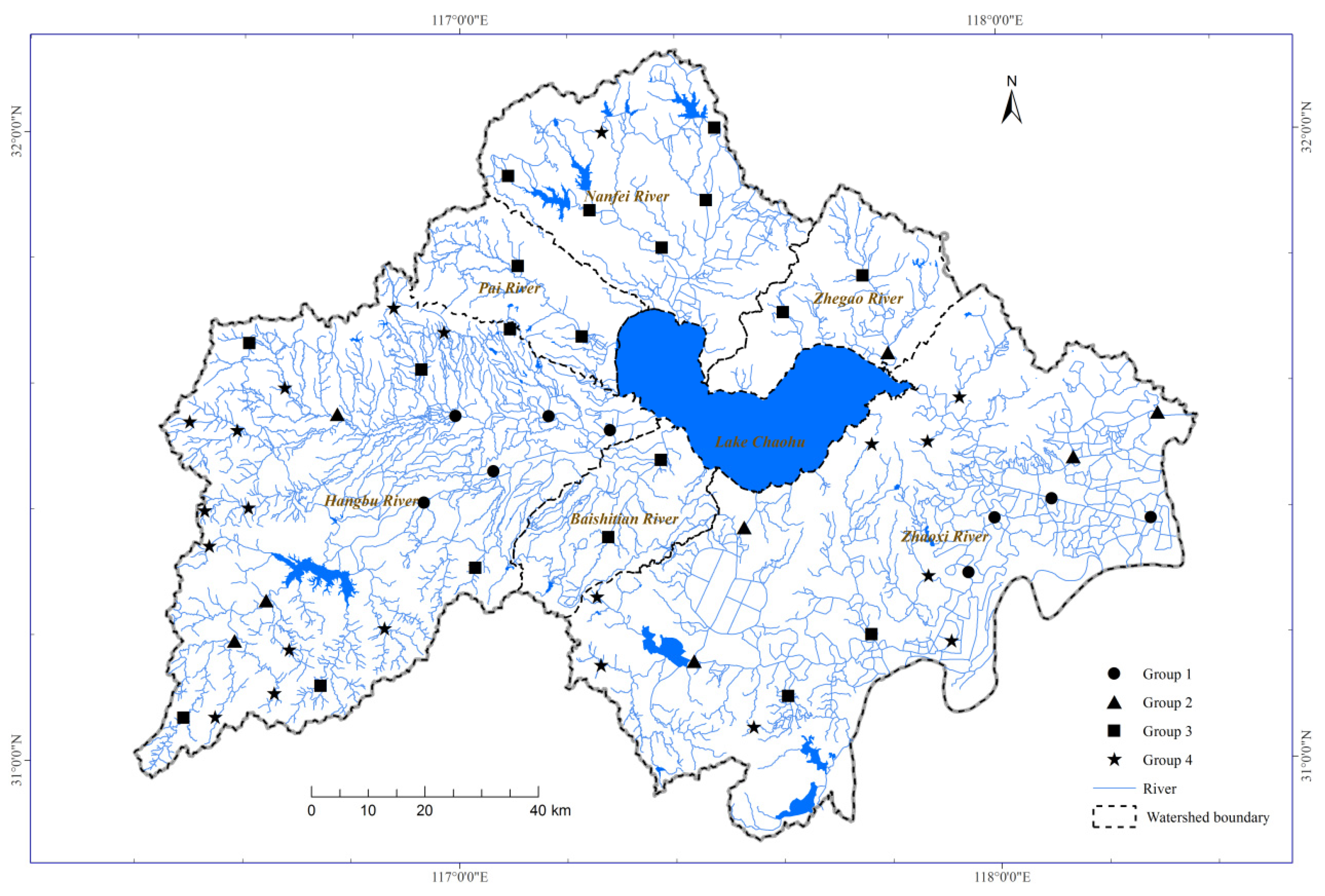
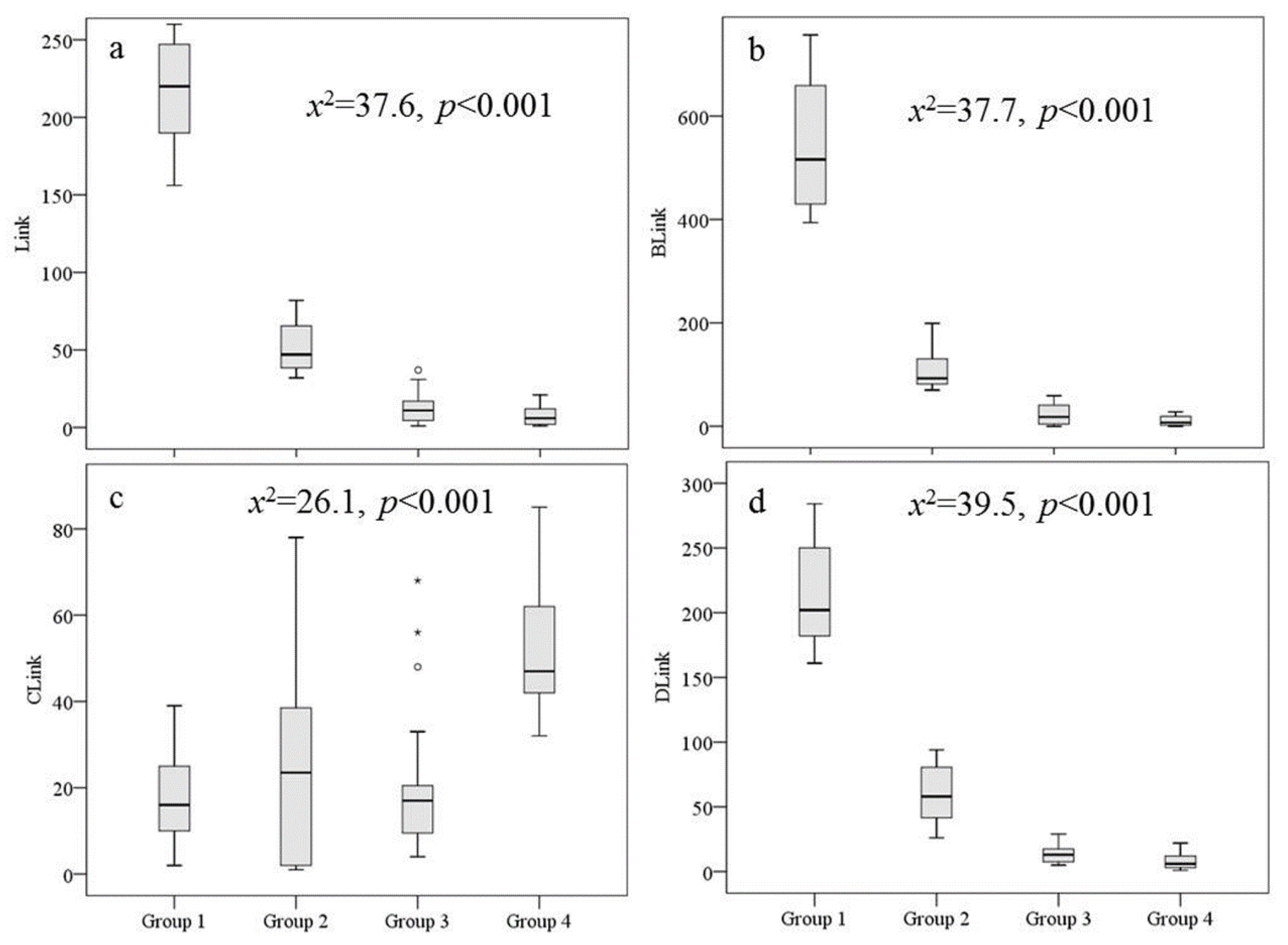
3.1. Clustering River Connectivity Variables

The cluster analysis resulted in four groups of sites with a Euclidean similarity of 200 among sites within a cluster. The sampling sites of these four groups showed an upper-lower reach distribution pattern across the basin (Figure 2). The four groups formed in the cluster analysis had significantly different connectivity, according to the Kruskal—Wallis test (Figure 3 and

Table 1. Connectivity variables for the four connectivity groups in the Lake Chaohu Basin. Kruskal—Wallis tests were conducted to detect differences in variables among groups. Values are averages (ranges).

Physicochemical Variables	River-Connectivity Group				p Value
	Group 1 (n = 9)	Group 2 (n = 8)	Group 3 (n = 19)	Group 4 (n = 21)
ROrder	4.67 (2–5)	4.13(4–5)	2.89 (1–4)	2.43 (1–3)	<0.001 ***
Link	250.22 (156–567)	52 (32–82)	12.89 (1–37)	7.38 (1–21)	<0.001 ***
BLink_Lf	279.56 (108–970)	60.38 (5–119)	13.68 (0–45)	4.95 (0–16)	<0.001 ***
BLink_R	353.22 (215–537)	49.38 (26–84)	10.21 (0–33)	5.81 (0–18)	<0.001 ***
BLink	632.78 (394–1423)	109.75 (70–199)	23.89 (0–59)	10.76 (0–28)	<0.001 ***
CLink	18 (2–39)	25.88 (1–78)	21.05 (4–68)	53.05 (32–85)	<0.001 ***
DLink	239.11 (161–499)	60 (26–94)	14.05 (5–29)	8.1 (1–22)	<0.001 ***
Down_L (km)	1290.5 (13.02–3911)	1700.35 (63.37–6957)	874.07 (10.9–7329)	2016 (11.8–16,500)	0.420
Up_L (km)	1227.53 (131.1–5231)	1504.04 (29.43–3930)	997.75 (11.48–4852)	1414.17 (13.11–4840)	0.826
LSS	0.51 (0.05–0.99)	0.55 (0.01–0.94)	0.56 (0.04–0.98)	0.46 (0.01–0.99)	0.909

*** Correlation is significant at the 0.001 level. ROrder, stream order; Link, stream-link magnitude; BLink_Lf, number of branches along a path to the left; BLink_R, number of branches along a path to the right; BLink, branch link; CLink, confluence link; DLink, downstream link; Down_L, downstream segment length; Up_L, upstream segment length; and LSS, the location of sampling site.

). For example, sites in Group 1 had the highest Link, BLink, and DLink values, followed by the sites in Groups 2, 3, and 4. However, sites in Group 4 had the highest values of CLink, followed by the sites in Groups 2, 3, and 1. Generally, these results indicated that sites in Group 1 usually had the highest connectivity from the lower to upper reaches, followed by sites in Groups 2, 3, and 4 (Figure 2 and Figure 3).

Therefore, sites from Group 1 were mainly located in the lower reaches with high-connectivity segments (e.g., Hangbu River and Zhaoxi River). Sites from Group 2 were clustered in the upper reaches with moderate-connectivity segments (e.g., Hangbu River and Zhaoxi River). Sites from Group 3 were mainly distributed in the middle reaches with low-connectivity segments (e.g., Nanfei River, Pai River, Zhegao River, and Baishitian River). Sites from Group 4 were situated in the upper reaches with the lowest connectivity segments (e.g., Nanfei River, Pai River, Zhegai River, Baishitian River, Hangbu River, and Zhaoxi River).

Generally, river orders in the Lake Chaohu Basin ranged from 1st to 5th (See ROrder in Table 1). Link, BLink_R, BLink_Lf, BLink, CLink, and DLink ranged from 1 to 567, 0 to 970, 0 to 537, 0 to 1423, 1 to 58, and 1 to 499, respectively. Upstream segment length (Up_L) and downstream segment length (Down_L) ranged from 0.01 to 5.23 km and 0.01 to 16.50 km, respectively. The location of the sampling site (LSS) ranged from 0.01 to 0.99.

3.2. Spatial Gradients of Physiochemical Variables among Connectivity Groups

Although many physiochemical variables were not significantly different among the four connectivity groups, several variables (e.g., Width, Depth, NO₃⁻-N, TP, DOC, and PO₄³⁻-P) were significantly different among the four groups according to the Kruskal—Wallis test (

Table 2. Physicochemical variables for the four connectivity groups in the Lake Chaohu Basin. The Kruskal—Wallis tests were conducted to detect differences in variables among groups. Values are averages (ranges).

Physicochemical Variables	River-Connectivity Group				p Value
	Group 1 (n = 9)	Group 2 (n = 8)	Group 3 (n = 19)	Group 4 (n = 21)
pH	8.39 (7.4–9.87)	8.22 (6.93–9.87)	8.25 (7.5–10.16)	8.06 (7.23–9.19)	0.619
DO (mg/L)	10.72 (6.14–18.22)	9.82 (3.22–18.22)	8.86 (0.85–13.45)	9.86 (1.46–16.94)	0.896
EC (μs/cm)	158.56 (69–221)	185.75 (41–323)	201.74 (33–576)	191.9 (41–616)	0.939
TDS (mg/L)	0.12 (0.05–0.17)	0.14 (0.03–0.26)	0.15 (0.03–0.4)	0.14 (0.04–0.29)	0.952
Alka (mg/L)	35.18 (0–59.36)	40.99 (14.13–62.19)	60.7 (19.79–115.89)	44.82 (8.48–132.85)	0.088
Turb (NTU)	14.22 (0.9–30.9)	8.6 (0.9–20.4)	21.78 (0.1–116.1)	10.75 (0.3–34.8)	0.414
TN (mg/L)	0.63 (0.09–2.11)	0.52 (0.08–2.11)	2.64 (0.17–15.85)	0.60 (0.09–4.99)	0.595
NH4+-N (mg/L)	0.49 (0.13–1.8)	0.76 (0.06–2.74)	0.14 (0.04–0.73)	0.21 (0.04–1.04)	0.082
NO3−-N (mg/L)	1.72 (0.66–2.7)	1.94 (0.45–4.97)	3.77 (0.57–17.87)	1.70 (0.48–5.55)	0.006 **
TP (mg/L)	0.06 (0.02–0.26)	0.05 (0.01–0.24)	0.20 (0.01–1.05)	0.03 (0–0.06)	0.013 *
PO43−-P (mg/L)	0.11 (0.04–0.34)	0.08 (0.02–0.34)	0.41 (0.02–2.66)	0.05 (0.01–0.11)	0.020 *
DOC (mg/L)	4.55 (3.03–7.59)	5.13 (3.18–7.21)	7.17 (2.34–16.81)	4.72 (1.45–8.03)	0.041 *
Elevation (m)	22 (12–33)	50.25 (18–123)	57.63 (8–387)	63.24 (7–159)	0.023 *
Temp (°C)	18.77 (15.99–25.25)	17.83 (13.32–25.25)	18.76 (10.96–25.89)	17.85 (12.3–25.23)	0.495
Width (m)	149.22 (40–320)	61.38 (10–108)	48.16 (4–240)	20.67 (3–150)	<0.001 ***
Depth (m)	4.12 (0.9–7)	2.21 (0.8–4)	1.98 (0.3–4)	0.99 (0.3–5)	<0.001 ***
Flow (m/s)	0.10 (0–0.2)	0.19 (0–0.61)	0.09 (0–0.51)	0.18 (0–0.81)	0.349
Chl-a (μg/cm2)	0.25 (0.03–0.71)	0.17 (0.05–0.33)	0.40 (0.05–1.79)	0.31 (0.02–1.27)	0.899

Note: * p < 0.05, ** p < 0.01, *** p < 0.001.

and Figure 4). Specifically, in comparison to the other sites and Groups, major sites in Group 3 had the highest pollution (e.g., EC and Turb) and nutrient levels (e.g., TN, NO₃⁻-N, TP, PO₄³⁻-P, and DOC) and the lowest values for DO, Flow, and NH₄⁺-N, whereas sites in Groups 4 and 2 had low nutrient and pollution levels and higher flow velocity. Sites in Group 1 had the highest Width, Depth, and DO, and even the highest pH values. Sites in Group 1 had the highest values of the connectivity variables (ROrder, Link, BLink, and DLink), local-size variables (river width, water depth, and DO), and U_Crop. The sites in Group 4 had the highest Elevation, U_Wood, and U_Grass; the lowest river width, water depth, and U_Crop; and the lowest nutrient levels (e.g., TP, NO₃⁻-N, PO₄³⁻-P).

There was a significant spatial gradient in the land use characteristics along the river segments (

Table 3. Land use and land cover for the four connectivity groups in the Lake Chaohu Basin. The Kruskal—Wallis tests were conducted to detect differences in variables among groups. Values are averages (ranges).

Land Use and Land Cover	River-Connectivity Group				p Value
	Group 1 (n = 9)	Group 2 (n = 8)	Group 3 (n = 19)	Group 4 (n = 21)
U_Grass	0 (0–0)	1.25 (0–9.98)	1.49 (0–28.33)	12.72 (0–86.32)	0.018 *
U_Built	9.18 (0–21.46)	9.5 (0–13.93)	21.56 (0–84.98)	7.57 (0–54.3)	0.080
U_Crop	78.21 (63.45–97.14)	66.68 (27.34–90.72)	62.83 (0–98.76)	49.64 (0–97.25)	0.127
U_Wood	1.39 (0–12.47)	15.25 (0–61.85)	10.83 (0–100)	27.52 (0–100)	0.002 **
U_Water	11.22 (0–31.16)	7.32 (0–23.31)	3.29 (0–39.3)	2.54 (0–13.58)	0.032 *
D_Grass	0 (0–0)	1.16 (0–6.84)	1.31 (0–24.96)	10.09 (0–57.22)	0.094
D_Built	8.02 (0–28.55)	9.76 (0–19.88)	19.03 (0–99.24)	8.15 (0–42.62)	0.255
D_Crop	81.04 (62.05–94.97)	66.53 (28.8–93.2)	65.81 (0–98.6)	53.95 (0–96.4)	0.081
D_Wood	0 (0–0)	12.98 (0–56.08)	10.39 (0–100)	24.87 (0–100)	0.002 **
D_Water	10.95 (0–33.17)	9.56 (0–35.79)	3.31 (0–41.23)	2.94 (0–13.15)	0.031 *
T_Grass	0 (0–0)	1.29 (0–8.33)	1.41 (0–26.81)	10.16 (0–53.22)	0.023 *
T_Built	8.44 (0–22.94)	9.78 (0–18.71)	19.89 (0–89.66)	8.07 (0–44.31)	0.179
T_Crop	79.72 (64.61–95.73)	66.37 (27.91–92.15)	64.58 (0–98.68)	52.92 (0–96.73)	0.098
T_Wood	1.1 (0–9.87)	14.44 (0–59.59)	10.7 (0–100)	26.07 (0–100)	0.001 ***
T_Water	10.75 (0–32.06)	8.12 (0–27.88)	3.37 (0–40.12)	2.78 (0–12.98)	0.045 *

Note: * p < 0.05, ** p < 0.01, *** p < 0.001. U_Grass, U_Built, U_Crop, U_Wood, and U_Water represent the grassland, built-up land, cropland, woodland, and water body in the 1 km buffer along the upstream segment where sampling site located, respectively. D_Grass, D_Built, D_Crop, D_Wood, and D_Water represent the grassland, built-up land, cropland, woodland, and water body in the 1 km buffer along the downstream segment, respectively. T_Grass, T_Built, T_Crop, T_Wood, and T_Water represent the grassland, built-up land, cropland, woodland, and water body in the 1 km buffer along the total segment, respectively.

and Figure S1). The percentage of grassland in the 1 km buffer along the upstream segments (U_Grass) decreased from the upper reach sites (Group 4) to the lower reach sites (Group 1). On the other hand, the percentage of water body in the 1 km buffer along the upstream segments (U_Water) showed the opposite trend, increasing from the upper reach sites (Group 4) to the lower reach sites (Group 1). The percentage of woodland in the 1 km buffer along the upstream segments (U_Wood) showed a complex trend along the segments, with the highest values in the upstream segments of sites in Group 4. The next highest U_Wood values were in the upstream segments of sites in Group 2, followed by Group 3 and Group 1. Although the percentage of cropland in the 1 km buffer along the upstream segments (U_Crop) and the percentage of built-up land in the 1 km buffer along the upstream segments (U_Built) were not significantly different among the four connectivity groups, U_Crop increased from the upper reach sites (Group 4) to the lower reach sites (Group 1), and the highest U_Built was clustered in Group 3. The same results were found downstream and for all segments of the sites (Table 3 and Figure S1).

3.3. Influence of River Connectivity on Fish Assemblages

A total of 2166 individuals were collected throughout the Lake Chaohu Basin at 57 sites, representing 38 species in 35 genera and 13 families. Species richness and the number of individuals caught varied from 1 to 14 and 1 to 445, respectively, across sites. Based on the Kruskal—Wallis test, fish taxa richness and diversity indices were not significantly related to all river connectivity variables (not shown in the text) and no significant difference existed among the connectivity groups (p > 0.099,

Table 4. Fish taxa richness and diversity indices in the four connectivity groups in the Lake Chaohu Basin. Kruskal—Wallis tests were conducted to detect differences in variables among groups. Values are averages (ranges).

Fish Taxa Richness and Diversity Indices	River-Connectivity Group				p Value
	Group 1 (n = 9)	Group 2 (n = 8)	Group 3 (n = 19)	Group 4 (n = 21)
Number of taxa	6.89 (3–13)	6.13 (4–11)	7.53 (1–14)	5.48 (1–12)	0.119
Total number of individuals	53.67 (12–142)	46.25 (10–110)	89.11 (1–455)	44 (1–122)	0.114
Shannon-Wiener index	0.63 (0.25–0.92)	0.7 (0.47–0.9)	0.57 (0.33–1)	0.68 (0.32–1)	0.099
Buzas and Gibson’s evenness	1.11 (0.6–1.59)	1.16 (0.67–1.77)	1.14 (0–1.71)	0.95 (0–1.9)	0.482
Margalef’s richness index	0.72 (0.42–0.95)	0.78 (0.53–0.92)	0.66 (0.29–0.82)	0.72 (0.17–0.96)	0.159
Berger-Parker dominance index	0.54 (0.29–0.83)	0.46 (0.32–0.77)	0.55 (0.29–1)	0.56 (0.19–1)	0.625

). However, fish assemblages significantly varied by connectivity groups (global R = 0.089, p = 0.026), particularly between Groups 3 and 4 and Groups 2 and 4.

However, one-way ANOSIM results showed that fish assemblages significantly varied by connectivity groups (global R = 0.089, p = 0.026). Specifically, fish assemblages could be distinguished between Groups 3 and 4 (R = 0.160, p = 0.006) and Groups 2 and 4 (R = 0.127, p = 0.048) (

Table 5. One-way ANOSIM showing significance levels of fish community structure among the four groups. The upper triangular matrix shows the p values, and the lower triangular matrix shows the global R statistic.

	Group 1	Group 2	Group 3	Group 4
Group 1		0.696	0.320	0.104
Group 2	−0.042		0.390	0.048 *
Group 3	0.029	0.004		0.006 **
Group 4	0.100	0.127	0.160

* p < 0.05, ** p < 0.01.

). The SIMPER analysis revealed that the species that primarily contributed to the dissimilarity between Groups 3 and 4 were Carassius auratus (16.72% of contribution), Ctenogobius sp. (13.14%), Hemiculter leucisculus (11.45%), and Misgurnus anguillicaudatus (8.53%), while Ctenogobius auratus (18.10%), Ctenogobius sp. (14.24%), H. leucisculus (11.41%), and Acheilognathus barbatulus (6.10%) mostly contributed to the difference between Groups 2 and 4. In addition, Carassius auratus, Ctenogobius sp., and Hemiculter leucisculus were the dominant species and occurred at most of the sites throughout the Lake Chaohu Basin. Furthermore, the minimum stress value was 0.14 in the NMDS ordination solution for the river connectivity groups (Figure 5a). The NMDS analysis revealed that sampling sites in Group 3 were mainly located on the right of the graph, while the sites in Group 4 were gathered to the left. At the same time, sampling sites in Groups 1 and 2 were mainly clustered to the top of the plot.

Based on the Kruskal—Wallis test, fish taxa richness and diversity indices were not significantly different among river order groups (

Table 6. Fish taxa richness and diversity indices in the river order groups in the Lake Chaohu Basin. Kruskal—Wallis tests were conducted to detect differences in variables among groups. Values are averages (ranges).

Fish Taxa Richness and Diversity Indices	River-Order Group					p Value
	1st-Order (n = 3)	2nd-Order (n = 14)	3rd-Order (n = 19)	4th-Order (n = 12)	5th-Order (n = 9)
Number of taxa	4.67 (3–6)	7 (1–13)	5.89 (1–10)	7.58 (4–14)	6 (3–10)	0.492
Total number of individuals	30.67 (5–55)	46.5 (1–142)	63.58 (1–122)	96.08 (10–455)	40.67 (12–92)	0.236
Shannon-Wiener index	0.78 (0.66–0.96)	0.68 (0.25–1)	0.58 (0.32–1)	0.59 (0.33–0.9)	0.7 (0.39–0.92)	0.149
Buzas and Gibson’s evenness	1.01 (0.68–1.24)	1.11 (0–1.9)	0.93 (0–1.71)	1.22 (0.67–1.77)	1.13 (0.6–1.59)	0.649
Margalef’s richness index	0.84 (0.77–0.96)	0.74 (0.46–0.93)	0.62 (0.17–0.87)	0.72 (0.53–0.92)	0.77 (0.42–0.95)	0.089
Berger-Parker dominance index	0.44 (0.4–0.5)	0.52 (0.19–1)	0.62 (0.29–1)	0.5 (0.33–0.77)	0.5 (0.29–0.83)	0.415

). Similarly, there was also no significant difference in fish assemblages among river orders (global R = 0.004, p = 0.424). Therefore, river order cannot influence fish assemblages in the Lake Chaohu Basin. However, the minimum stress value was 0.14 in the NMDS ordination solution for river orders (Figure 5b). The NMDS analysis revealed that the sampling sites in the 2nd- and 3rd-order streams were mainly located on the right of the graph, while the sampling sites in the 5th-order streams were gathered to the left. At the same time, the sampling sites in the 1st-order streams were mainly clustered to the bottom right, and the sampling sites in the 4th-order streams were mainly located at the top.

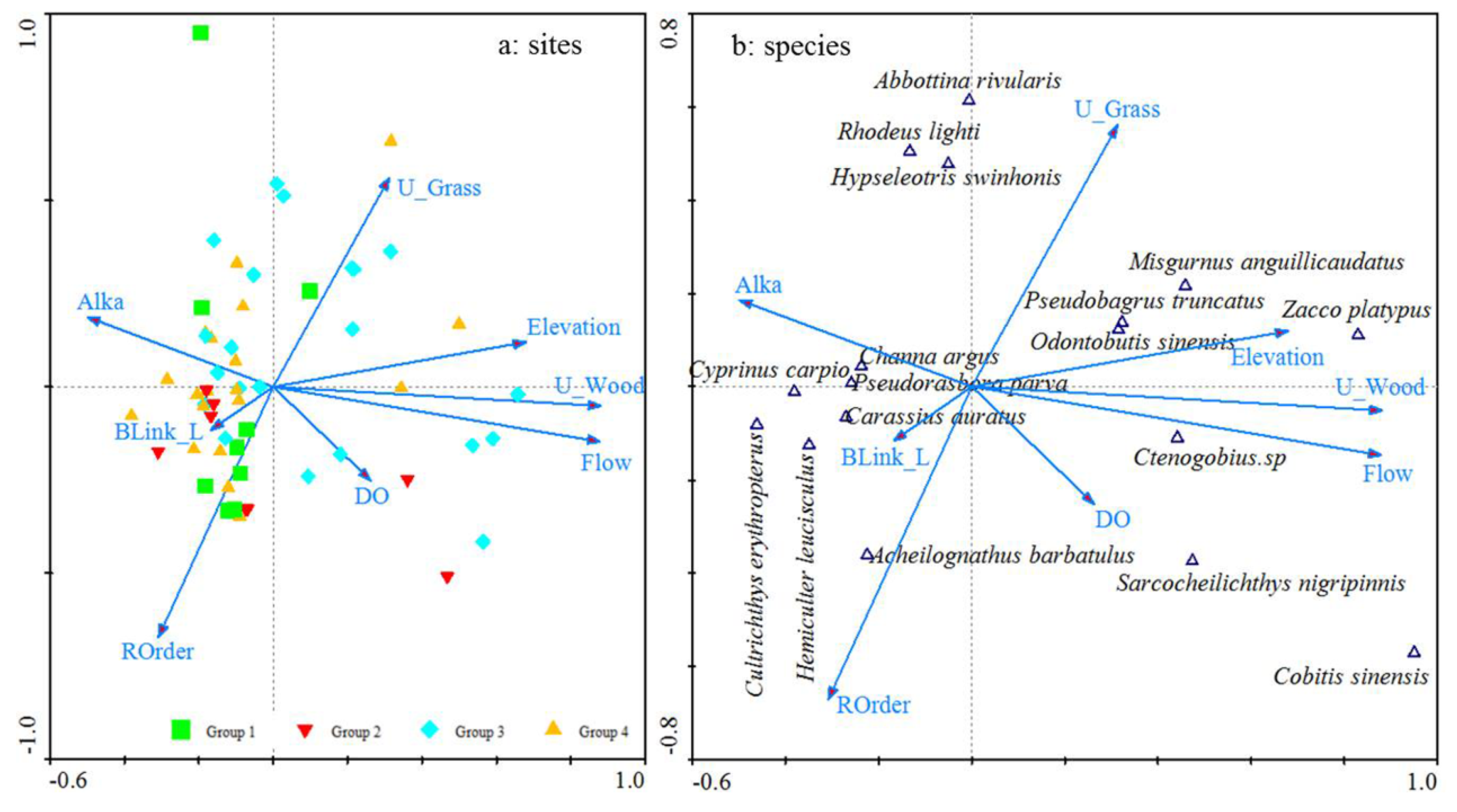
3.4. Linking Environmental Variables to Fish Assemblages

The forward selection procedure for the CCA identified eight environmental variables (U_Wood, U_Grass, Flow, ROrder, Alka, Elevation, BLink_Lf, and DO) that were highly correlated with the fish communities (Figure 6). U_Wood explained the most variance (15.4%), followed by U_Grass (5.4%), Flow (5.1%), ROrder (3.0%), Alka (2.8%), Elevation (2.7%), BLink_Lf (2.6%), and DO (2.5%). The first and second axes accounted for 16.5 and 6.8%, respectively, of the total variation in fish species abundances. The first axis was highly related to the variables U_Wood (canonical coefficient, r = 0.75), Flow (r = 0.75), and Elevation (r = 0.58), while the second axis was corrected to U_Grass (r = 0.42). In addition, the first axis was negatively related to ROrder (r = −0.50). Based on the CCA plot, many sites in the lower reaches of the high-connectivity rivers (Group 1) were clustered around ROrder, while some sites in the upper reaches of the low-connectivity rivers (Group 4) were gathered around BLink_Lf and Alka. Sites in the lower reaches of high-connectivity rivers (Group 1) were located around BLink_Lf and DO. In addition, sites in the middle reaches of low-connectivity rivers (Group 3) were plotted along Flow, U_Wood, U_Grass, and Elevation. Therefore, ROrder and BLink_Lf explain a fraction of the variance (3.0% and 2.6%, respectively).

The CCA results also showed the relationships between some common species and the eight environmental variables (Figure 6b). Two dominant species, C. auratus and H. leucisculus, were positively related to BLink_Lf and negatively related to U_Wood, Flow, and Elevation. This result means that these two species would prefer to live in the lower reaches with high BLink_Lf and low Elevation, U_Wood, and Flow. The other dominant species, Ctenogobius sp., were positively correlated with Flow, U_Wood, and Elevation. Similarly, five species (such as Zacco platypus, Misgurnus anguillicaudatus, Ctenogobius sp., Pseudobagrus truncates, and Odontobutis sinensis) were positively correlated with Elevation, U_Wood, and Flow. In other words, these species generally occurred in the upper reaches with high Elevation, U_Wood, and Flow. Moreover, Abbottina rivularis, Rhodeus lighti, and Hypseleotris swinhonis were most frequently found in the upper reaches of high U_Grass and low ROrder. Additionally, Cobitis sinensis and Sarcocheilichthys nigripinnis were found in the upper and middle reaches with high DO.

4. Discussion

4.1. Spatial Heterogeneity of Environmental Variables

Many environmental variables showed significant variation along the longitudinal gradients of the rivers throughout the Lake Chaohu Basin. Specifically, sites in Group 3 had the highest nutrient levels (e.g., TN, NO₃⁻-N, TP, and PO₄³⁻-P), which was likely because this area has the highest amount of built-up land along the segments of these sites [13,65]. Moreover, nutrient levels showed an increasing trend from sites in the upper reaches to the lower reaches (Table 2). However, due to anthropogenic disturbances such as the increase of built-up land and cropland, this increasing trend in nutrient variation can be transformed suddenly [13,14,24]. For example, sites in Group 3, which were located in the middle and lower reaches, had the highest nutrient levels. This scenario means that human activities (e.g., land use change from woodland and water bodies to built-up land and cropland) can strongly influence water quality in this region [15,24].

Moreover, in this study, a cluster analysis of the river connectivity variables identified four groups of sampling sites that were characterized by significantly different river connectivity and longitudinal gradients. This clustering is significantly different from the results of Yu et al. [55], who simply categorized the sampling sites into two groups, isolated and connected. Their study focused on the relationships between water quality in isolated and connected wetlands and their surrounding watersheds, documenting that the DOC was significantly lower in connected wetlands than in isolated wetlands when land use did not change significantly. However, this difference can be completely due to changes in land use. Furthermore, according to varying flood intensities, the sampling sites can be grouped into five categories: drought-connected, low flood-connected, moderate flood-connected, high flood-connected, and extreme flood-connected [19,66]. Research has determined that the effect of connectivity on water chemistry has shown that lakes with greater connectivity usually have higher DO and NO₃⁻-N and lower TN and TP. These different results may vary from those in our study due to variations in cluster connectivity and the different subjects under study (wetlands/lakes vs. rivers).

Similarly, some environmental variables did not show significant variation along the rivers, but several main nutrients had remarkably different concentrations among the connectivity groups. This result is also slightly different from the results of Zhang et al. [13], whose research showed that all environmental variables had significant differences among their cluster groups. Their research may have used species abundance data to cluster the sampling sites, whereas we used the four connectivity variables to cluster the sampling sites in this study, due to the aims of our research.

4.2. Connectivity Variables Slightly Influence Variations in Fish Assemblages

Due to the lack of available data on fish assemblages in the Lake Chaohu Basin, temporal variability was not detected in this study. The most significant way in which our study differs from most others is that the sampling sites were grouped according to four river connectivity variables. Thus, we focused on spatial variance in fish assemblages and tested the hypothesis that fish assemblages are regulated by river connectivity variables in the lowland basin (the Lake Chaohu Basin, China). However, the results of this study cannot support our hypothesis that river connectivity variables regulate fish assemblages. The results instead indicate that these connectivity variables can explain a small part of the variance and slightly influence the variation in fish assemblage in the lowland basin of China. In contrast, the LSS was not significantly different among river order groups (Table 1) and did not explain any variance in fish assemblages (Figure 6), which means that the location of the sampling site within the same segment does not affect fish assemblages within that river segment; thus, there is no significant difference in fish communities within the same segment. The most likely reason for this result is the high migratory ability of fish [1,67].

Our results are slightly different from those of He et al. [2], Osborne and Wiley [54], Smith and Kraft [68], and Yan et al. [1]. These studies demonstrated that CLink, Link, ROrder, or DLink could explain the highest proportion of fish assemblage variance. For instance, Osborne and Wiley [54] found that DLink accounted for the greatest influence on fish assemblages, while Smith and Kraft [68] showed that CLink and ROrder could explain the highest proportion of fish assemblage variance. He et al. [2] found that the downstream, mainstream confluence site, and DLink together explained more than 50% of the total variance in fish assemblages. However, based on our results, the most important environmental variable influencing variance in fish assemblages was upstream land use, followed by flow velocity, while river connectivity variables were less important. Therefore, our results support the idea that freshwater fish communities are generally determined by environmental variables at a local scale, although river connectivity seems to remain very important to fish assemblages [1,8,10,14,69].

4.3. Upstream Land Use and Flow Velocity Play More Important Roles in Fish Assemblage Variance

Another aim of this study was to test the relative importance of physiochemical variables, land use characteristics, and river connectivity variables in fish assemblage structure in the lowland basin. This study found that riparian vegetation, such as woodland and grassland areas, could be the most important factor affecting fish assemblages, followed by the flow velocity of rivers. These factors (U_Wood, U_grass, and Flow in this tudy) can explain 25.9% of the total variation among fish species abundances in the Lake Chaohu Basin, although their explanatory power is lower than the factors detected in previous studies [1,2,54,68]. In this study, U_Wood, U_Grass, and Flow play a more important role in the variation among fish assemblages than connectivity variables (e.g., ROrder and BLink_Lf, which together accounted for 5.6% of the total variation). These results are highly consistent with results from previous studies, which have documented that both local-scale variables (e.g., habitant characteristics) and spatial structure indices (e.g., connectivity) can influence fish assemblages in river networks [8,14,37,54,67].

The conversion of land use from woodland to cropland and/or built-up land around streams may lead to changes in habitat destruction (e.g., poor water quality) and further cause the replacement of specialist species with generalist species, and finally trigger changes in fish abundance, distribution, and diversity [70,71,72]. Therefore, there may be a threshold where even a slight disturbance can significantly alter the state or development of fish habitat, as the proportion of land use conversion may trigger changes in fish abundance, distribution, and diversity [72]. Furthermore, watershed land use is significantly related to hydrological connectivity, riparian, and habitat heterogeneity, all of which are critical factors that can directly influence fish community composition, distribution, and diversity [72,73,74]. The influence of land use becomes amplified when these factors interact with nutrient loading and sedimentation from intensive human activities (e.g., agricultural activities) [74]. Furthermore, the Lake Chaohu Basin has a long history of agricultural activities from the Three Kingdom Period (220–265 A.D.) to the present [75]. Due to the rapid population growth in recent decades in the Lake Chaohu Basin, the area and yield of cropland has constantly increased to meet the rapidly growing demand for crop production. Additionally, Wang et al. [76] found that some woodland has been converted into cropland and built-up land in the Lake Chaohu Basin, especially in the past ten years. Therefore, the rapid changes in land use are profoundly affecting river ecosystems in the Lake Chaohu Basin.

In addition, some studies have emphasized the role of physiochemical variables [1] and land use characteristics [10] in the variance among fish communities. Land use has been considered a primary driver of environmental impacts on rivers [77,78]. For instance, increasing cropland could lead to high levels of nutrients and sediments and decreased flow stability in rivers [78,79]. Moreover, the loss of riparian canopy coverage (e.g., deforestation) can alter river conditions (e.g., river morphology and substrate) and the structure of fish assemblages (e.g., distribution of fish taxa) [71]. Similar results were found in this study, which showed a shift in fish assemblages from herbivores (Rhodeus lighti), omnivores (Ctenogobius sp. and Zacco platypus), and primary carnivores (Abbottina rivularis, Hypseleotris swinhonis, and Odontobutis sinensis) in segments with the highest amount of woodland and grassland along the upper streams to omnivores (Hemiculter leucisculus and Pseudorasbora parva) and secondary carnivores (Channa argus and Cultrichthys erythropterus) in segments with the highest cropland and built-up land along the upper streams.

Moreover, other main factors among local-scale physiochemical variables that can influence fish assemblages are flow velocity and elevation (Figure 6). Given that the highest elevations occur in the southwestern basin where the mountain area is located, the flow velocity is usually higher in this area than in other regions. While elevation is unable to affect fish assemblages directly, it can alter many physiochemical variables, such as flow velocity, temperature, and DO, and also influence species distribution [7,10]. Therefore, our findings indicate that the factors that most affect fish assemblages in the Lake Chaohu Basin are riparian land use characteristics (U_Wood and U_Grass), followed by local-scale physiochemical variables (Flow and Elevation), and river connectivity variables (ROrder and BLink_Lf).

5. Conclusions

Our results indicate how fish communities in the Lake Chaohu Basin are structured by physicochemical variables, land use, and river connectivity. Sampling sites were clustered into four groups according to river connectivity. Therefore, the influences of environmental variables on fish assemblages can be detected among these connectivity groups. The results showed that several nutrients (NO₃⁻-N, TP, and PO₄³⁻-P) were significantly different among the connectivity groups. More importantly, although this study cannot support our hypothesis that river connectivity variables regulate fish assemblages, the results show that the most important environmental variable influencing the variance in fish assemblages is upstream land use, followed by flow velocity and elevation, with river connectivity variables being less important, although fish assemblages showed significant variation among the connectivity groups. Therefore, particular attention should be paid to maintaining riparian canopy coverage in upstream areas and flow velocity of rivers in the upper reaches of the basin, because these factors can improve the biodiversity and conservation status of fish. Furthermore, the outcomes of this study will enhance our comprehension of the importance of multiple environmental variables and guide the protection and recovery of riparian zones (fish habitat). For example, the Grain for Green policy should be implemented in the upper reaches, where fish population conservation could be improved and the key influential factors impacting riverine biodiversity could be mitigated after increasing the conversion of cropland to forests.

References

1. Yan, Y.Z.; Xiang, X.Y.; Chu, L.; Zhan, Y.J.; Fu, C.Z. Influences of local habitat and stream spatial position on fish assemblages in a dammed watershed, the Qingyi Stream, China. Ecol. Freshw. Fish. 2011, 20, 199–208. [Google Scholar] [CrossRef]
2. He, D.K.; Kang, Z.J.; Tao, J.; Liu, C.L.; Yang, J.; Chen, Y.F. Hydrologic connectivity driven natural stream fish assemblages in mountain streams in the Yangtze River basin: Implications for stream fish conservation in monsoonal East Asia. Hydrobiologia 2017, 785, 185–206. [Google Scholar] [CrossRef]
3. Deng, X.J.; Xu, Y.P.; Han, L.F. Impacts of human activities on the structural and functional connectivity of a river network in the Taihu Plain. Land Degrad. Dev. 2018, 29, 2575–2588. [Google Scholar] [CrossRef]
4. Yi, Y.J.; Gao, Y.N.; Zhang, S.H. The impact of dams on the river connectivity of the two largest river basins in China. River Res. Appl. 2022, 38, 185–193. [Google Scholar]
5. Bhatt, J.P.; Manish, K.; Pandit, M.K. Elevational Gradients in Fish Diversity in the Himalaya, Water Discharge Is the Key Driver of Distribution Patterns. PLoS ONE 2012, 7, e46237. [Google Scholar] [CrossRef]
6. Carvajal-Quintero, J.D.; Escobar, F.; Alvarado, F.; Villa-Navarro, F.A.; Jaramillo-Villa, Ú.; Maldonado-Ocampo, J.A. Variation in freshwater fish assemblages along a regional elevation gradient in the northern Andes, Colombia. Ecol. Evol. 2015, 5, 2608–2620. [Google Scholar] [CrossRef]
7. Li, Y.H.; Yan, Y.Z.; Zhu, R.; Zhou, K.; Chu, L. Spatial variations in fish assemblages within the headwater streams of the Wanhe watershed, A river network-based approach. J. Fish. Sci. China 2014, 21, 988–999. (In Chinese) [Google Scholar]
8. Valenzuela-Aguayo, F.; McCracken, G.R.; Manosalva, A.; Habit, E.; Ruzzante, D.E. Human-induced habitat fragmentation effects on connectivity, diversity, and population persistence of an endemic fish, Percilia irwini, in the Biobio River basin (Chile). Evol. Appl. 2020, 13, 794–807. [Google Scholar] [CrossRef]
9. Amarasinghe, U.S.; Welcomme, R.L. An analysis of fish species richness in natural lakes. Environ. Biol. Fish. 2002, 65, 327–339. [Google Scholar] [CrossRef]
10. Lemke, A.P.; Súarez, Y.R. Influence of local and landscape characteristics on the distribution and diversity of fish assemblages of streams in the Ivinhema River basin, Upper Paraná River. Acta Limnol. Bras. 2013, 25, 451–462. [Google Scholar] [CrossRef]
11. He, H.; Jin, H.; Jeppesen, E.; Li, K.Y.; Liu, Z.W.; Zhang, Y.D. Fish-mediated plankton responses to increased temperature in subtropical aquatic mesocosm ecosystems, Implications for lake management. Water Res. 2018, 144, 304–311. [Google Scholar] [CrossRef]
12. Di Prinzio, C.Y.; Casaux, R.J.; Miserendino, M.L. Effects of land use on fish assemblages in Patagonian low order streams. Ann. Limnol-Int. J. Lim. 2009, 45, 267–277. [Google Scholar] [CrossRef]
13. Zhang, Y.; Cheng, L.; Tolonen, K.E.; Yin, H.B.; Gao, J.F.; Zhang, Z.M.; Li, K.Y. Substrate degradation and nutrient enrichment structuring macroinvertebrate assemblages in agriculturally dominated Lake Chaohu Basins, China. Sci. Total Environ. 2018, 627, 57–66. [Google Scholar] [CrossRef] [PubMed]
14. Shao, X.J.; Fang, Y.; Jawitz, J.W.; Yan, J.G.; Cui, B.S. River network connectivity and fish diversity. Sci. Total Environ. 2019, 689, 21–30. [Google Scholar] [CrossRef]
15. Yu, Z.H.; Wang, Q.; Xu, Y.P.; Lu, M.; Lin, Z.X.; Gao, B. Dynamic impacts of changes in river structure and connectivity on water quality under urbanization in the Yangtze River Delta plain. Ecol. Indic. 2022, 135, 108582. [Google Scholar] [CrossRef]
16. Guan, Q.; Wu, H.T.; Xu, L.; Kang, Y.J.; Lu, K.L.; Liu, D.D.; Han, D.D.; Xue, Z.S.; Yuan, Y.X.; Wang, W.F.; et al. Hydrological connectivity shapes multiple diversity facets of snail (Mollusca: Gastropoda) assemblages in freshwater floodplain wetlands. Ecol. Indic. 2023, 153, 110467. [Google Scholar] [CrossRef]
17. Rodeles, A.A.; Galicia, D.; Miranda, R. A new method to include fish biodiversity in river connectivity indices with applications in dam impact assessments. Ecol. Indic. 2020, 117, 106605. [Google Scholar] [CrossRef]
18. González-Ferreras, A.M.; Leal, S.; Barquín, J.; Almodóvar, A. Patterns of genetic diversity of brown trout in a northern Spanish catchment linked to structural connectivity. Aquat. Sci. 2022, 84, 48. [Google Scholar] [CrossRef]
19. Mazur, M.L.C.; Smith, B.; Bird, B.; McMillan, S.; Pyron, M.; Hauswald, C. Hydrologic connectivity and land cover affect floodplain lake water quality, fish abundance, and fish diversity in floodplain lakes of the Wabash-White River basin. River Res. Appl. 2022, 38, 160–172. [Google Scholar] [CrossRef]
20. Nagata, Y.; Ishiyama, N.; Nakamura, F.; Shibata, H.; Fukuzawa, K.; Morimoto, J. Contribution of Hydrological Connectivity in Maintaining Aquatic Plant Communities in Remnant Floodplain Ponds in Agricultural Landscapes. Wetlands 2023, 43, 38. [Google Scholar] [CrossRef]
21. Scordo, F.; Seitz, C.; Fiorenza, J.E.; Piccolo, M.C.; Perillo, G.M.E. Human impact changes hydrological connectivity in a Patagonian fluvial basin. J. Hydrol.-Reg. Stud. 2023, 45, 101315. [Google Scholar] [CrossRef]
22. Shutes, R.B. Artificial wetlands and water quality improvement. Environ. Int. 2001, 26, 441–447. [Google Scholar] [CrossRef] [PubMed]
23. Gido, K.B.; Dodds, W.K.; Eberle, M.E. Retrospective analysis of fish community change during a half-century of landuse and streamflow changes. J. N. Am. Benthol. Soc. 2010, 29, 970–987. [Google Scholar] [CrossRef]
24. Xu, Z.; Ji, J.; Shi, C. Water geochemistry of the Chaohu Lake Basin rivers, China: Chemical weathering and anthropogenic inputs. Appl. Geochem. 2011, 26, S379–S383. [Google Scholar] [CrossRef]
25. Lane, C.R.; Leibowitz, S.G.; Autrey, B.C.; LeDuc, S.D.; Alexander, L.C. Hydrological, physical, and chemical functions and connectivity of non-floodplain wetlands to downstream waters, A review. J. Am. Water Resour. As. 2018, 54, 346–371. [Google Scholar] [CrossRef]
26. Wilkinson, C.L.; Yeo, D.C.J.; Tan, H.H.; Fikri, A.H.; Ewers, R.M. Land-use change is associated with a significant loss of freshwater fish species and functional richness in Sabah, Malaysia. Biol. Conserv. 2018, 222, 164–171. [Google Scholar] [CrossRef]
27. Xu, N.; Liang, X.S.; Zhang, T.Y.; Dong, J.X.; Wang, Y.; Qu, Y. Spatio-Temporal Evolution Patterns of Hydrological Connectivity of Wetland Biodiversity Hotspots in Sanjiang Plain between 1995 and 2015. Sustainability 2023, 15, 4952. [Google Scholar] [CrossRef]
28. Amarasinghe, U.S.; De Silva, S.S.; Nissanka, C. Evaluation of the robustness of predictive yield models based on catchment characteristics using GIS for reservoir fisheries in Sri Lanka. Fish. Manag. Ecol. 2002, 9, 293–302. [Google Scholar] [CrossRef]
29. Liermann, C.R.; Nilsson, C.; Robertson, J.; Ng, R.Y. Implications of Dam Obstruction for Global Freshwater Fish Diversity. BioScience 2012, 62, 539–548. [Google Scholar] [CrossRef]
30. O’Mara, K.; Venarsky, M.; Stewart-Koster, B.; McGregor, G.B.; Schulz, C.; Kainz, M.; Marshall, J.; Bunn, S.E. Connectivity of fish communities in a tropical floodplain river system and predicted impacts of potential new dams. Sci. Total Environ. 2021, 788, 147785. [Google Scholar] [CrossRef]
31. Xie, P. Three-Gorges Dam, Risk to ancient fish. Science 2003, 302, 1149–1151. [Google Scholar] [CrossRef] [PubMed]
32. Hu, P.; Zeng, Q.H.; Wang, J.H.; Hou, J.M.; Wang, H.; Yang, Z.F.; Liu, H.; Zhao, Y. Identification of hotspots of threatened inland fish species and regions for restoration based on longitudinal river connectivity. J. Environ. Manag. 2021, 290, 112572. [Google Scholar] [CrossRef] [PubMed]
33. Mouchlianitis, F.A.; Bobori, D.; Tsakoumis, E.; Sapounidis, A.; Kritikaki, E.; Ganias, K. Does fragmented river connectivity alter the reproductive behavior of the potamodromous fish Alburnus vistonicus? Hydrobiologia 2021, 848, 4029–4044. [Google Scholar] [CrossRef]
34. Sá-Oliveira, J.C.; Isaac, V.J.; Ferrari, S.F. Fish community structure as an indicator of the long-term effects of the damming of an Amazonian river. Environ. Biol. Fish. 2015, 98, 273–286. [Google Scholar] [CrossRef]
35. Larrieu, K.G.; Pasternack, G.B.; Schwindt, S. Automated analysis of lateral river connectivity and fish stranding risks-Part 1: Review, theory and algorithm. Ecohydrology 2021, 14, e2268. [Google Scholar] [CrossRef]
36. Argiroff, W.A.; Zak, D.R.; Lanser, C.M.; Wiley, M.J. Microbial community functional potential and composition are shaped by hydrologic connectivity in riverine floodplain soils. Microb. Ecol. 2017, 73, 630–644. [Google Scholar] [CrossRef]
37. Stoffels, R.J.; Humphries, P.; Bond, N.R.; Price, A.E. Fragmentation of lateral connectivity and fish population dynamics in large rivers. Fish Fish. 2022, 23, 680–696. [Google Scholar] [CrossRef]
38. Pringle, C.M. Hydrologic connectivity and the management of biological reserves, A global perspective. Ecol. Appl. 2001, 11, 981–998. [Google Scholar] [CrossRef]
39. Miranda, L.E. Fish assemblages in oxbow lakes relative to connectivity with the Mississippi River. Trans. Am. Fish. Soc. 2005, 134, 1480–1489. [Google Scholar] [CrossRef]
40. Branco, P.; Segurado, P.; Santos, J.M.; Pinheiro, P.; Ferreira, M.T. Does longitudinal connectivity loss affect the distribution of freshwater fish? Ecol. Eng. 2012, 48, 70–78. [Google Scholar] [CrossRef]
41. Gao, J.F.; Cai, Y.J.; Xia, T.; Zhang, Z.M.; Yin, H.B.; Huang, Q. Aquatic Ecosystem Health of Lake Chaohu Basin; Science Press: Beijing, China, 2016. (In Chinese) [Google Scholar]
42. Liu, Y.; Wang, Y.R.; Zhu, Q.; Li, Y.R.; Kang, B.; Chu, L.; Yan, Y.Z. Effects of low-head dams on fish assemblages in subtropical streams: Context dependence on species category and data type. River Res. Applic. 2019, 35, 396–404. [Google Scholar] [CrossRef]
43. Tedesco, P.A.; Ibanez, C.; Moya, N.; Bigorne, R.; Camacho, J.; Goitia, E.; Hugueny, B.; Maldonado, M.; Rivero, M.; Tomanová, S.; et al. Local-scale species-energy relationships in fish assemblages of some forested streams of the Bolivian Amazon. C. R. Biol. 2007, 330, 255–264. [Google Scholar] [CrossRef]
44. Datry, T.; Melo, A.S.; Moya, N.; Zubieta, J.; De la Barra, E.; Oberdorff, T. Metacommunity patterns across three Neotropical catchments with varying environmental harshness. Freshw. Biol. 2016, 61, 277–292. [Google Scholar] [CrossRef]
45. Hammer, Ø. PAST: Paleontological Statistics Version 4.14. 2023. Available online: https://www.nhm.uio.no/english/research/resources/past/ (accessed on 3 November 2023).
46. Paredes del Puerto, J.M.; Garcia, I.D.; Maiztegui, T.; Paracampo, A.H.; Capítulo, L.R.; Garcia de Souza, J.R.; Maroñas, M.E.; Colautti, D.C. Impacts of land use and hydrological alterations on water quality and fish assemblage structure in headwater Pampean streams (Argentina). Aquat. Sci. 2022, 84, 6. [Google Scholar] [CrossRef]
47. GB/T 27992.1; Water Depth finding equipment–Part 1: Hydrologic sounding rod. Standardization Administration of China: Beijing, China, 2011.
48. American Public Health Association. Standard Methods for the Examination of Water and Waste Water, 21st ed.; American Public Health Association, American Water Works Association, Water Environment Federation: New York, NY, USA, 2012. [Google Scholar]
49. Pápista, É.; Ács, É.; Böddi, B. Chlorophyll-a determination with ethanol—A critical test. Hydrobiologia 2002, 485, 191–198. [Google Scholar] [CrossRef]
50. Strahler, A.N. Quantitative analysis of watershed geomorphology. Trans. Am. Geophys. Union 1957, 38, 913–920. [Google Scholar]
51. Shreve, R.L. Statistical law of stream numbers. J. Geol. 1966, 74, 17–37. [Google Scholar] [CrossRef]
52. Nieman, D.A. Perspectives on the recent status of redfin pickerel in the Schuylkill River basin of southeast Pennsylvania. In Warmwater Workshop Proceedings, Esocid Management and Culture; Soderberg, R., Ed.; American Fisheries Society Northeast Division: Mansfield, PA, USA, 1996. [Google Scholar]
53. Fairchild, G.W.; Horwitz, R.J.; Nieman, D.A.; Boyer, M.R.; Knorr, D.F. Spatial variation and historical change in fish assemblages of the Schuylkill River drainage, southeast Pennsylvania. Am. Midl. Nat. 1998, 139, 282–295. [Google Scholar] [CrossRef]
54. Osborne, L.L.; Wiley, M.J. Influence of tributary spatial position on the structure of warmwater fish communities. Can. J. Fish. Aquat. Sci. 1992, 49, 671–681. [Google Scholar] [CrossRef]
55. Yu, X.B.; Hawley-Howard, J.; Pitt, A.L.; Wang, J.J.; Baldwin, R.F.; Chow, A.T. Water quality of small seasonal wetlands in the Piedmont ecoregion, South Carolina, USA, Effects of land use and hydrological connectivity. Water Res. 2015, 73, 98–108. [Google Scholar] [CrossRef]
56. Dou, H.S.; Li, X.B.; Li, S.K.; Dang, D.L.; Li, X.; Lyu, X.; Li, M.Y.; Liu, S.Y. Mapping ecosystem services bundles for analyzing spatial trade-offs in inner Mongolia, China. J. Clean. Prod. 2020, 256, 120444. [Google Scholar] [CrossRef]
57. Zuur, A.F.; Ieno, E.N.; Smith, G.M. Analysing Ecological Data, Statistics for Biology and Health; Springer: New York, NY, USA, 2007. [Google Scholar]
58. Lemm, J.U.; Venohr, M.; Globevnik, L.; Stefanidis, K.; Panagopoulos, Y.; van Gils, J.; Posthuma, L.; Kristensen, P.; Feld, C.K.; Mahnkopf, J.; et al. Multiple stressors determine river ecological status at the European scale: Towards an integrated understanding of river status deterioration. Glob. Chang. Biol. 2021, 27, 1962–1975. [Google Scholar] [CrossRef] [PubMed]
59. Oksanen, J.; Blanchet, F.G.; Friendly, M.; Kindt, R.; Legendre, P.; McGlinn, D.; Minchin, P.R.; O’Hara, R.B.; Simpson, G.L.; Solymos, P.; et al. Vegan: Community Ecology Package. Version 2.5-7. Available online: https://cran.r-project.org/web/packages/vegan/index.html (accessed on 8 May 2023).
60. Chen, J.; Luo, Y.; Van Groenigen, K.J.; Hungate, B.A.; Cao, J.; Zhou, X.; Wang, R.W. A keystone microbial enzyme for nitrogen control of soil carbon storage. Sci. Adv. 2018, 4, eaaq1689. [Google Scholar] [CrossRef] [PubMed]
61. Li, J.Q.; Bååth, E.; Pei, J.M.; Fang, C.M.; Nie, M. Temperature adaptation of soil microbial respiration in alpine, boreal and tropical soils: An application of the square root (Ratkowsky) model. Glob. Chang. Biol. 2021, 27, 1281–1292. [Google Scholar] [CrossRef]
62. Peres-Neto, P.R.; Legendre, P.; Dray, S.; Borcard, D. Variation partitioning of species data matrices: Estimation and comparison of fractions. Ecology 2006, 87, 2614–2625. [Google Scholar] [CrossRef]
63. Cai, Y.J.; Xu, J.; Zhang, M.; Wang, J.J.; Heino, J. Different roles for geography, energy and environment in determining three facets of freshwater molluscan beta diversity at broad spatial scales. Sci. Total Environ. 2019, 659, 451–462. [Google Scholar] [CrossRef]
64. ter Braak, C.; Smilauer, P. CANOCO: Reference Manual and CanoDraw for Windows User’s Guide, Software for Canonical Community Ordination Version 4.5; Microcomputer Power Ithaca: New York, NY, USA, 2002. [Google Scholar]
65. Zhang, Z.M.; Gao, J.F. Linking landscape structures and ecosystem service value using multivariate regression analysis, a case study of the Chaohu Lake Basin, China. Environ. Earth Sci. 2016, 75, 3. [Google Scholar] [CrossRef]
66. MacKinnon, B.D.; Sagin, J.; Baulch, H.M.; Lindenschmidt, K.E.; Jardine, T.D. Influence of hydrological connectivity on winter limnology in floodplain lakes of the Saskatchewan River Delta, Saskatchewan. Can. J. Fish. Aquat. Sci. 2016, 73, 140–152. [Google Scholar] [CrossRef]
67. Grenouillet, G.; Pont, D.; Hérissé, C. Within-basin fish assemblage structure, the relative influence of habitat versus stream spatial position on local species richness. Can. J. Fish. Aquat. Sci. 2004, 61, 93–102. [Google Scholar] [CrossRef]
68. Smith, T.A.; Kraft, C.E. Stream fish assemblages in relation to landscape position and local habitat variables. Trans. Am. Fish. Soc. 2005, 134, 430–440. [Google Scholar] [CrossRef]
69. Lansac-Tôha, F.M.; Meira, B.R.; Segovia, B.T.; Lansac-Tôha, F.A.; Velho, L.F.M. Hydrological connectivity determining metacommunity structure of planktonic heterotrophic flagellates. Hydrobiologia 2016, 781, 81–94. [Google Scholar] [CrossRef]
70. Qiao, J.L.; Li, P.W.; Li, Q.; Chu, L.; Wang, K.; Yan, Y.Z. Effects of land use on the β-diversity of fish assemblages in subtropical headwater streams, China. Ecol. Freshw. Fish 2022, 31, 583–595. [Google Scholar] [CrossRef]
71. Barbosa, A.S.; Pires, M.M.; Schulz, U.H. Influence of land-use classes on the functional structure of fish communities in southern Brazilian headwater streams. Environ. Manag. 2020, 65, 618–662. [Google Scholar] [CrossRef]
72. Filgueira, R.; Chapman, J.M.; Suski, C.D.; Cooke, S.J. The influence of watershed land use cover on stream fish diversity and size-at-age of a generalist fish. Environ. Int. 2016, 60, 248–257. [Google Scholar] [CrossRef]
73. Palmer, M.A.; Menninger, H.L.; Bernhardt, E. River restoration, habitat heterogeneity and biodiversity: A failure of theory or practice? Freshw. Biol. 2010, 55, 205–222. [Google Scholar] [CrossRef]
74. Allan, J.D. Landscapes and riverscales: The influence of land use on streamecosystems. Annu. Rev. Ecol. Evol. Syst. 2004, 35, 257–284. [Google Scholar] [CrossRef]
75. Guo, Q.S. Hefei Water Conservancy Chronicles; Huangshan Publishing House: Hefei, China, 1997. (In Chinese) [Google Scholar]
76. Wang, S.Q.; Zhou, Z.H.; Liu, D.Y.; Hu, Q.; Tang, W.H.; Zhou, M. Study on landscape pattern change of Chaohu basin based on land use change. Agric. Sci. J. Yanbian Univ. 2022, 44, 84–93. (In Chinese) [Google Scholar]
77. Matono, P.; Sousa, D.; Ilhéu, M. Effects of land use intensification on fish assemblages in Mediterranean climate streams. Environ. Manag. 2013, 52, 1213–1229. [Google Scholar] [CrossRef]
78. Leitão, R.P.; Zuanon, J.; Mouillot, D.; Leal, C.G.; Hughes, R.M.; Kaufmann, P.R.; Villéger, S.; Pompeu, P.S.; Kasper, D.; de Paula, F.R.; et al. Disentangling the pathways of land use impacts on the functional structure of fish assemblages in Amazon streams. Ecography 2018, 41, 219–232. [Google Scholar] [CrossRef]
79. Miranda, L.E.; Bies, J.M.; Hann, D.A. Land use structures fish assemblages in reservoirs of the Tennessee River. Mar. Freshw. Res. 2015, 66, 526–534. [Google Scholar] [CrossRef]
Figure 1. Location of the sampling sites and land use in 2015 in the Lake Chaohu Basin, China.
Sustainability 15 15960 g001
Figure 2. Spatial distribution of the four connectivity groups identified by cluster analysis.
Sustainability 15 15960 g002
Figure 3. Box plots of four connectivity variables in the four cluster groups. The Kruskal—Wallis test of the variables among the four groups indicated significant differences between the groups (p < 0.05). (a): Link difference between the four groups; (b): Blink difference between the four groups; (c): Clink difference between the four groups; (d): DLink difference between the four groups. A circle indicates a mild outlier, which is usually defined as a value more than 1.5 interquartile ranges but less than 3 interquartile ranges. An asterisk indicates an extreme outlier, which is a value more than 3 interquartile ranges.
Sustainability 15 15960 g003
Figure 4. Box plots of selected physiochemical variables in the four cluster groups. The Kruskal—Wallis test of the variables among the four groups indicated significant differences between them (p < 0.05). (a): NO3-N difference between the four groups; (b): PO43−-P difference between the four groups; (c): TP differences between the four groups; (d): DOC difference between the four groups. (e): Elevation difference between the four groups; (f): River width difference between the four groups; (g): Water depth difference between the four groups. A circle indicates a mild outlier, which is usually defined as a value more than 1.5 interquartile ranges but less than 3 interquartile ranges. An asterisk indicates an extreme outlier, which is a value more than 3 interquartile ranges.
Sustainability 15 15960 g004
Figure 5. Nonmetric multidimensional scaling plot based on species abundance data and connectivity variation according to four groups (a) and on stream size according to river order (b) in the Lake Chaohu Basin. In the left plot (a), each symbol represents a group (Group 1, blue dot; Group 2, green diamond; Group 3, red square; and Group 4, empty triangle). In the right plot (b), each symbol represents a group (1st-order streams, red square; 2nd-order streams, empty square; 3rd-order streams, empty triangle; 4th-order streams, empty diamond; and 5th-order streams, red dot).
Sustainability 15 15960 g005
Figure 6. Canonical correspondence analysis (CCA) of fish assemblages and environmental variables at the 57 river sites ((a): sites and (b): species) for which eight environmental variables as significant contributors were examined in the Lake Chaohu Basin.
Sustainability 15 15960 g006