1. Introduction
Forest fires result from a combination of human activities, climate conditions, and ecological factors [
1]. They happen at regular intervals or occur sporadically over time and vary in their severity levels [
2]. Identifying forest fire-prone areas for prediction and prevention purposes is a crucial measure due to the invaluable role played by forests as vital natural resources. Forests also play a vital role in maintaining ecosystems [
3]. It is important to comprehend the influential factors behind forest fires in order to effectively manage fire risks in vulnerable regions [
4].
While forest fires can have beneficial effects such as enriching the soil and eliminating harmful fungi and microorganisms [
2], they also lead to forest degradation and biodiversity loss [
1]. Therefore, it is essential for decision-makers to accurately assess the susceptibility of areas to forest fires in order to plan preventive measures and address their underlying causes. The susceptibility of an area to forest fires has a significant influence on social factors, which ultimately determines the level of harm experienced by both individuals and their properties [
2]. Given Jordan’s elevated risk of forest fire occurrence, precise mapping of high-risk areas becomes crucial [
5].
Studies on forest fire susceptibility (FFS) require the consideration of various conditioning factors, such as environmental, economic, topographic, and meteorological factors, which aid in simulating fire ignition in forests. It is crucial to carefully choose these factors for accurate FFS mapping [
3]. Some factors directly impact fire occurrence, while others have indirect effects. Fuel load plays a critical role in the occurrence and severity of wildfires, as it determines the amount and type of flammable material available to sustain and spread the fire. Understanding and managing fuel load levels are essential for mitigating fire incidents and reducing their impact on ecosystems and human communities [
6]. Ghorbanzadeh et al. (2019) developed an FFS index using a machine learning (ML) model and GIS-MCDM method [
2]. They utilized 16 conditioning factors to create a forest fire inventory and generated a fire susceptibility map using an ANN model. They argued that their index can be applied to different regions by considering relevant input data for those specific areas. Eskandari et al. (2020) explored the influence of climatic factors on forest fire incidence through regression and correlation analyses and temporal relationships [
7]. They found that temperature, humidity, and wind speed significantly affect fire outbreaks. Pourghasemi et al. (2020) studied the FFS using ten determinant factors and employed three GIS-based ML algorithms: boosted regression tree (BRT), mixture discriminant analysis (MDA), and general linear model (GLM) [
8]. They also examined the spatial relationships between these factors and forest fire occurrence. Their findings indicated that land use, slope, rainfall rate, and elevation are the most important factors in predicting forest fire incidence. The literature review emphasizes the importance of selecting influential factors for forest fires appropriately. Therefore, the first objective of this study was to evaluate the feasibility of wrapper-based feature selection using a genetic algorithm (GA) and four ML models to identify the factors that influence the forest fire incidence. These selected factors were then utilized for the FFS mapping.
Advancements in ensemble ML models and multicriteria decision analysis (MCDA) methods, coupled with geographic information systems (GIS) analysis and remote sensing (RS) data, have led to more precise forecasting of forest fire incidents. Ghorbanzadeh et al. (2019) categorized the commonly used algorithms for susceptibility mapping into two types: knowledge-based models, such as the analytical hierarchy process (AHP), analytical network process (ANP), and fuzzy logic, and data-driven algorithms, such as random forest (RF), logistic regression (LR), and artificial neural network (ANN) [
2,
9]. The MCDA techniques are particularly suitable for problems that involve conflicting decision-making criteria and complex selection among alternatives [
10]. Several approaches have been employed in the analysis and mapping of forest fire susceptibility, including AHP [
1,
10,
11], technique for order performance by similarity to ideal solution (TOPSIS) [
3], ANP [
5], VIKOR [
3,
12], and fuzzy AHP [
10]. Meanwhile, various data-driven models have commonly been used for forest fire risk assessment, such as the fuzzy inference system [
13,
14], LogitBoost ensemble-based decision tree (LEDT) [
15], adaptive neuro fuzzy inference system (ANFIS) [
16], simulated annealing (SA), genetic algorithm (GA), imperialist competitive algorithm-based ANFIS [
17], and ensemble models [
18,
19,
20,
21].
Based on the review of the available literature, it is evident that the adoption of hybrid and ensemble models for FFS has increased in recent years. These models have shown promising outcomes in FFS modeling because they leverage the capabilities of multiple models simultaneously. Hybrid models, for instance, are typically created by combining meta-heuristic and machine learning algorithms, while ensemble models are formed by merging the outputs of multiple machine learning models [
22,
23]. However, there has been limited focus in the scientific literature on the combination of meta-heuristic algorithms and ensemble models. Therefore, the second objective of this study is to develop a wrapper feature selection method using Genetic Algorithm (GA) and ensemble models based on boosting and random subspace approaches. Additionally, few studies have compared the performance of GA-based ensemble models with those based on multicriteria decision-making (MCDM) models. Therefore, the third objective of this study is to compare the performance of two MCDM models, namely analytic hierarchy process (AHP) and AHP-TOPSIS, with the boosting and random subspace ensemble models employing wrapper feature selection. Briefly, the innovation of this study is the development of a wrapper feature selection method using Genetic Algorithm (GA) and ensemble models based on boosting and random subspace approaches. This approach combines meta-heuristic algorithms and ensemble models to improve the accuracy and performance of forest fire susceptibility mapping. Additionally, the comparison of GA-based ensemble models with MCDM models provides valuable insights into the effectiveness of different modeling approaches in predicting forest fire incidence. The FFS maps for the Northern Mazar District in Jordan were created using proposed models that took into account twelve key factors associated with forest fires. These factors include rainfall rate, aspect, wind speed, elevation, slope, land use, solar radiation, temperature, soil texture, population density, distance to roads, distance to drainage, topographic wetness index (TWI), and normalized difference vegetation index (NDVI).
2. Study Area
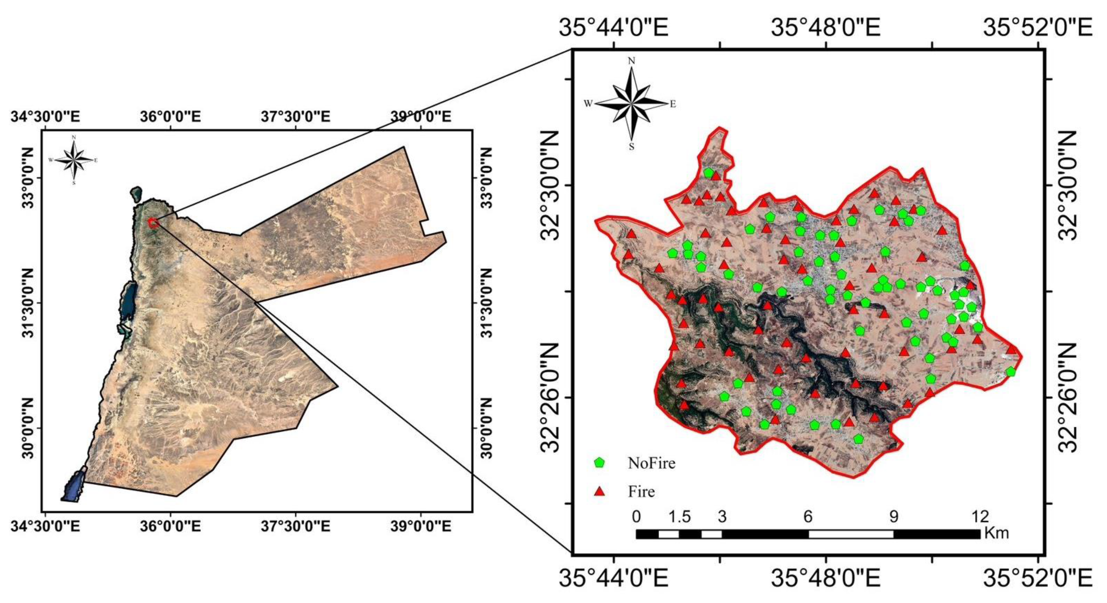
The Northern Mazar District is situated in the northern part of Jordan (
Figure 1). It can be found at the geographical coordinates of 32°28′21″ N and 35°47′34″ E. In terms of local administrative divisions, it falls under the jurisdiction of Irbid Governorate. The governorate is composed of nine administrative districts, namely Irbid city, Al Hisn, Al Mazar al Shamali, Ar Ramtha, Sama al-Rousan, Der Abi Saeed, North Shuneh, Taybeh, and Kufr Asad. The Southern District of the Irbid Governorate is the Northern Mazar District. Its total area is 63.7 km
2, accounting for around 4% of the entire Irbid Governorate, which has an area of 1571.8 km
2. The Northern Mazar District comprises nine villages which differ in size and population. These villages include Al-Mazar Al-Shamali, Enaba, Deir Yusef, Arhaba, Zobia, Jahfah, Samad, Zaatara, Habka, and Hofa.
Based on the data of the Department of Statistics, Jordan, Irbid Governorate had a population of 2,050,300 individuals in 2021. During that year, the Northern Mazar District accounted for 90,840 people, comprising 18,254 families, which represents approximately 4.43% of Irbid Governorate’s total population. Considering these figures, the Northern Mazar District ranks as the seventh most populous district within the governorate of Irbid.
The Northern Mazar District is characterized by its mountainous terrain, which is an extension of the topography found in the adjacent Ajloun Governorate to the south. The primary occupation and source of income for the residents of this district is agriculture. There is widespread cultivation of various fruit-bearing trees such as almonds, olives, and grapes. Additionally, parts of the southern region of the Northern Mazar District are covered by natural forests consisting mainly of oak and pine trees, which extend from the Ajloun Governorate to the north. To safeguard the natural habitats in this district, the Jordanian government has taken action by designating a portion of it as the Barqash Nature Reserve. Livestock raising is another significant activity in this district, taking advantage of the fertile agricultural lands available. Livestock raising practices within the district vary, ranging from individual endeavors to organized, large-scale farms that employ modern methods.
The study area exhibits a pleasant and attractive climate for tourism, characterized by mild summers with an average temperature of approximately 25 °C. However, winters in this district are cold, and temperatures frequently drop below 0 °C during this season. Snowfall is also common in certain parts of the Northern Mazar District during winter. In terms of precipitation, the annual rainfall in this district ranges from 400 to 600 mm, making it one of the areas in Jordan with the highest rainfall rates. As a result, the study area boasts a remarkable richness of biodiversity. However, the presence of dry weeds and field crops during the summer and autumn months increases the risk of forest fires in this region.
2.1. Preparation of Inventory Map
To create the forest fire inventory map, information was gathered from the General Directorate of Civil Defense in the Northern Mazar District regarding seventy locations within the study area that experienced forest fires between 1991 and 2021. The Civil Defense Directorate in the Northern Mazar District has generated these samples by analyzing the polygons that have been affected by fire using the “Create Random Points” technique in the GIS environment. Additionally, another set of seventy locations within the study area, which had no history of forest fires, were identified to develop data-driven models. Among these locations, seventy percent (98 locations) were utilized for constructing the data-driven models, while the remaining thirty percent (42 locations) were reserved for validating the developed models. These samples were selected based on random sampling for creating the training and test datasets. The validation dataset was also utilized to verify the accuracy of the knowledge-based models.
2.2. Factors Contributing to Forest Fires
Following consultations with experts and a thorough review of the relevant literature, twelve factors were selected for the FFS mapping. These factors were chosen based on data availability and their significance in assessing fire spread. Subsequently, the reported values of each factor within the study area were classified into relevant subcategories. A detailed overview of each factor will be provided.
2.2.1. Elevation
The elevation of an area plays a crucial role in determining various climatic conditions, including temperature, humidity, the presence of dry organic materials, as well as the intensity and direction of winds. All of these factors contribute significantly to the risks of ignition and fire spread [
3].
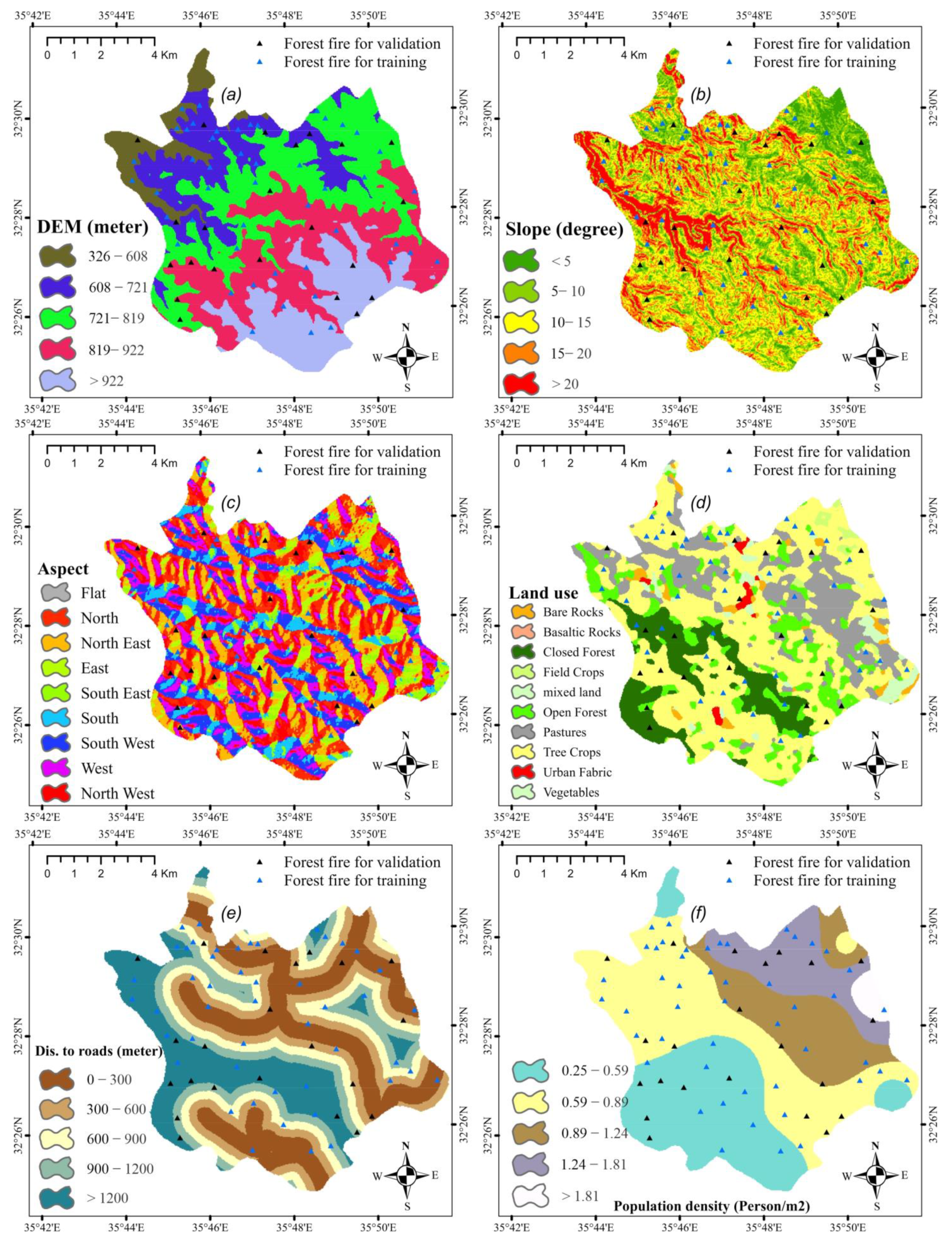
Figure 2a depicts an elevation map specifically for the study district, highlighting variations in elevation ranging from 326 to 1096 m above mean sea level (msl).
2.2.2. Slope
The slope of the land significantly influences the direction and speed at which a fire spreads [
24]. Typically, fires tend to propagate in an up-slope direction, and their rate of spread increases in such conditions due to enhanced connectivity, preheating, and ignition along the uphill path [
1].
Figure 2b illustrates the slope map specifically for the study area, indicating that slopes within the district varied from flat lands (0 degrees) to steeper slopes of up to 55.72 degrees.
2.2.3. Aspect
Aspect refers to how sunlight, temperature, and humidity impact the Earth’s surface [
24]. An aspect map provides details about the slope and orientation of a specific area terrain. These maps are valuable for assessing landscape features and the quantity of sunlight that a location receives, which in turn affects its temperature [
25], and, consequently, its temperature. In
Figure 2c, it can be observed that the aspect values in the study region varied from −1 (representing flat areas) to 359.356.
2.2.4. Land Use
In this study, the land cover and land use attributes of the study area have been classified into eight categories (
Figure 2d).
2.2.5. Distance to Roads
The closeness of forests to roads enhances their vulnerability to fires due to various human-induced disturbances in the forest ecosystem [
1]. As shown in
Figure 2e, the study area exhibited distances to roads ranging from 0 m to over 1200 m.
2.2.6. Population Density
An increased concentration of people living near forests indicates a greater reliance on forest resources, which can result in an elevated risk of forest fire incidents due to human activities within the forests [
26].
Figure 2f reveals that population density in the study area ranged from 0.25 to 2.58 individuals per square kilometer.
2.2.7. Wind Speed
High wind speeds enhance the presence of fresh oxygen in the atmosphere, which can potentially contribute to the spread of fires [
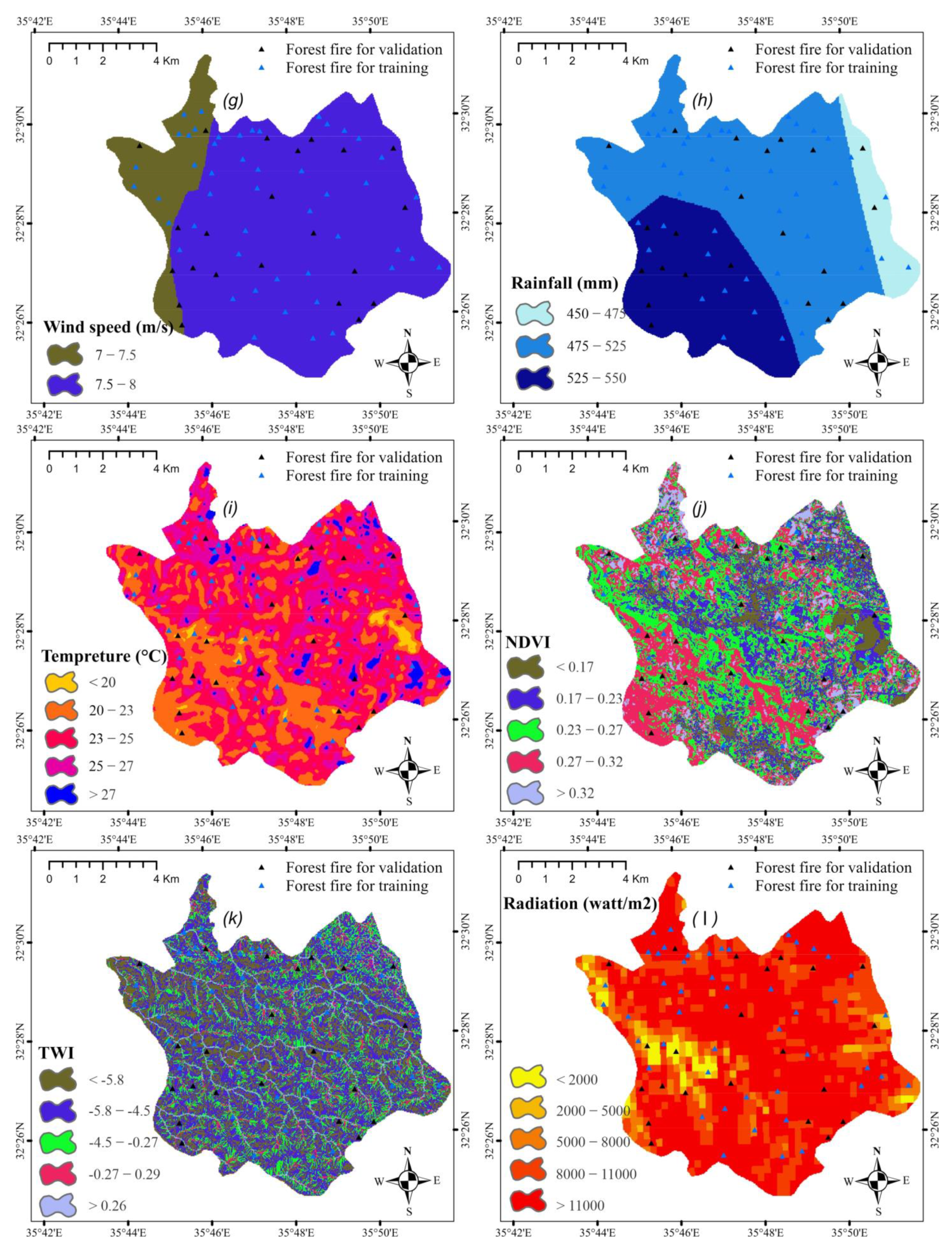
25]. Within the study area, the investigation revealed that wind speeds varied between 7 and 8 m per second, as depicted in
Figure 2g.
2.2.8. Rainfall
Rainfall plays a vital role in regulating humidity and maintaining the water balance [
24] and is inversely related to forest fires [
25]. In the study area, the average annual rainfall depths varied from 450 mm to 550 mm, as illustrated in
Figure 2h.
2.2.9. Temperature
The likelihood of a fire spread increases when there is a combination of high temperature and low humidity [
24]. Forest fires have a direct relationship with this combination of weather conditions [
25]. According to
Figure 2i, the temperature in the study area ranges from 16.47 to 30.04 °C.
2.2.10. NDVI
Normalized difference vegetation index (NDVI) is a widely used indicator for the presence and condition of green vegetation. High NDVI values indicate healthier vegetation, while low values suggest a lack of vegetation. The NDVI value is calculated by dividing the difference between the near-infrared and red bands of radiation by their sum, resulting in a value between −1 and +1. It is calculated using Equation (1) [
25]:
In the study area, the NDVI values ranged from 0.05 to 0.49 (
Figure 2j).
2.2.11. Topographic Wetness Index (TWI)
The Topographic Wetness Index (TWI) quantifies the influence of land topography on hydrological processes [
27]. It is determined by considering the slope and the size of the contributing area located upstream (Equation (2)):
CA refers to the catchment area on an upward slope, while
Slope represents the steepest slope outward for each grid cell [
25].
Figure 2k illustrates that within the study area, TWI values varied from −8.12 to 9.28.
2.2.12. Solar Radiation
Solar radiation has a notable impact on forest fire occurrences since it serves as the predominant energy source that initiates and spreads fires within forest ecosystems [
28]. According to
Figure 2m, the solar radiation intensity within the study area ranges from 48.56 to 13,075.8 Watts/m
2.
Table 1 shows the source of the factors and their minimum and maximum values.
3. Methodology
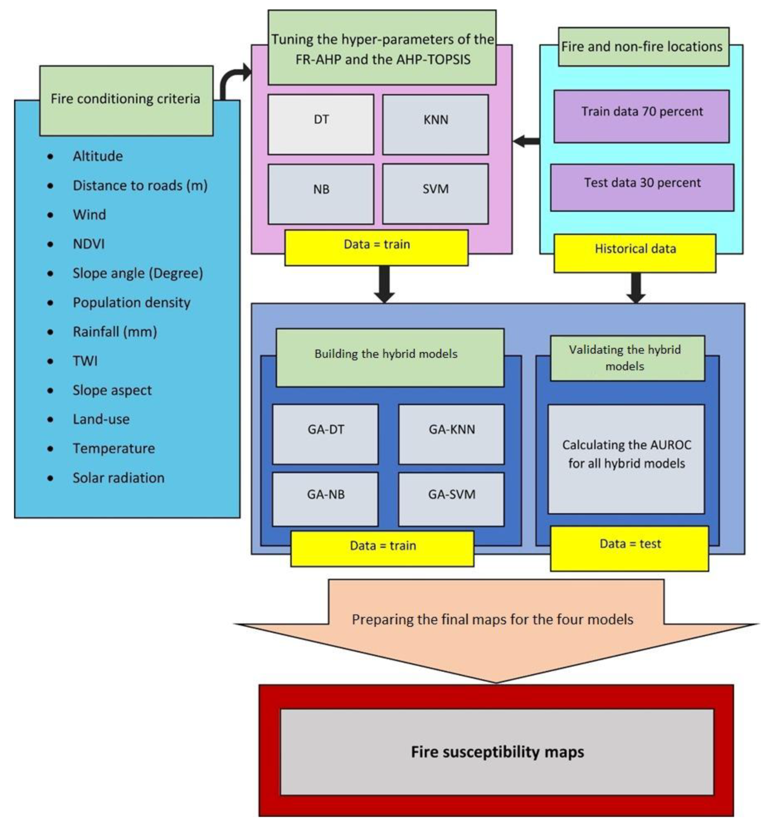
This study conducts a comparison between two knowledge-based models, namely AHP and AHP-TOPSIS, and two newly developed GA-based ensemble data-driven models, boosting and random subspace, in the context of FFS mapping. This study identifies significant factors and prepares separate training and validation datasets consisting of fire and nonfire locations (98 for training and 42 for validation). The ensemble models are utilized to build data-driven models using the training dataset, and the validation dataset is employed to evaluate and validate these models (
Figure 3). These models were built using a dataset consisting of seventy locations with forest fire history and seventy locations without any recorded forest fires. The data were divided into training and validation sets, with 70% (98 locations) allocated to training and the remaining 30% (42 locations) assigned to validation. The averaging method was utilized to generate the final output of the GA-based boosting and GA-based random subspace models. The frequency ratio (FR) method was utilized to assess and assign weights to each class of the factors prior to the modeling process. Subsequently, the AHP was employed to determine the weight of each factor. Finally, the AHP-FR model was developed based on the calculated weights. In fact, at first, the factors that influence the fire incident were classified into subclasses based on previous studies and their ranges of values. Then, FR technique was utilized to rate each subclass of these factors, where high FR scores in each subclass mean more fire incidents with respect to its coverage area. Afterward, the AHP method was applied to calculate the importance of each factor. Experts’ opinions were used to determine the relative superiority of each factor over other factors. They assigned a relative importance score to each pair of factors, based on a scale ranging from 1 to 9. Finally, the weighted overlap approach was employed to combine the outcomes. The weights obtained through the AHP analysis were also used in the modeling process, where the TOPSIS method was utilized.
For the construction of ensemble models in FFS modeling, a GA-based wrapper approach and four algorithms (NB, SVM, kNN, and DT) were utilized to identify the optimal features. These selected features were used in four ML models. Concurrently, ensemble models were developed using boosting and random subspace approaches. Subsequently, the models were validated, and forest fire susceptibility maps were generated (
Figure 3). Detailed information on the models and the evaluation criteria for their performance will be provided in subsequent sections.
3.1. Frequency Ratio (FR)
The Frequency Ratio (FR) was used to determine the correlations between the forest fire locations and each of the aforementioned determinant factors. Through this method, all classes of factors were weighed. The FR is computed by dividing the ratio of the number of fires in each class
i of factor
j (
) by the total number of fires (
F) and then dividing it by the ratio of the area of class
to the overall area (
A) of the study area according to Equation (3) [
29]:
The FR values obtained were standardized and normalized using Equation (4) [
30]:
where
is the normalized
FR values,
is the
FR of the
th subclass of factor
and
is the sum of the
FR values of factor
.
In addition, the prediction rate (PR) is used to evaluate the overall impact of the factors within the FR model. It is calculated according to Equation (5) [
30]:
3.2. Analytic Hierarchy Process (AHP)
The Analytic Hierarchy Process (AHP) is a widely recognized method in multicriteria decision-making (MCDM) [
31]. In the AHP, different criteria are assigned weights based on a specific objective, aiming to identify the most optimal choice [
31]. This technique involves three primary steps [
32]:
The initial step involves defining the objective, criteria, and available alternatives for a given problem. In this particular study, the objective focused on FFS, while the criteria consisted of 12 factors that determine forest fire occurrence. These factors were identified and specified by the experts involved in this study.
- 2.
Making pairwise comparisons and weighting
During this step, the criteria are arranged in a matrix called the pairwise comparison matrix. This matrix allows for the comparison and weighting of each criterion by considering them two by two. The pairwise comparison is performed by assigning importance weights to the elements within each cell of the matrix. Typically, a scale of 1–9 is used to assess the relative importance of each factor being evaluated. A value of 9 signifies high importance, while a value of 1 indicates equal importance and preference (refer to
Table 2). Importantly, the pairwise comparison matrix is an invertible matrix, meaning that if the comparative value of the importance of a row element ‘a’ to a column element ‘b’ is 9, then the comparative value of the importance of the column element ‘b’ to the row element ‘a’ would be 1/9.
- 3.
Calculating the consistency rate
In the AHP, the consistency rate (CR) is a metric that assesses the coherence of pairwise comparisons. It quantifies the accuracy and correctness of the valuations made in these comparisons. The CR is calculated using Equation (6) (Saaty, 1987):
where
RI is the random index selected from
Table 3 based on the number of criteria (
n), and
CI is the consistency index. It is calculated using Equation (7) [
32]:
where
is the largest eigenvalue of the comparison matrix.
If the CR is equal to or less than 0.1, it indicates that the valuations and compari-sons are reliable and accurate. However, if the CR exceeds 0.1, it signifies a need for modifications to the valuations and comparisons.
3.3. TOPSIS
TOPSIS is a MCDM technique that was created by Hwang and Yoon in 1981. This model operates under the assumption that the optimal solution is characterized by having the shortest Euclidean distance from the positive ideal solution and the longest distance from the negative ideal solution [
33]. The positive ideal solution aims to maximize the positive features (benefits) and minimize the negative features (costs), while the negative ideal solution seeks to maximize the negative features (costs) and minimize the positive features (benefits).
MCDM problems involve comparing and evaluating different information under specific conditions in order to obtain a suitable ranking. To accomplish this objective, a matrix
is constructed using alternatives
and criteria
. This matrix facilitates the ranking of alternatives and enables the evaluation and comparison of different criteria. The TOPSIS algorithm is then implemented by following the subsequent steps [
33,
34]:
Creating the decision matrix based on m criteria and n alternatives.
Calculating the normalized decision matrix r
ij using Equation (8):
where
is the numerical value obtained from the intersection of alternatives and criteria.
Calculating the weighted normalized decision matrix (w
ij) based on the weighted normalized value of v
ij by multiplying the normalized decision matrix by the weight (
) allocated to every criterion according to Equation (9):
Determining the positive ideal solution and the negative ideal solution by using Equations (10) and (11):
In these equations, J pertains to benefit criteria, whereas J’ is related to cost criteria.
Calculating the separation values by using the n-dimensional Euclidean distances:
The distance between every alternative from a positive ideal solution (s
+j) is calculated by Equation (12):
Similarly, distance of each alternative from a negative ideal solution (
s−j) is calculated as follows:
Calculating the relative proximity to an ideal solution, which can be obtained from Equation (14):
Ranking the alternatives based on their relative proximity values.
In this regard, the alternative that has the highest value is considered the best alternative.
The present study utilized the AHP method to assign weights to criteria within the TOPSIS model.
3.4. Genetic Algorithm-Based Ensemble Models
Sagi and Rokach (2018) provided a definition of ensemble learning as the practice of generating and merging multiple inducers to address specific machine learning tasks. Dong et al. (2020) stated that ensemble learning strives to seamlessly integrate diverse machine learning algorithms into a unified framework. This enables effective utilization of the complementary information from each integrated algorithm, resulting in improved performance for the overall model.
Ensemble models are becoming more prevalent in different fields and research studies. In this particular study, GA-based boosting and random subspace methods were employed for the FFS mapping. Prior to constructing the ensemble models, feature selection was conducted using the wrapper approach with GA and four classifiers: SVM, DT, NB, and kNN. Once the optimal features were determined by the GA-SVM, GA-DT, GA-NB, and GA-kNN models, these features were utilized to create ensemble models using the boosting and random subspace approaches, utilizing four machine learning models.
The boosting approach involves initially constructing a model using a training dataset. Then, the samples that were incorrectly classified by the initial model are identified and presented to the next model for further learning. This process is repeated iteratively to build the final ensemble model. On the other hand, in the random subspace approach, the models are created by randomly selecting features to build the ensemble model. In this study, the four commonly used and well-known classifiers, NB, SVM, kNN, and DT, were used for this purpose.
The NB algorithm is a straightforward classifier that relies on the Bayes’ theorem [
35,
36,
37]. In the NB classification, it assumes that features are independent and aims to determine posterior probabilities. The DT algorithm utilizes a flowchart-like structure where samples are classified by traversing from the root node to the leaf nodes [
38]. The kNN algorithm is a classification technique that determines the class for a new sample by analyzing a specified number of most similar neighbors or samples [
39]. This method requires a distance criterion, such as the Euclidean distance, to measure similarity between samples. The SVM algorithm seeks to identify the optimal hyperplane that can separate data from two classes with the maximum margin [
24].
3.5. Model Accuracy Assessment
In this study, the accuracy of the models was assessed using the area under the receiver operating characteristic curve (AUROCC). The
y-axis and
x-axis values of this curve were obtained using Equations (15) and (16) [
40,
41]:
where
TP represents correctly predicted positive samples (occurrence);
TN represents correctly predicted negative samples (nonoccurrence); FP represents negative samples incorrectly classified as positive; and FN represents positive samples incorrectly classified as negative by the model. In this study, the AUROCC values were used to assess the predictive capabilities of the models in distinguishing between locations with forest fire incidence and those without.
4. Results
In
Table 4, the findings regarding the correlation between forest fires and various factors generated by the FR model are summarized. The analysis reveals that the classes of altitude between 326–608 m and 608–721 m exhibit the highest FR values in relation to forest fires. In terms of other factors studied as determinants of forest fires, this study indicates that the highest FR values are associated with a slope ranging from 10–15 degrees, a north-facing aspect, distances to roads between 300 and 600 m, a population density of 1.24–1.81 person/km
2, land use for field crops, wind speeds of 7–7.5 m/s, rainfall depths of 475–525 mm, temperatures exceeding 27 °C, NDVI values greater than 0.32, TWI values between −2.7 and 0.26, and solar radiation intensities below 2000 watt/m
2.
Following the computation of PR values for each factor, these values were used in creating the AHP pairwise comparison matrix, as represented in
Table 5 for the FR-AHP model. To illustrate, the PR value for the altitude factor is 1.93, while the PR value for the slope factor is 1.60. By dividing 1.93 by 1.60, we determine that the relative importance of altitude compared to slope is 1.20.
To determine the weights in the AHP, it is necessary to normalize the pairwise comparison matrix (
Table 6). Subsequently, the weights were calculated using arithmetic means. The AHP results indicated that the factors of land use and NDVI had the highest weights, specifically 0.22 and 0.13, respectively. Conversely, solar radiation and slope had the lowest weight, both at 0.05 (as shown in
Table 6). To generate the FFS map using the FR-AHP model within the GIS environment, each subclass of the factors (
Table 4) was assigned FR values. The criteria weights obtained through the FR-AHP method (
Table 6) were utilized in a weighted overlay analysis. This process resulted in the production of the FFS map.
In the AHP-TOPSIS model, the initial step involved establishing the PWCM of AHP. This matrix is represented in
Table 7. The values in the matrix were then normalized to obtain the final weights. Additionally, the preferences of the decision maker were taken into account using a scale ranging from 1 to 9. The AHP model demonstrated a low inconsistency rate of 0.03, indicating that the evaluations in the pairwise comparison matrix were consistent. Referring to
Table 7, it can be observed that the land use factor carried the highest weight of 0.257, whereas the TWI had the lowest weight of 0.02.
As shown in
Table 7, the AHP technique was used to determine the weights of 12 factors related to forest fires. These weights were then used in the creation of a TOPSIS model using
MATLAB software. To display the values of the 12 factors and other calculated parameters derived from the AHP-TOPSIS technique, a random sample of 5000 points was selected from a total of 31,654 points (
Table 8). In the subsequent step, the criteria values were rescaled and multiplied by the weights obtained from the AHP method. The primary values of the 12 factors were normalized using Equations (7) and (8). The values of
A+ and
A− were calculated using Equations (9) and (10) (
Table 9). Then, Equations (11) and (12) were employed to determine the separation of each alternative from the positive ideal solution (
) and the negative ideal solution (
), respectively (
Table 10). Following this, Equation (13) was used to compute the relative proximity to an ideal solution (
) and rank the various alternatives (
Table 10). The weights generated by this technique were incorporated into the attribute table of the combined layer of factors. Consequently, FFS maps were created in the GIS environment.
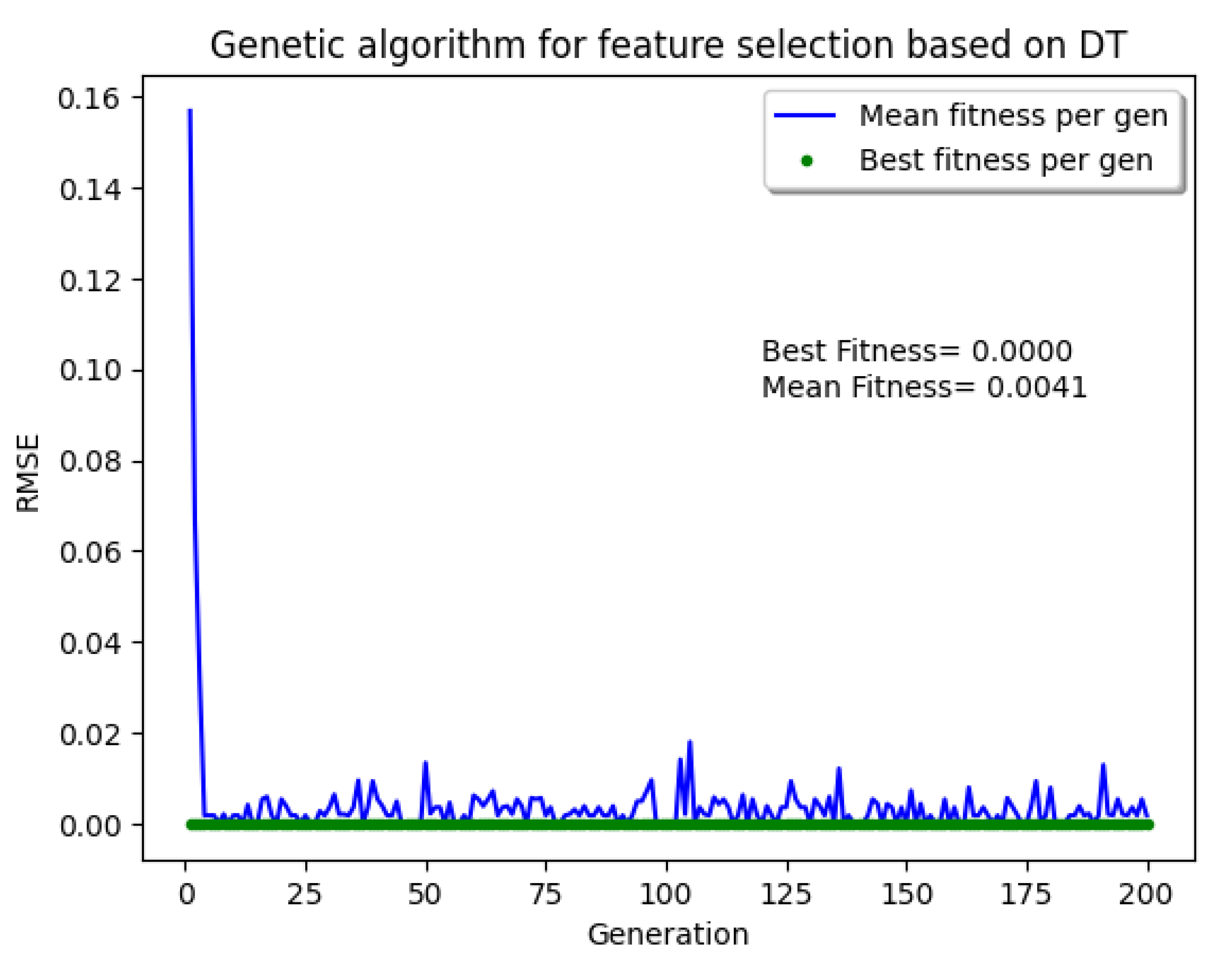
Figure 4 and
Figure 5 depict the mean and best fitness values obtained from the GA-based feature selection applied to identify optimal features using wrapper approaches and four algorithms of DT, kNN, NB, and SVM models. The root mean square error (RMSE) was used as the performance measure in the feature selection process to assess the fitness of each feasible solution. The GA-based feature selection approach employed 200 generations and 20 solutions per generation.
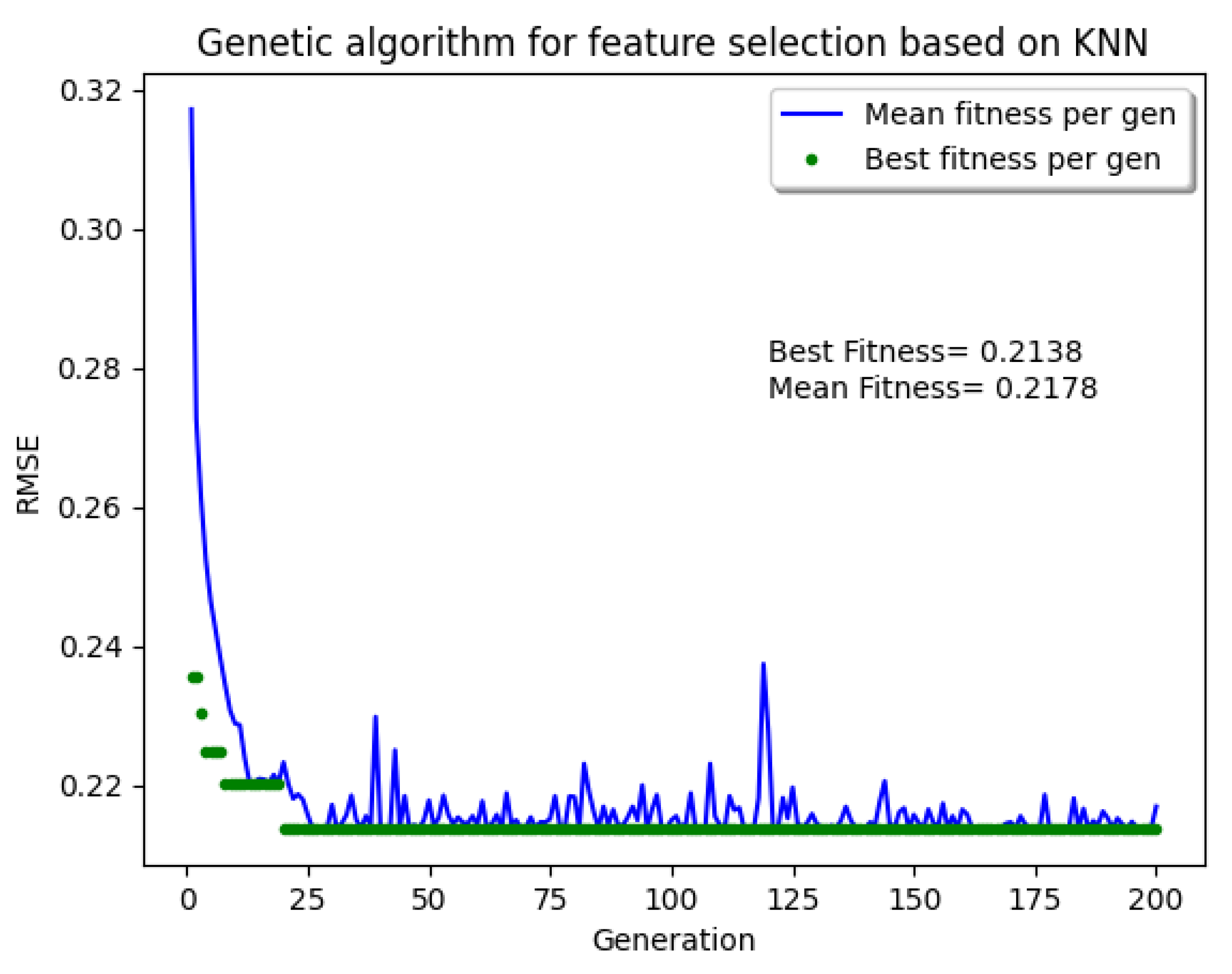
Figure 4 illustrates that the GA-DT model achieved the best fitness value (RMSE = 0), indicating excellent performance. On the other hand, the GA-kNN model reached a stable fitness value after the 21st generation, with an associated RMSE of 0.2178. After completing the feature selection using the GA-DT model, it was determined that the most influential factors for forest fire incidence were land use, distance to roads, NDVI, wind speed, TWI, and temperature. In the case of the GA-
kNN model, the most influential factors were found to be NDVI, aspect, and temperature.
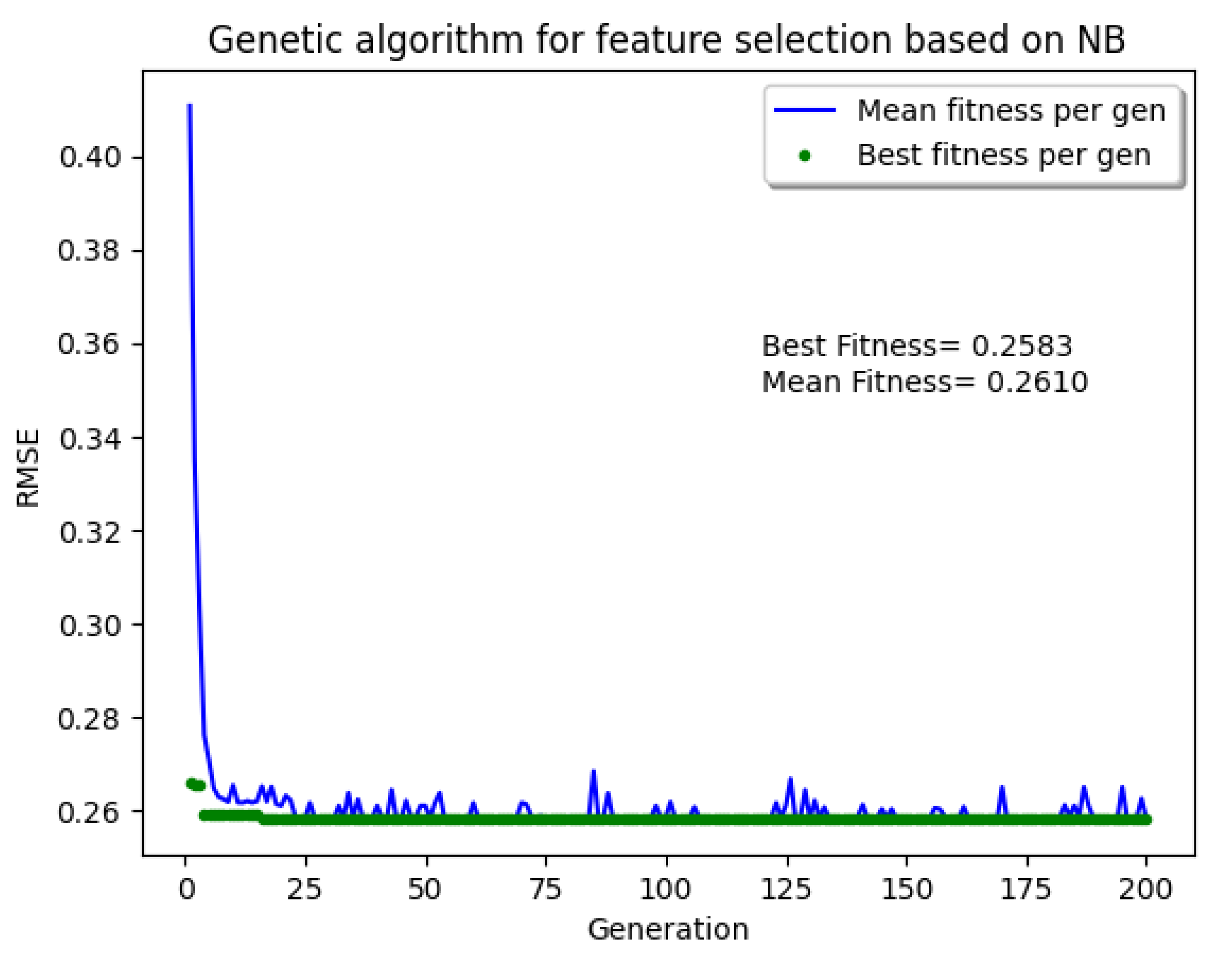
The GA-NB model for feature selection reached an RMSE value of 0.2583 after the 18th generation, as shown in
Figure 6. In this model, population density, solar radiation, rainfall, NDVI, aspect, and temperature were identified as the significant factors for the modeling process.
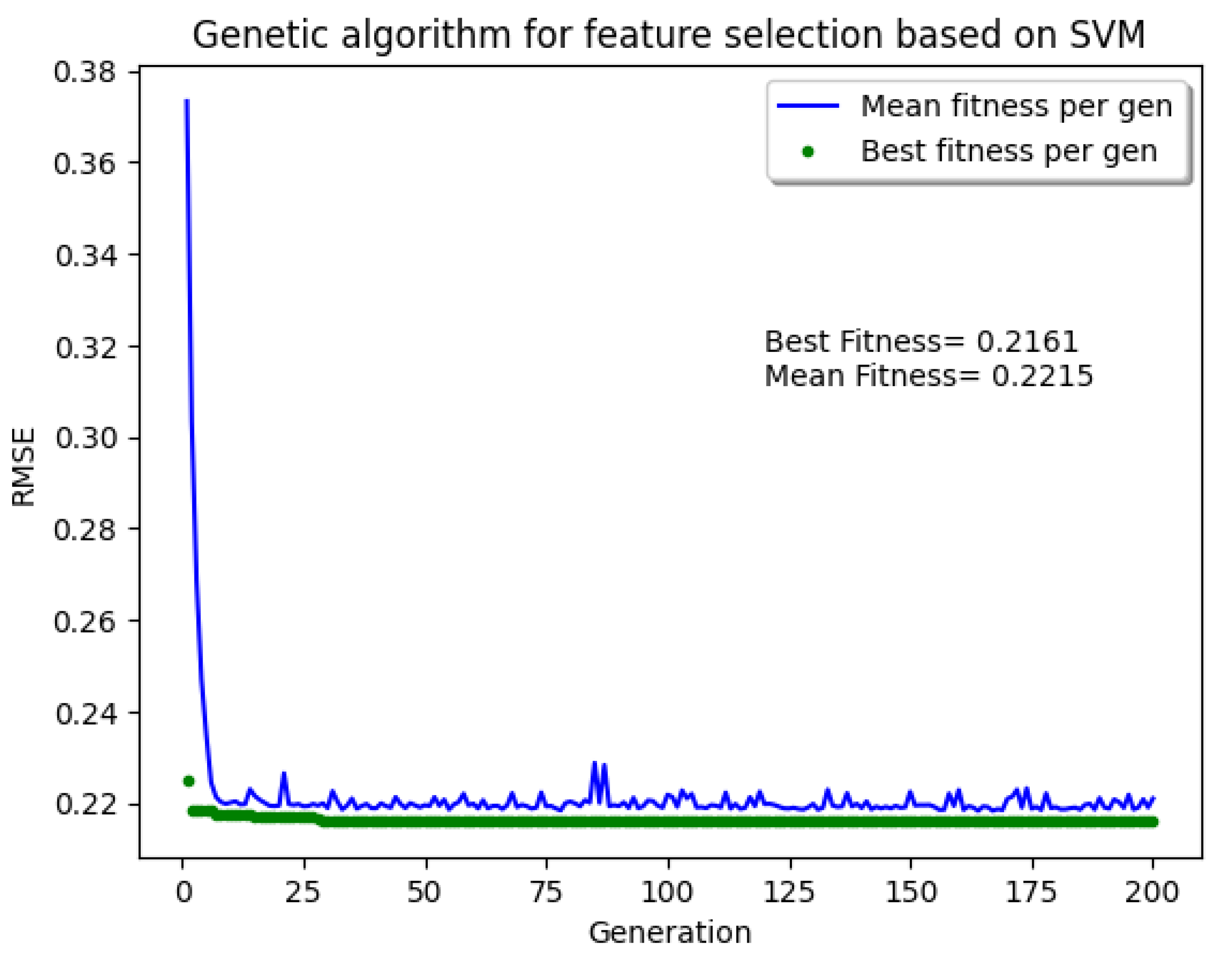
Figure 7 demonstrates that the GA-SVM model reached a stable fitness value after the 28th generation, with the RMSE stabilizing at 0.2215. The findings indicate that population density, distance to roads, solar radiation, NDVI, wind speed, aspect, and temperature were the most significant factors influencing forest fire incidence by GA-SVM.
Once the optimal factors were determined for each model, six data-driven models were employed: DT, NB, kNN, SVM, GA-based boosting, and GA-based random subspace. Within the GA-based bootstrap and GA-based random subspace models, four integrated models were created: GA-DT, GA-SVM, GA-NB, and GA-kNN.
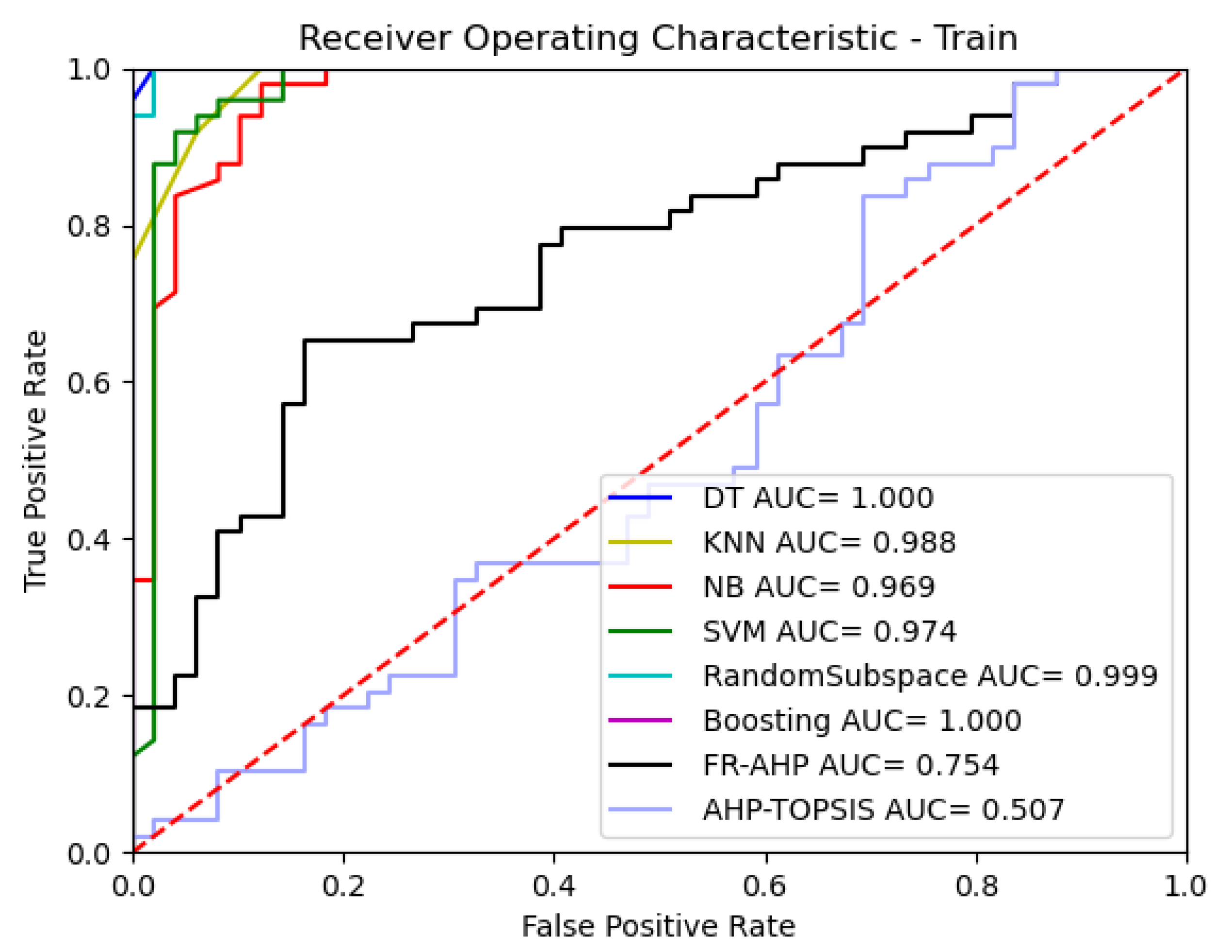
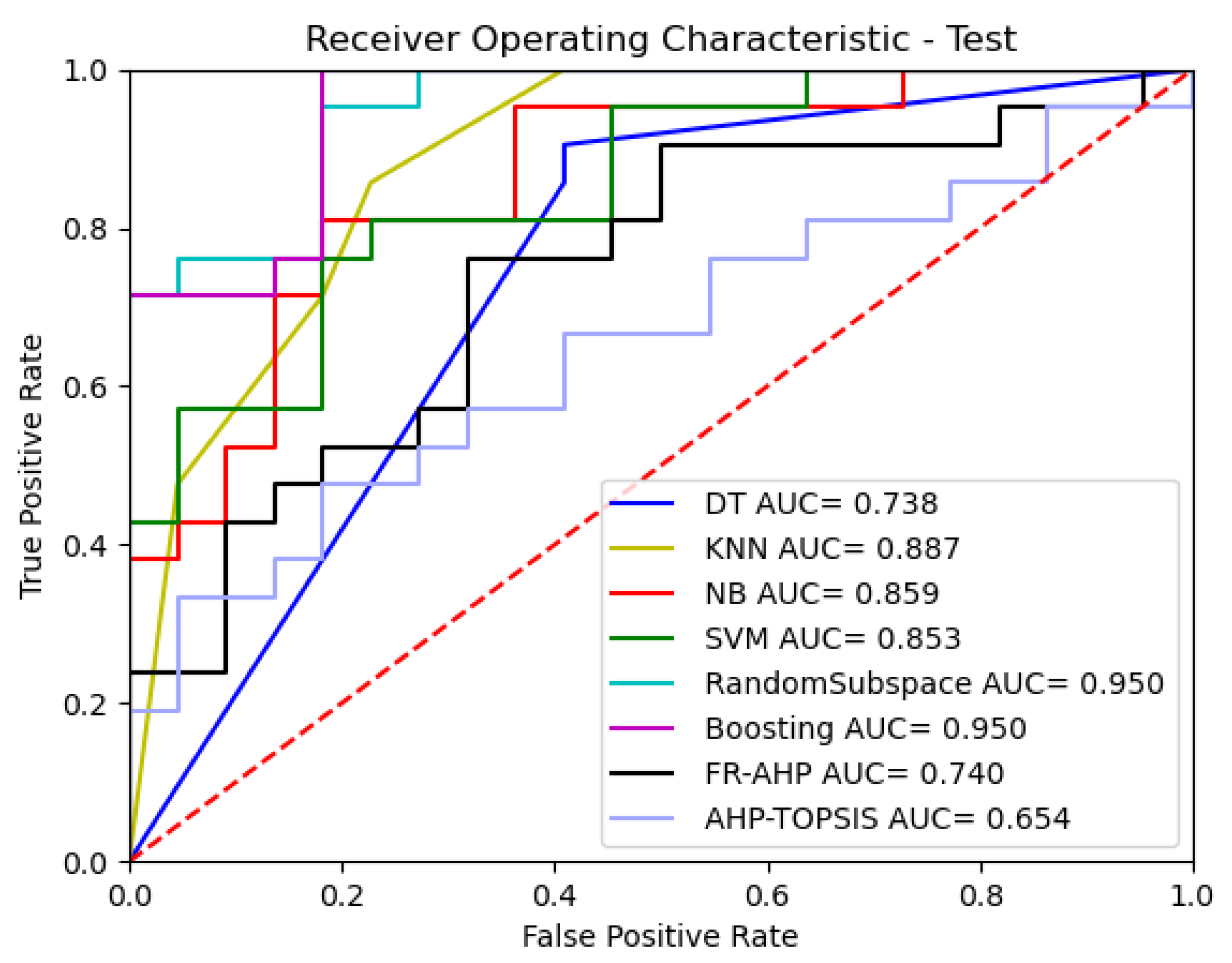
Figure 8 and
Figure 9 show the AUROCCs and the AUC values for the eight models in both the training and testing runs. In both runs, the GA-based ensemble models outperformed the MCDM models in terms of the AUC. In the training runs, the DT and boosting models had the highest AUC values, followed by the random subspace, kNN, SVM, NB, FR-AHP, and AHP-TOPSIS models (
Figure 8). In the testing runs, the boosting and random subspace models exhibited the highest AUC values, while the single models and MCDM techniques displayed lower AUC values (
Figure 9).
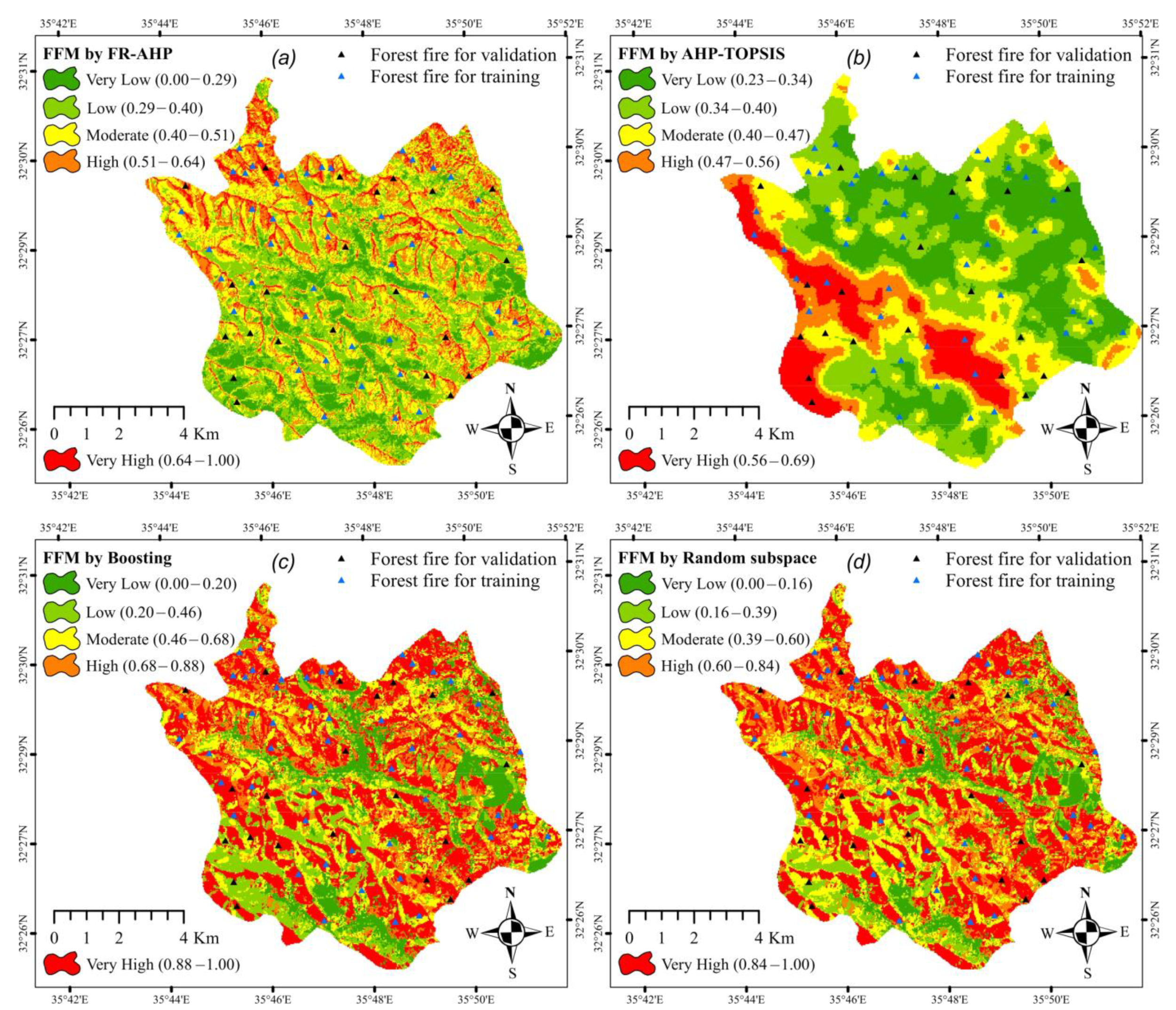
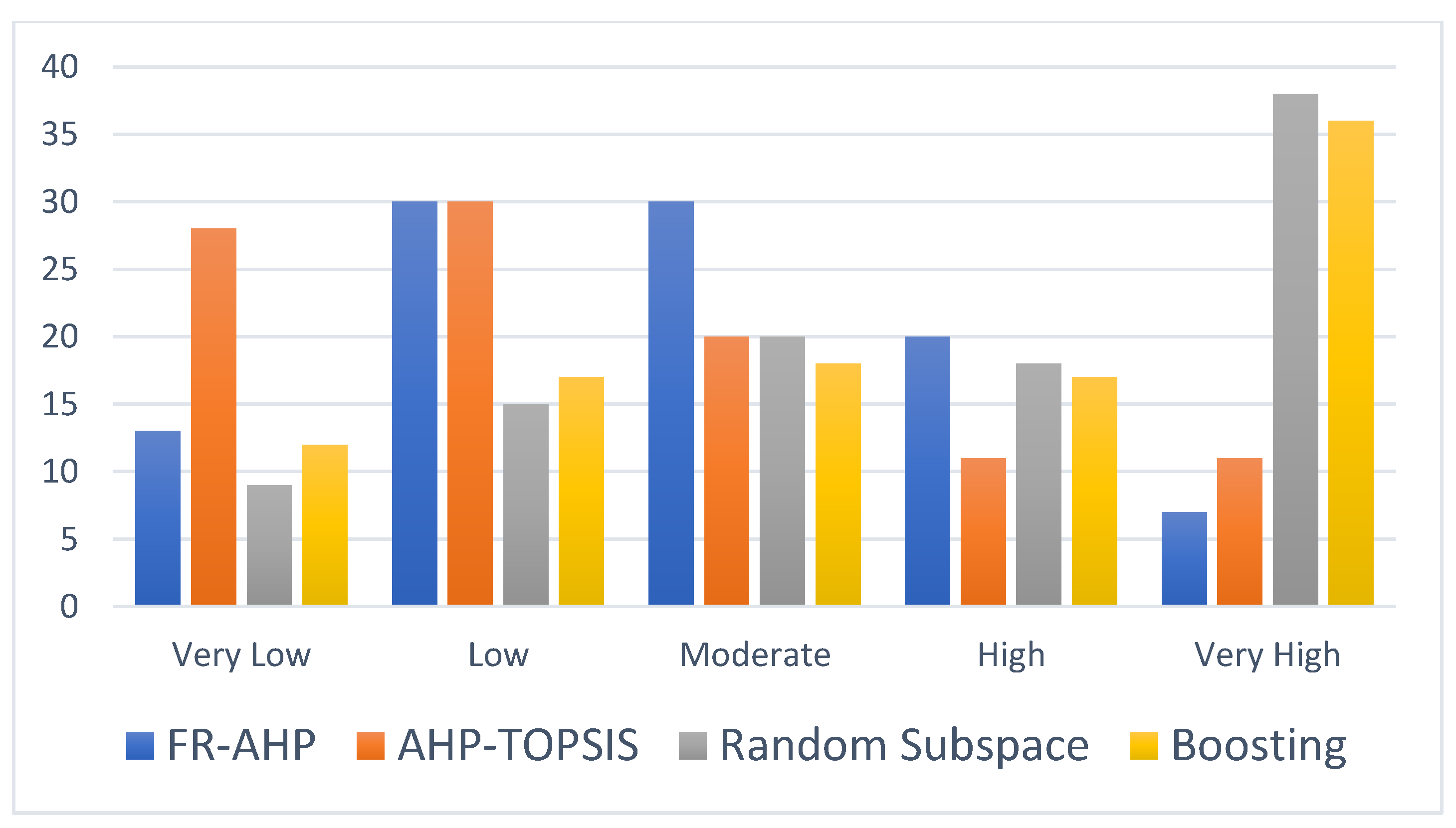
The FFS maps produced by the FR-AHP, AHP-TOPSIS, boosting, and random subspace models are depicted in
Figure 10. The entire area’s fire susceptibility was classified into five classes: very low, low, moderate, high, and very high susceptibilities. It is evident from
Figure 10 that the allocation of areas to each class varies among the different models. Moreover,
Figure 11 shows the percentage of susceptibility classes for four models.
The FFS maps in
Figure 10 were classified into five different probability zones using the natural break raster classification technique in GIS environment. This method takes into account the natural grouping of the data and determines breakpoints based on the differences between comparable groups. The reason for using this classification method is because it is data-specific and allows for the zoning of the fire forest susceptibility maps.
5. Discussion
Forests play a crucial role in sustaining human life and provide various essential benefits such as increased soil infiltrability, enhanced water storage capacity, prevention of soil erosion, purification of polluted air, and serving as habitats for diverse animal and plant species. However, forests face significant destruction worldwide due to frequent fires caused by factors such as global warming, human negligence, and intentional burning for land clearance. The loss of forests has severe consequences for humans, animals, plants, and ecosystem processes and services. It is therefore imperative to prevent forest fires to safeguard these invaluable forest systems, processes, and resources. In the unfortunate event of a fire, immediate measures must be taken to prevent its spread.
Understanding the factors contributing to forest fire occurrence is crucial for the development of fire susceptibility maps. Numerous feature selection methods have been proposed, with wrapper-based feature selection being one of the most important approaches. In this study, four feature selection algorithms, namely GA-DT, GA-kNN, GA-SVM, and GA-NB, were employed to identify the influential factors in the forest fire susceptibility mapping. NDVI and temperature consistently emerged as the most significant factors across all algorithms. Previous studies, including those by Fiorucci et al. (2007), Gonzalez-Alonso et al. (1997), Lasaponara (2005), and Illera et al. (1996), have also utilized NDVI variations to identify fire-prone areas [
25,
42,
43,
44]. Similarly, in our study, NDVI was identified as a critical indicator of fire occurrence, showing a direct correlation between increased NDVI values and the number of fire incidents. However, NDVI can identify areas with potential fuel sources for burning, but it is not an ideal substitute for directly measuring fuel quantity or quality. Temperature was another prominent factor, aligning with research conducted by [
26,
45]. Temperature plays a significant role in fire behavior. Higher temperatures increase the chances of fire ignition and make it more difficult to control fires once they have started.
Identifying forested areas at high risk of fire and implementing preventive measures are essential for effective fire management. In this context, our study compared the FFS mapping capabilities of two knowledge-based models (AHP and AHP-TOPSIS) with two GA-based ensemble data-driven models (boosting and RS). These models were developed using the NB, kNN, DT, and SVM algorithms to predict areas highly susceptible to forest fires in the Northern Mazar District in Jordan. In recent years, both MCDM techniques and data-driven models have been widely employed by researchers for hazard mapping. Some studies, such as those conducted by Zhu et al. (2018) and Arabameri et al. (2018), have reported superior performance of MCDM techniques over data-driven models [
46,
47], while others, such as Chicas et al. (2022) and Nachappa et al. (2020), have found data-driven models to be more effective [
48,
49]. Therefore, to obtain a reliable forest fire susceptibility map, it is crucial to evaluate and compare both approaches. In our study, data-driven models exhibited better performance compared to expert-based models, consistent with findings from Chicas et al. (2022) and Nachappa et al. (2020).
6. Conclusions
This research highlights the importance of employing advanced ML models to accurately map areas in the Northern Mazar District in Jordan that are highly prone to forest fires. To create the FFS models, a total of 140 locations were chosen. These locations included 70 areas that had experienced forest fires in the past and 70 locations with no known instances of forest fires. Fourteen factors were considered during the analysis, which encompassed elevation, slope, aspect, land use, distance to roads, population density, wind speed, rainfall, temperature, NDVI, TWI, and solar radiation. By comparing knowledge-based models such as AHP and AHP-TOPSIS with GA-based ensemble models such as boosting and RS, developed using algorithms such as NB, kNN, DT, and SVM, it was found that the latter performed better than the former. This suggests that using ML algorithms capable of capturing complex relationships between multiple variables is crucial. Additionally, this study concludes that data-driven models are more precise than knowledge-based models for the FFS mapping.
To gain deeper understanding of this study’s findings, it is crucial to grasp the importance of the variables employed in the modeling and FFS mapping. Through the wrapper approach utilized for feature selection, it was discovered that NDVI and temperature played a significant role in determining an area’s vulnerability to forest fires. NDVI serves as a widely used index indicating the density and health of vegetation. Concerning FFS, NDVI is a vital factor because areas with dense vegetation cover are less prone to experiencing forest fires compared to those with sparse vegetation cover. Conversely, temperature is another critical variable as higher temperatures escalate the likelihood of fire ignition and intensify the challenges involved in controlling them once they start.
The produced FFS maps have the potential to assist in the prevention and control of forest fires by recognizing areas at high risk and implementing precautionary measures before fires occur. For example, pre-establishing rescue and relief stations can considerably decrease response times, enabling firefighters to rapidly contain and extinguish fires. Additionally, the installation of water storage tanks containing ample amounts of water in high-risk regions can serve as a firefighting water source. By placing wireless sensors in wooded regions, fires can be detected, and authorities can be alerted promptly, resulting in quicker response times and more efficient firefighting operations.


 ,
, 
