


Modeling Impact of Transportation Infrastructure-Based Accessibility on the Development of Mixed Land Use Using Deep Neural Networks: Evidence from Jiang’an District, City of Wuhan, China

 ,
,  ,
,  , and
, and 
Abstract
:1. Introduction
2. Literature Review
3. Study Data and Methods
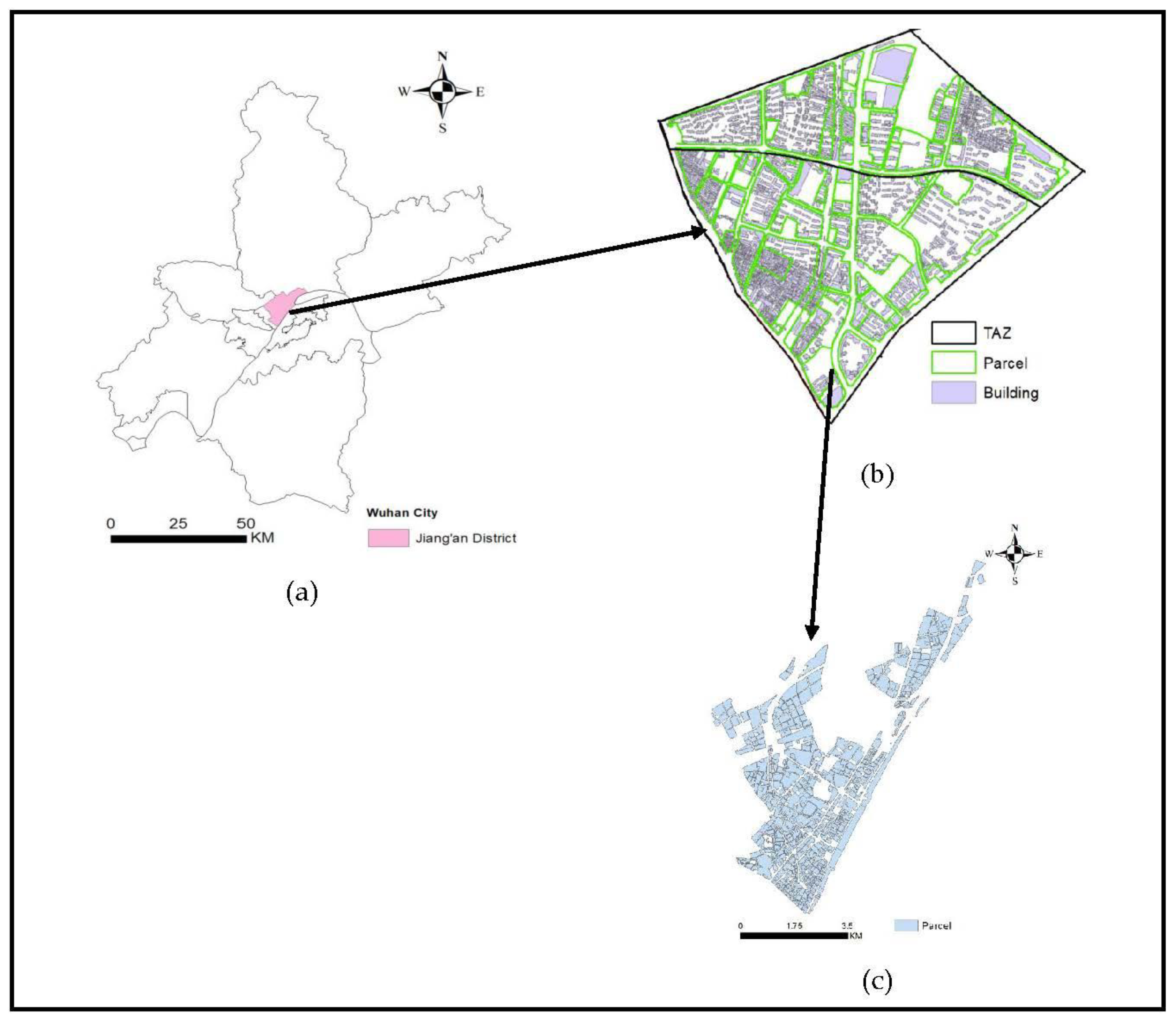
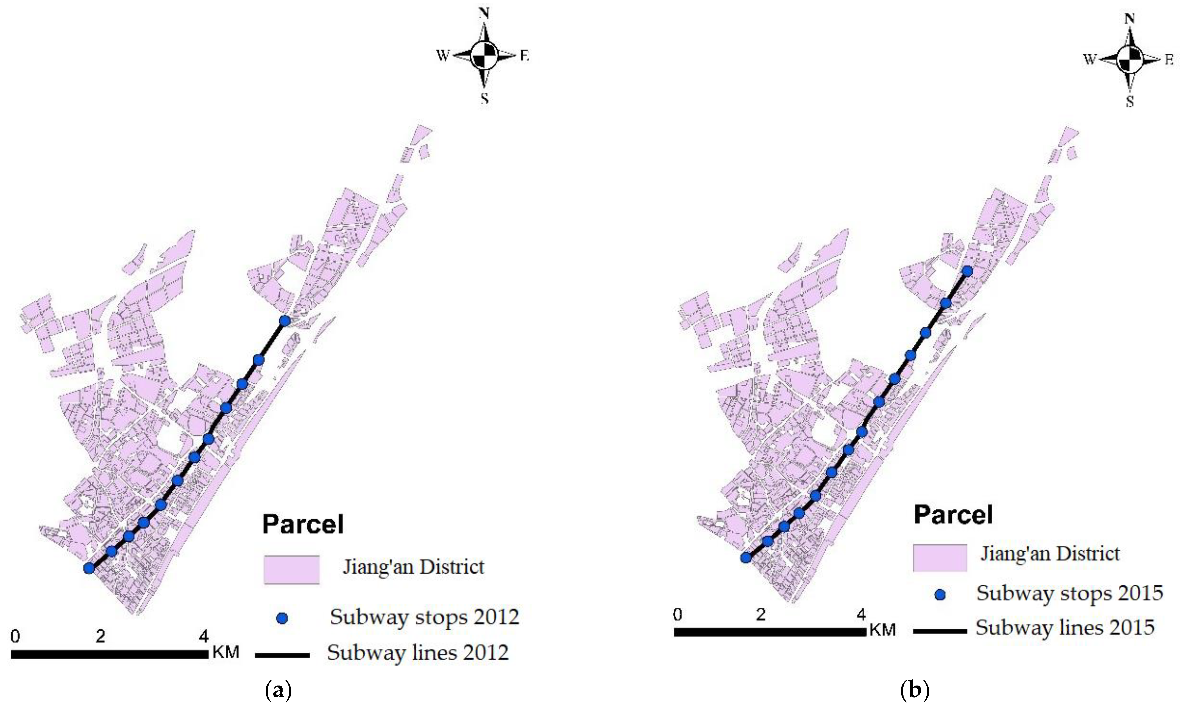
3.1. Dataset
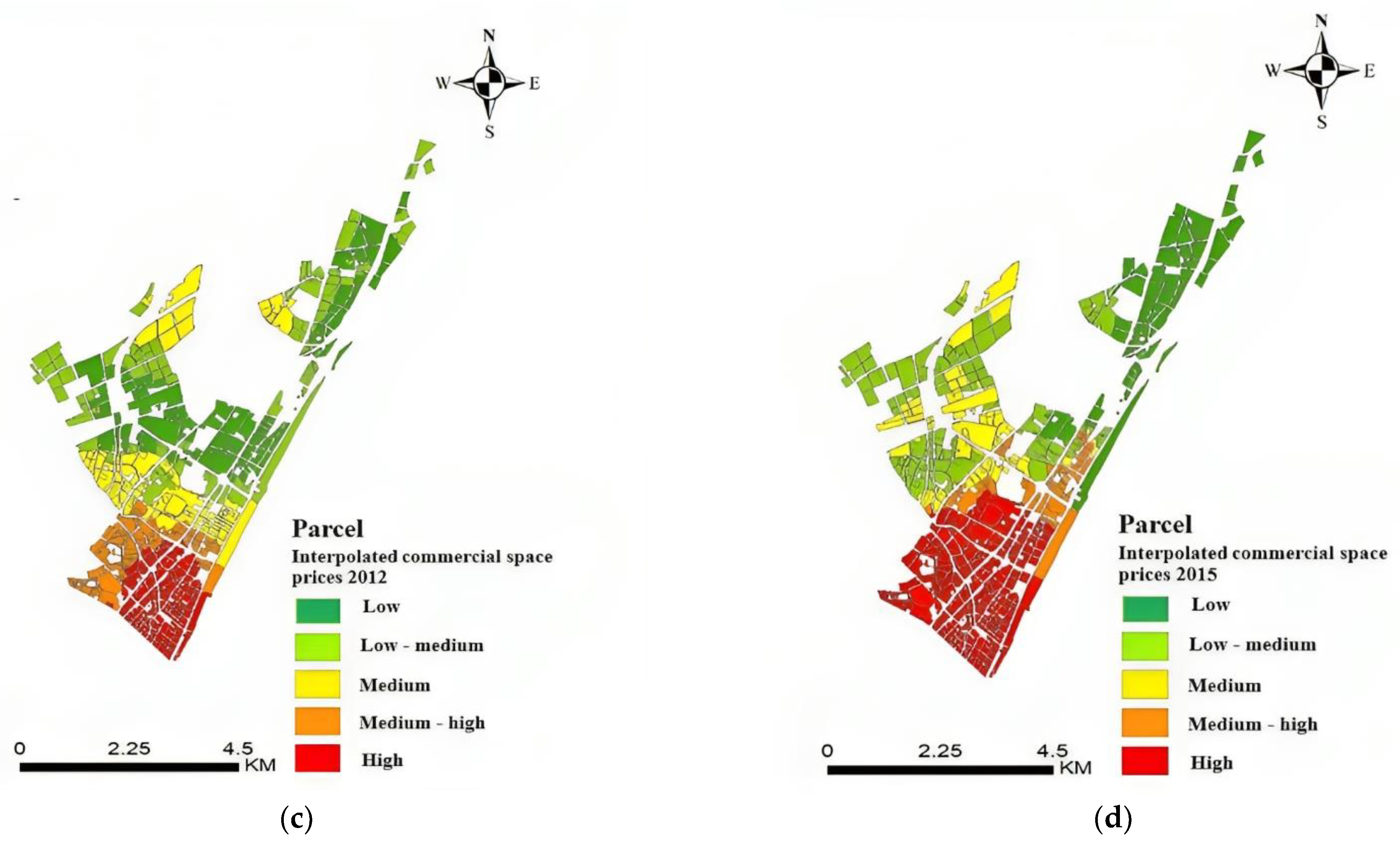
3.2. Floor Space Price Process
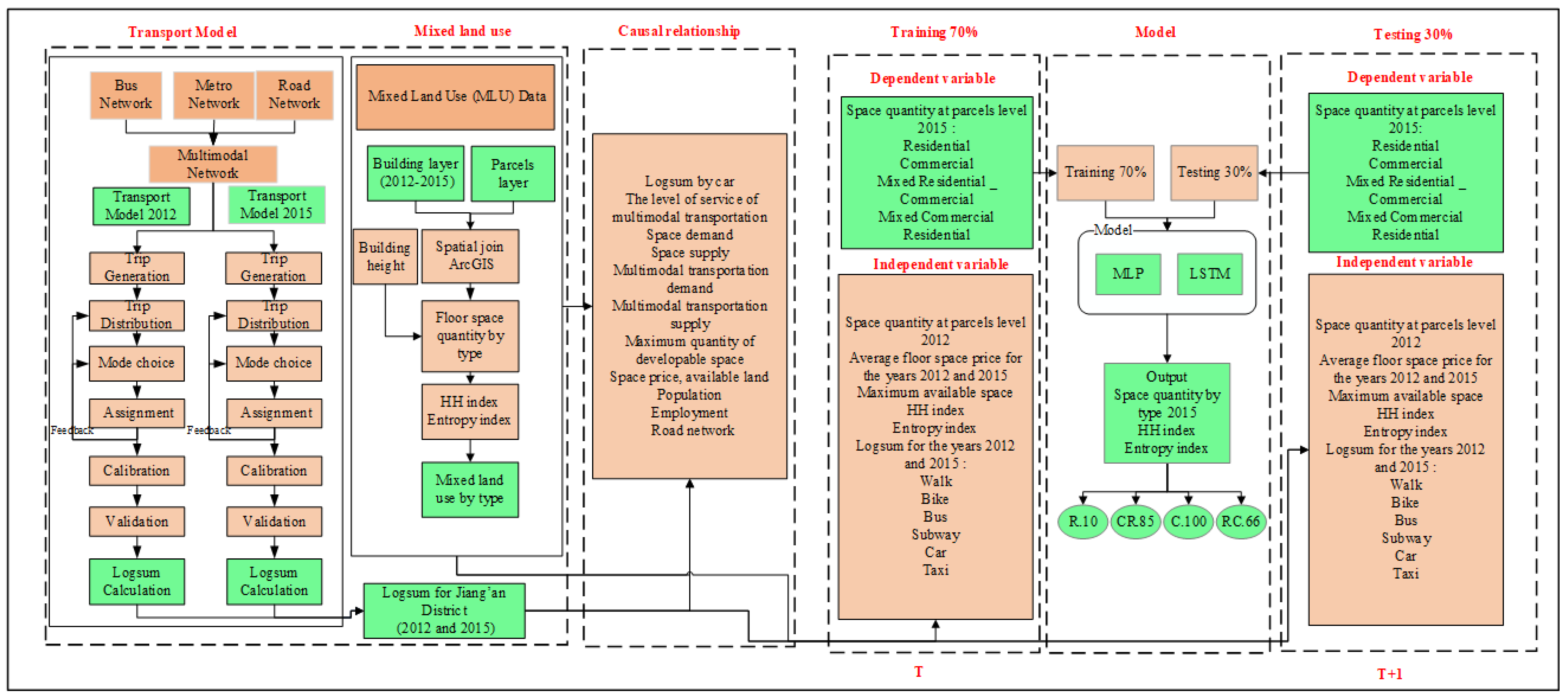
3.3. Methods
- (1)
- Prepare data for models that represent transport supply (subway lines and stops, bus stops and lines, road network), average floor price, and MLU pattern (building and developable land);
- (2)
- The developed multimodal transportation model is used to estimate the logsum by walk, bike, bus, subway, car, and taxi;
- (3)
- The average floor space prices are calculated utilizing the kriging interpolation tool;
- (4)
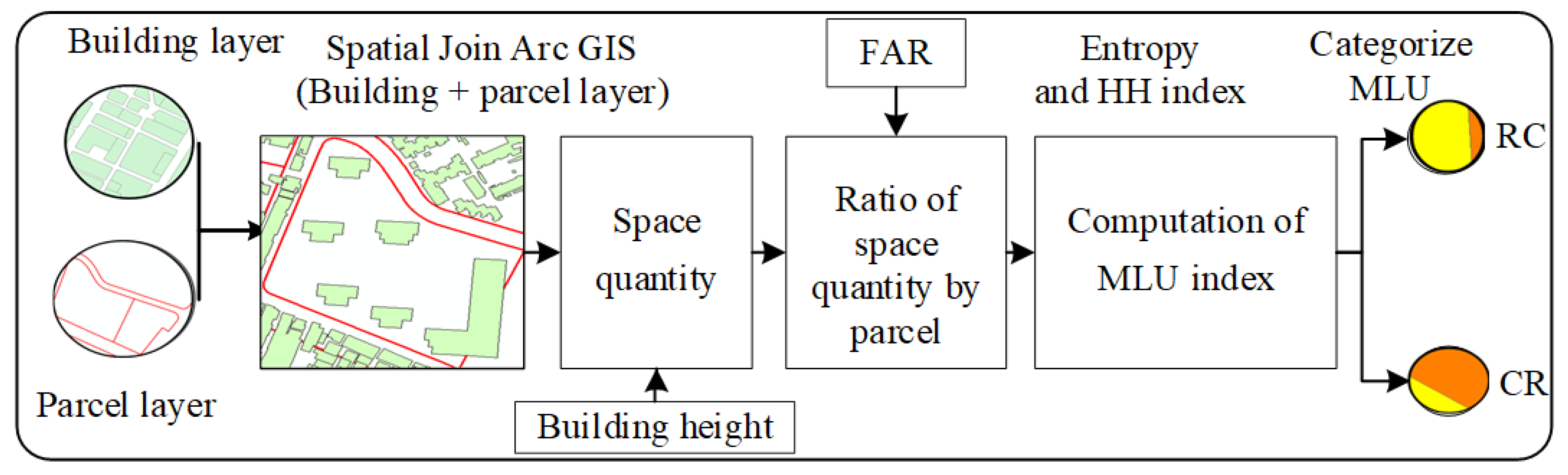
- The spatial join and intersection analysis tool in ArcGIS is utilized to prepare the MLU pattern data at the parcel level. Then, the ENT and HH indexes are employed to represent the degree of MLU;
- (5)
- Utilize the system dynamic framework to examine the causal relationship between transport supply, various other related factors, and MLU;
- (6)
- DNNs (MLP and LSTM) are utilized to forecast the influence of transport supply on MLU;
- (7)
- Finally, compare the accuracy of the LSTM and MLP.
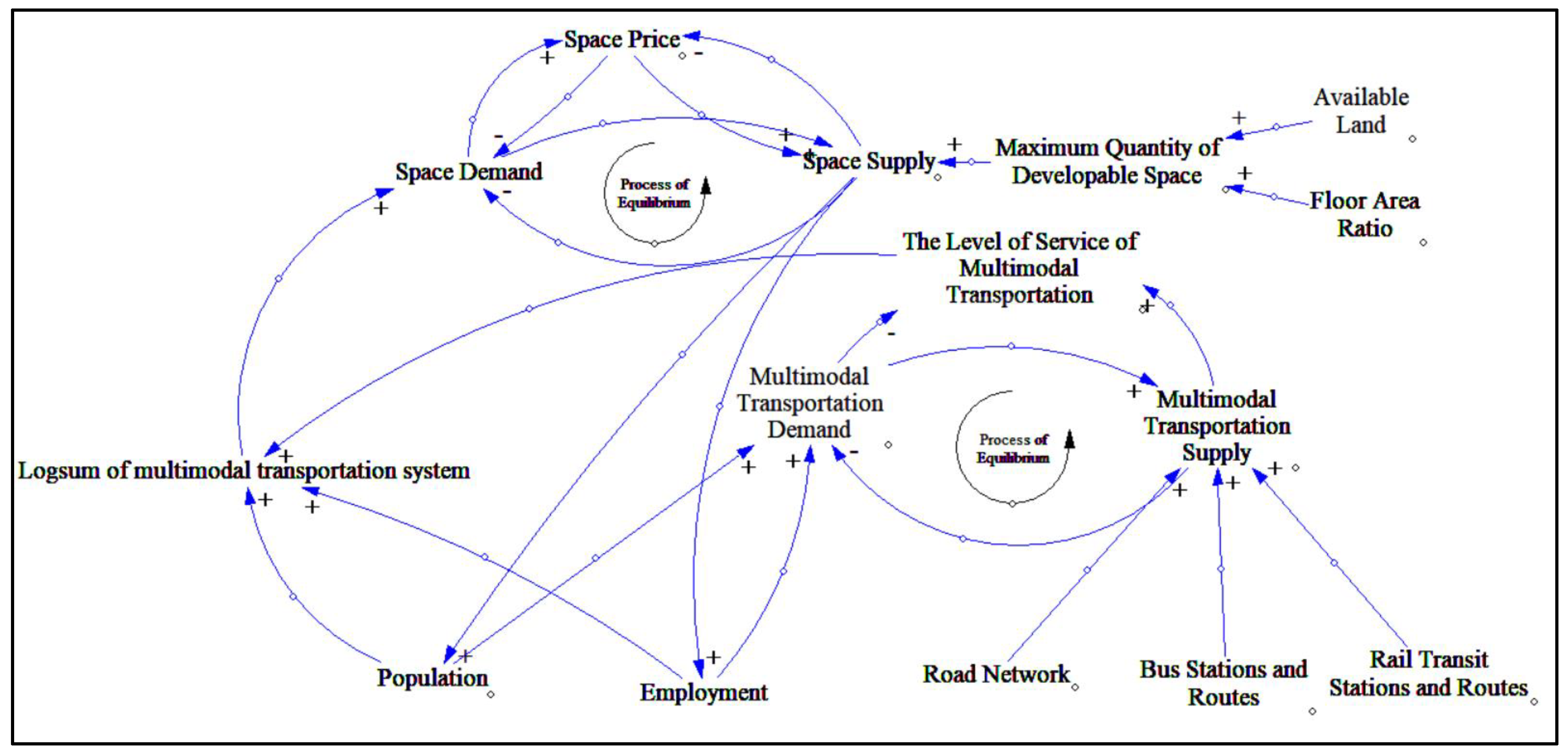
3.3.1. Analysis of the Causal Relationship between MLU and Transportation Supply Using a System Dynamics Diagram
- —
- Y represents the dependent variable;
- —
- represents the constant or intercept;
- —
- represents the estimated regression coefficient slope of the y regression on the independent variable ;
- —
- represents the independent variable or factors such as space price, space supply, population, employment, road network, bus stations and routes, and rail transit stations and routes, available land, and floor area ratio.
3.3.2. Parameters for Representing/Modeling MLU Patterns
- –
- is the maximum floor area ratio;
- –
- is the total floor area (m2) of the building ;
- –
- is the number of floors of the the building;
- –
- is the area of the parcels under calculation.
- –
- is the maximum developable space;
- –
- is the land use in the parcels i;
- –
- is the developable land of the parcel;
- –
- is the maximum floor area ratio.
- –
- represents the ratio of each type of land use;
- –
- represents the aggregate number of different types of land use in parcels .
- –
- represents the ratio of different types of land use within a parcel;
- –
- k represents the total number of different types of land use within a given parcel.
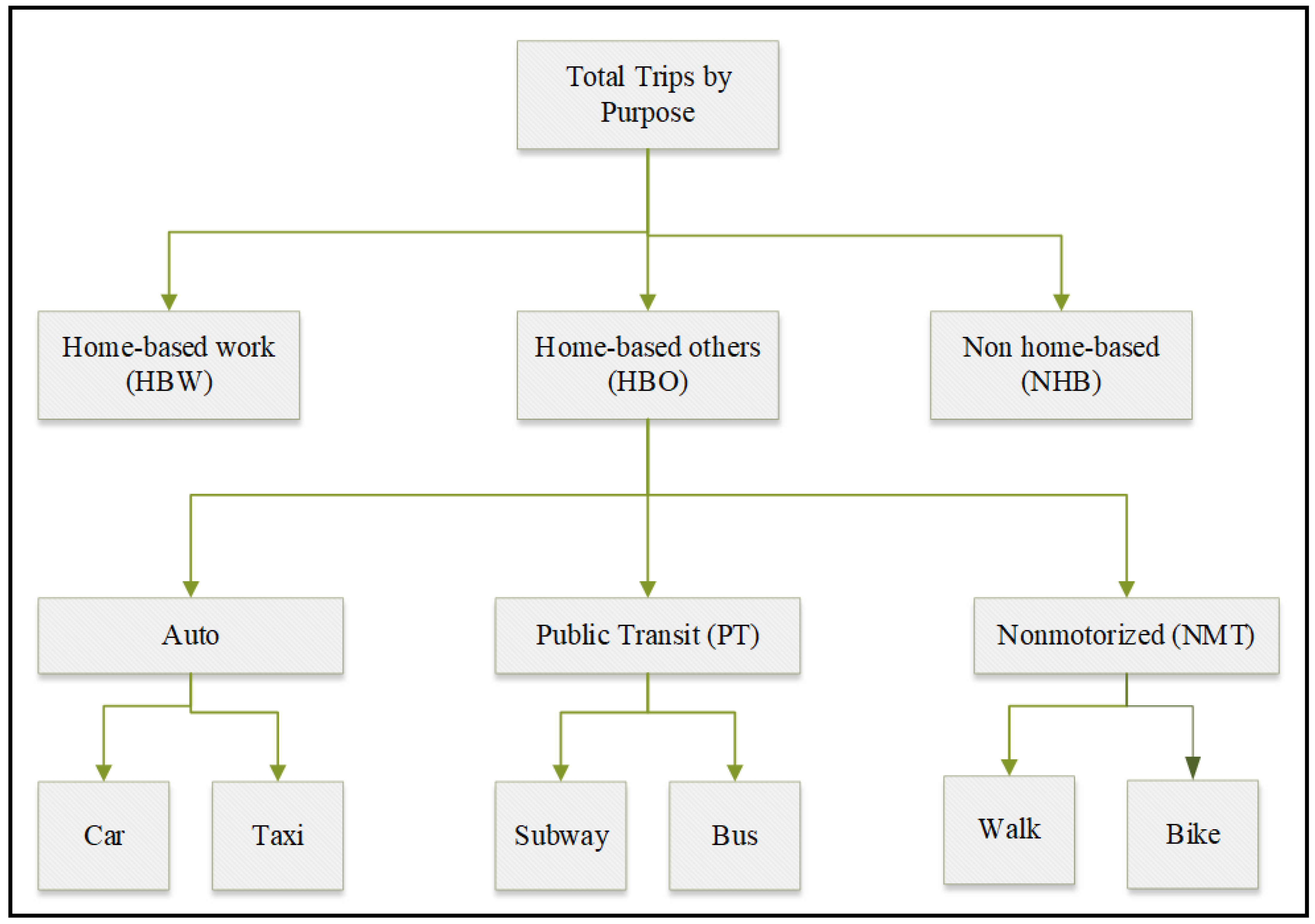
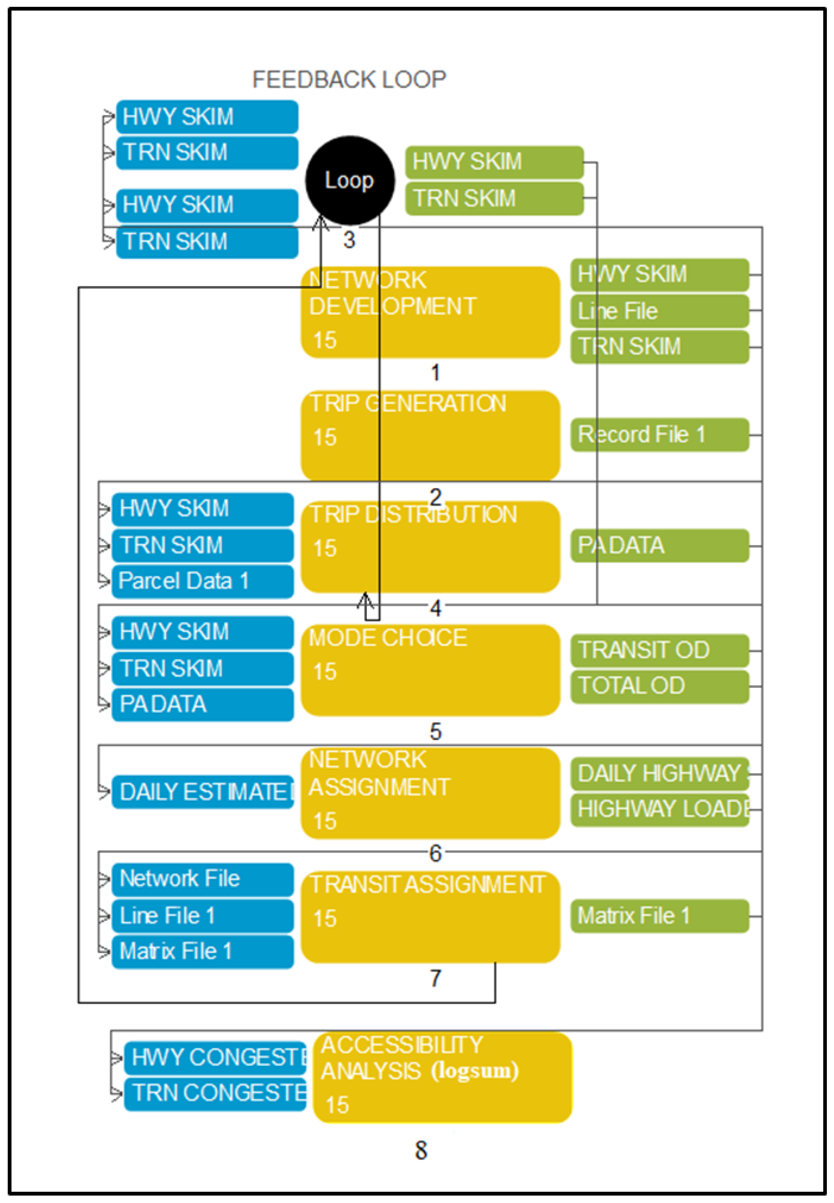
3.3.3. Transport Model
- (1)
- The trip generation module begins by estimating trip production and attraction rates using population, employment, and household data;
- (2)
- The trip distribution approach uses the gravity model to distribute these trips to every parcel;
- (3)
- A mode choice module: Transport utilities are calculated based on trip purposes (e.g., home-based work, home-based other, home-based school, and non-home-based) and transportation modes (including, bus, metro, bike, taxi, and personal car). These calculations are then incorporated into the nested logit model, as outlined in Table 4. The parameter β’s value fluctuates based on the trip purpose and the presence of a personal car. In this study, we specifically focus on trips related to home-based work and home-based other, both of which involve personal car usage. The attribute coefficients for various transportation modes, including in-vehicle time β1, waiting time β2, walking time β3, subway and bus fare β4, transfer time β5, β6, and cost per km by different trip purposes (HBW, HBO, HBS, and NHB), were obtained from the Wuhan Transportation Planning Institute (WHTPI) for different trip purposes (HBW, HBO, HBS, and NHB) (source: http://www.whtpi.com/Default.html, accessed on 15 April 2022).
- –
- TIV = In-Vehicle Time (actual time spent in the vehicle);
- –
- TIW = Initial Waiting Time at transit stations;
- –
- TW = Walking Time from home to transit stations, and waiting time in the case of a taxi; access time in the case of a car and bike;
- –
- FM = Metro Fare;
- –
- TMMT = Metro-to-Metro Transfer Time;
- –
- TMBT = Metro-to-Bus Transfer Time;
- –
- FB = Bus Fare;
- –
- TTT = Bus-to-Bus and Bus-to-Metro Transfer Time;
- –
- CD = Cost per Kilometer for driving a car.
- (4)
- The network assignment (user-equilibrium) and transit assignment (multi-routing) were developed to calculate congested travel time by all modes.
- (5)
- Furthermore, these measures are used to calculate the logsum of various modes (such as bike, bus, subway, car, and taxi), as shown in Equation (11).
- (6)
- Lastly, these data are utilized as independent variables in the MLP and LSTM approaches.
- –
- represents the logsum of parcel i;
- –
- i and j together represent the number of parcel;
- –
- k represents one of the transport modes;
- –
- n represents the total number of parcels;
- –
- m represents the total number of transport modes;
- –
- represents the utility produced by the transport mode k between parcel i and j.
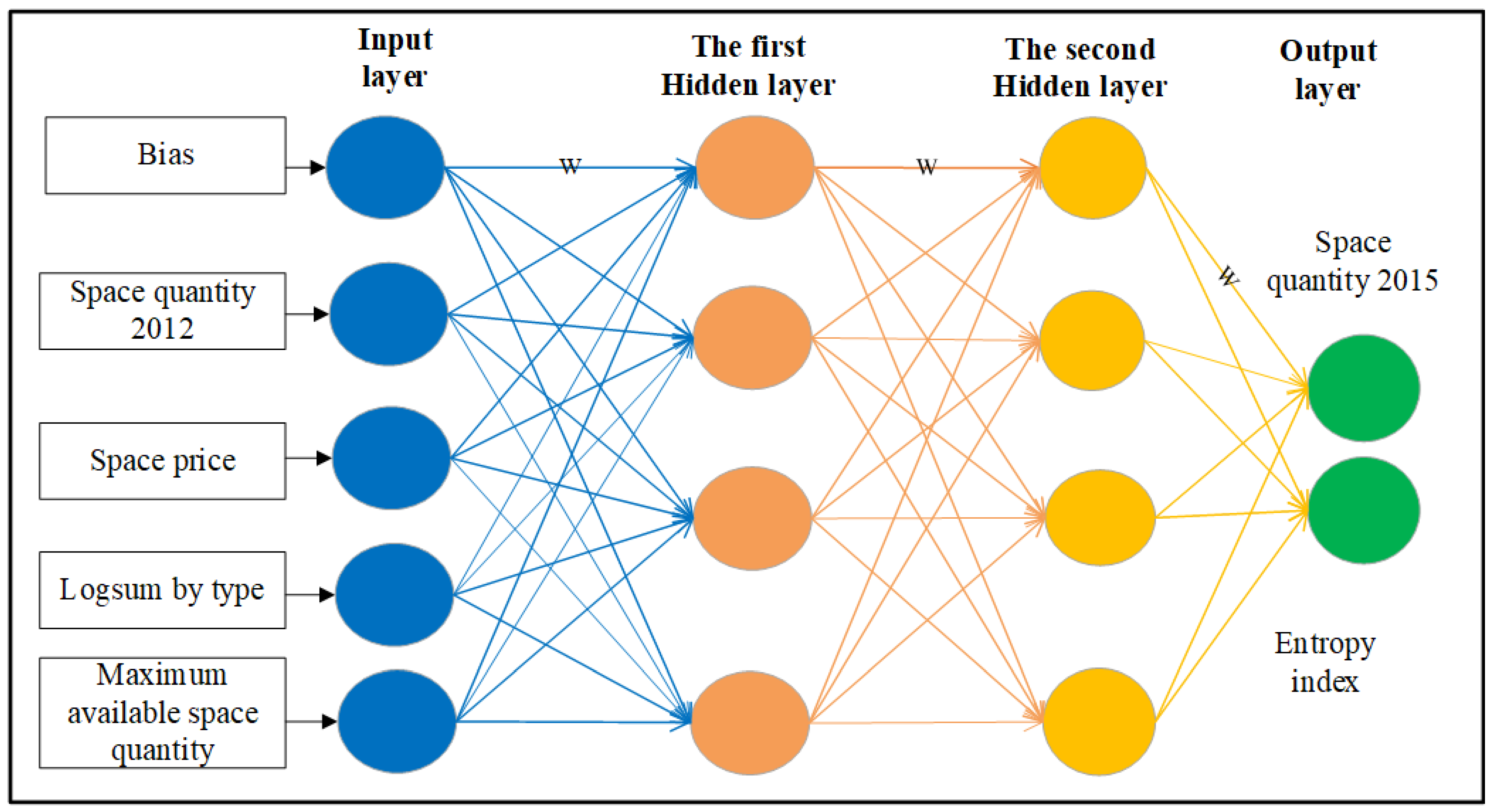
3.3.4. Multilayer Perceptron (MLP) Model
- –
- represents the neuron’s output value j;
- –
- represents the number of neurons in the previous layer;
- –
- represents the neuron’s i input value in space quantity for the year 2012, average floor price, logsum, etc;
- –
- represents the weight;
- –
- represents the bias;
- –
- represents the output following neuron j activation (the forecast of space quantity for 2015);
- –
- represents the activation function.
- –
- represent the tensors of arbitrary shapes with a total of n elements each;
- –
- The mean operation still operates over all the elements, and divides by N;
- –
- The division by N can be avoided if one sets reduction = ‘sum’.
- –
- represents mean relative error;
- –
- represents the total number of parcels i;
- –
- represents the predicted value;
- –
- represents the observed value.
3.3.5. Long Short-Term Memory (LSTM) Model
- –
- represents the input gate, and indicates cell activation;
- –
- denotes forget gate;
- –
- denotes the output gate, where refers to the sigmoid function;
- –
- denotes the weight, indicates bias;
- –
- represents cell state, and is the hidden state.
4. Results and Discussion
4.1. Results of the Causal Relationship between Transport Supply and MLU
- –
- represents the logsum of multimodal transportation system (MTS);
- –
- represents the population density;
- –
- represents the employment density;
- –
- represents the level of service of multimodal transportation;
- –
- represents the space price;
- –
- represents the space demand;
- –
- represents the space supply;
- –
- represents the multimodal transportation demand;
- –
- represents the multimodal transportation supply;
- –
- represents the road network;
- –
- represents the number of bus stations and routes;
- –
- represents the number of rail transit routes and stations;
- –
- represents the maximum quantity of developable space;
- –
- represents the available land;
- –
- represents the floor area ratio;
- –
- are the coefficients of the variables.
4.2. Logsum and MLU Change at the Parcel Level for the Years 2012 and 2015
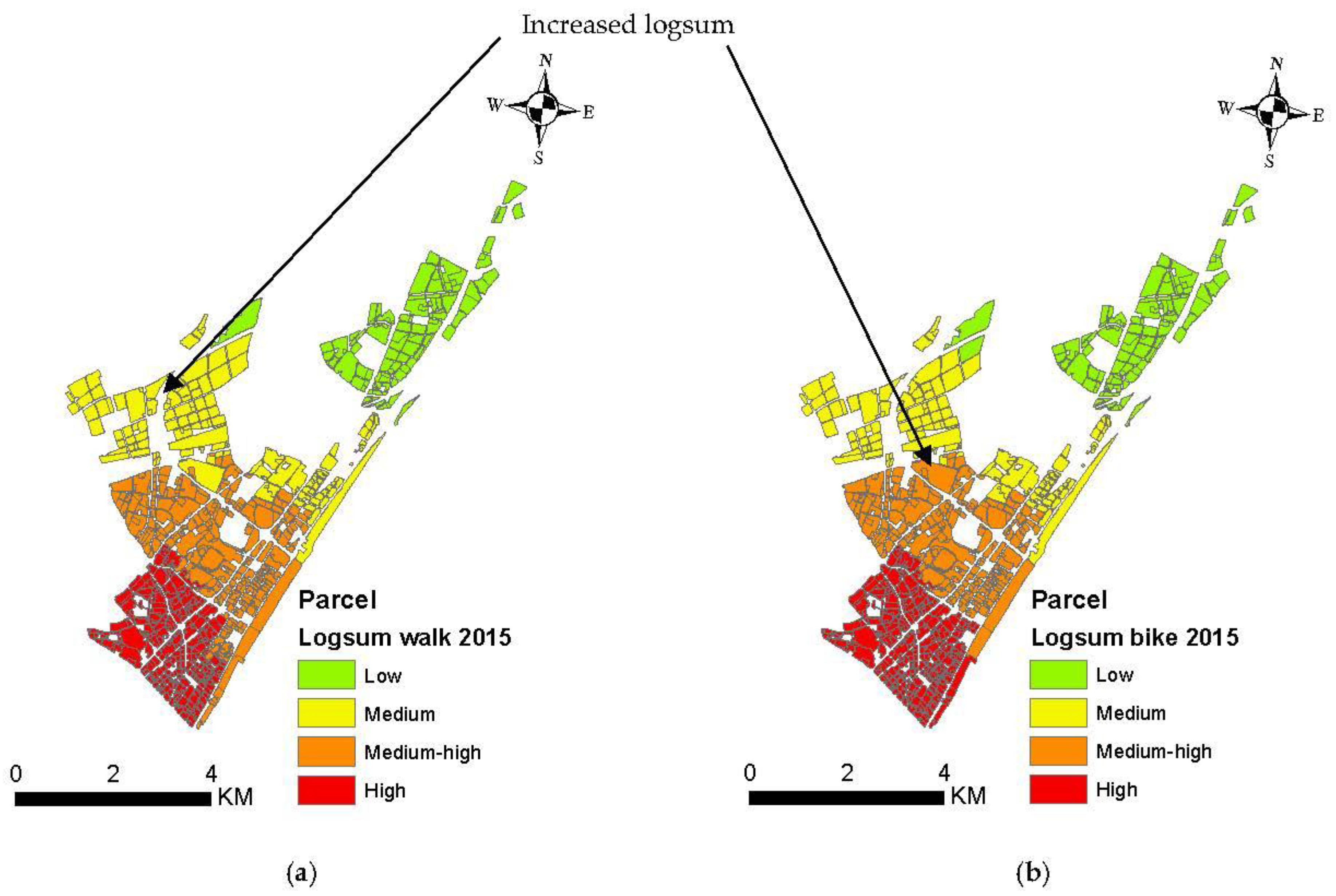
4.2.1. Logsum by Walk
4.2.2. Logsum by Bike
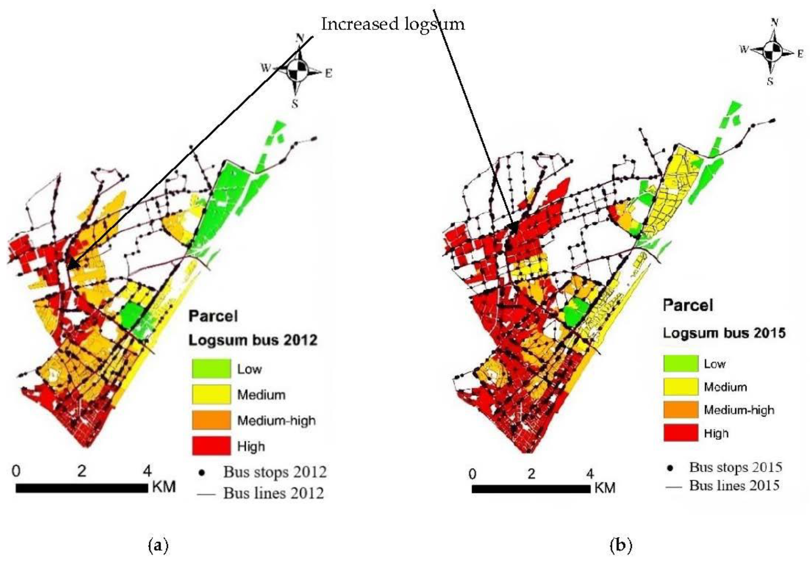
4.2.3. Logsum by Bus
4.2.4. Logsum by Subway
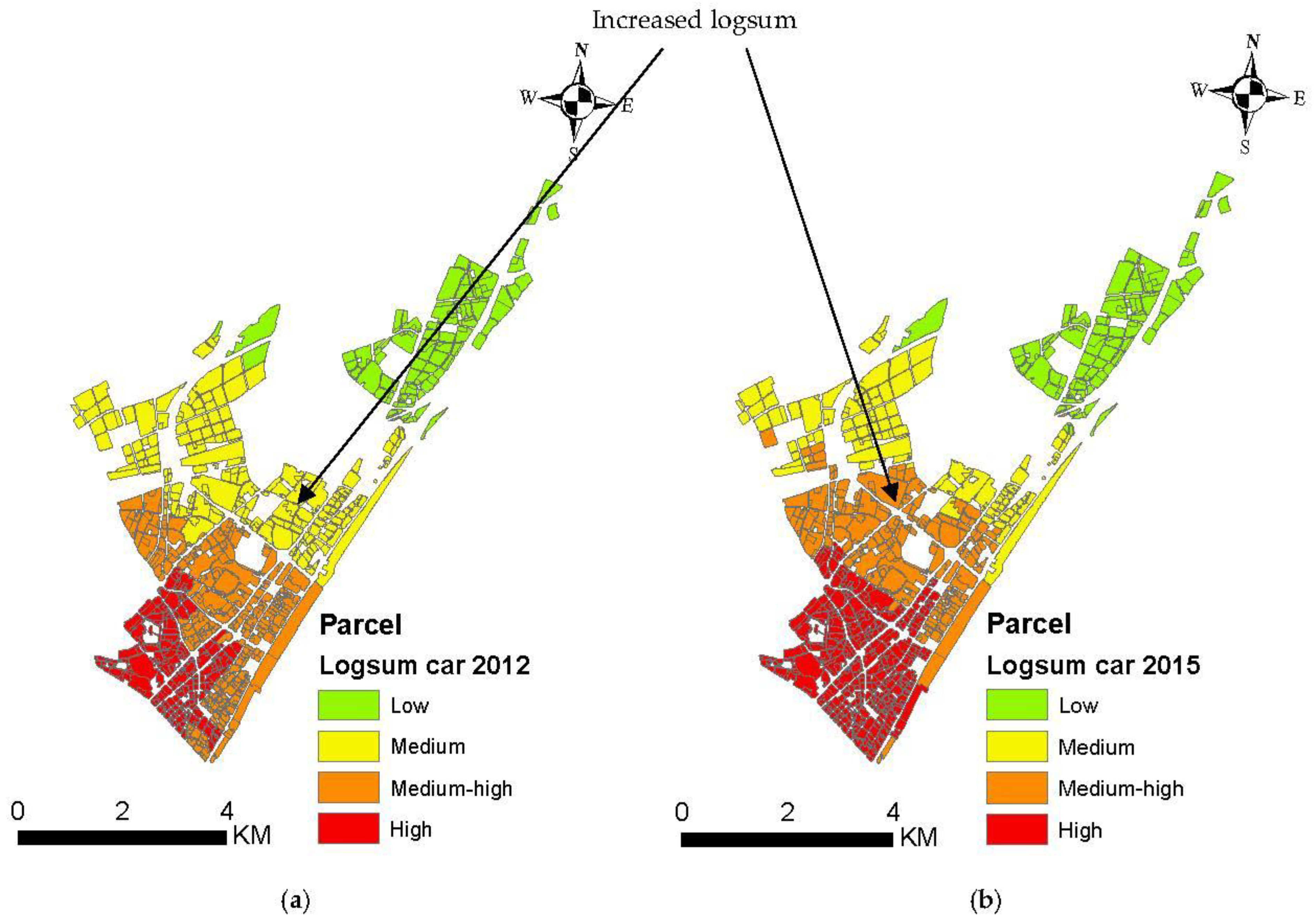
4.2.5. Logsum by Car
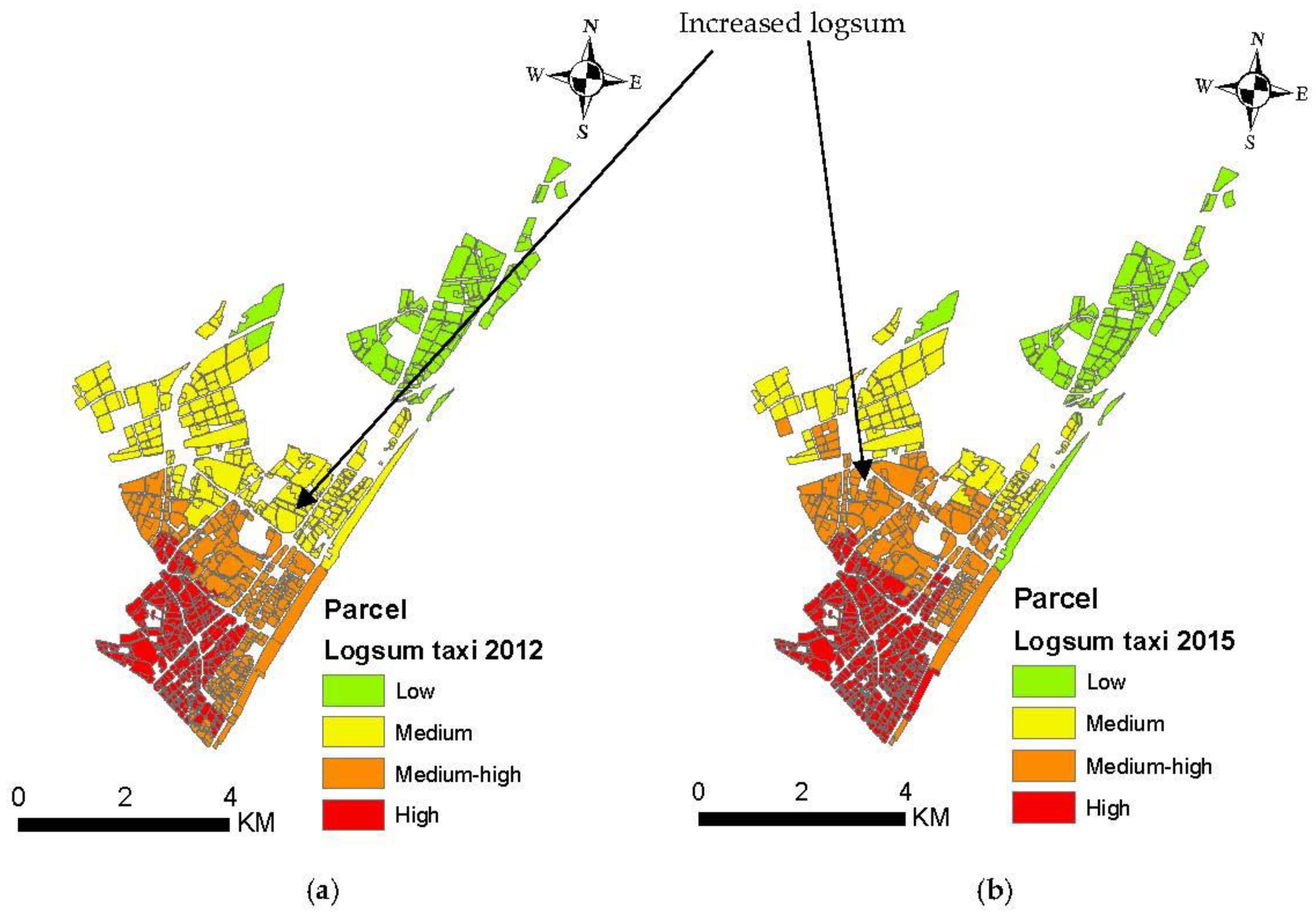
4.2.6. Logsum by Taxi
4.3. Parameter Settings and Model Training
4.4. Results of Prediction Accuracy of the MLP and LSTM Models and Their Comparative Analysis
4.5. Discussion
5. Conclusions and Recommendations
- –
- The study findings indicate significant changes in land use patterns, particularly in residential and mixed residential–commercial parcels, between 2012 and 2015. These changes were most pronounced in areas characterized by high logsum values under scenarios 3 (walk, bike, bus, subway) and 6 (walk, bus, car) in the central and southern regions of Jiang’an District. However, the amount of commercial and mixed commercial–residential area has increased primarily in the areas around the subway line 1 with a high logsum under scenario 7 (bike, subway, taxi). This implies that the increased logsum due to the supply of public transit under scenario 3 (walk, bike, bus, subway) and scenario 6 (walk, bus, car) encourages residential and mixed residential–commercial land development. Also, the increased logsum under scenario 7 (bike, subway, taxi) encourages commercial and mixed commercial–residential land development. The results from this study reinforced the conclusions from the previous studies that there is a strong relationship between transport supply and MLU.
- –
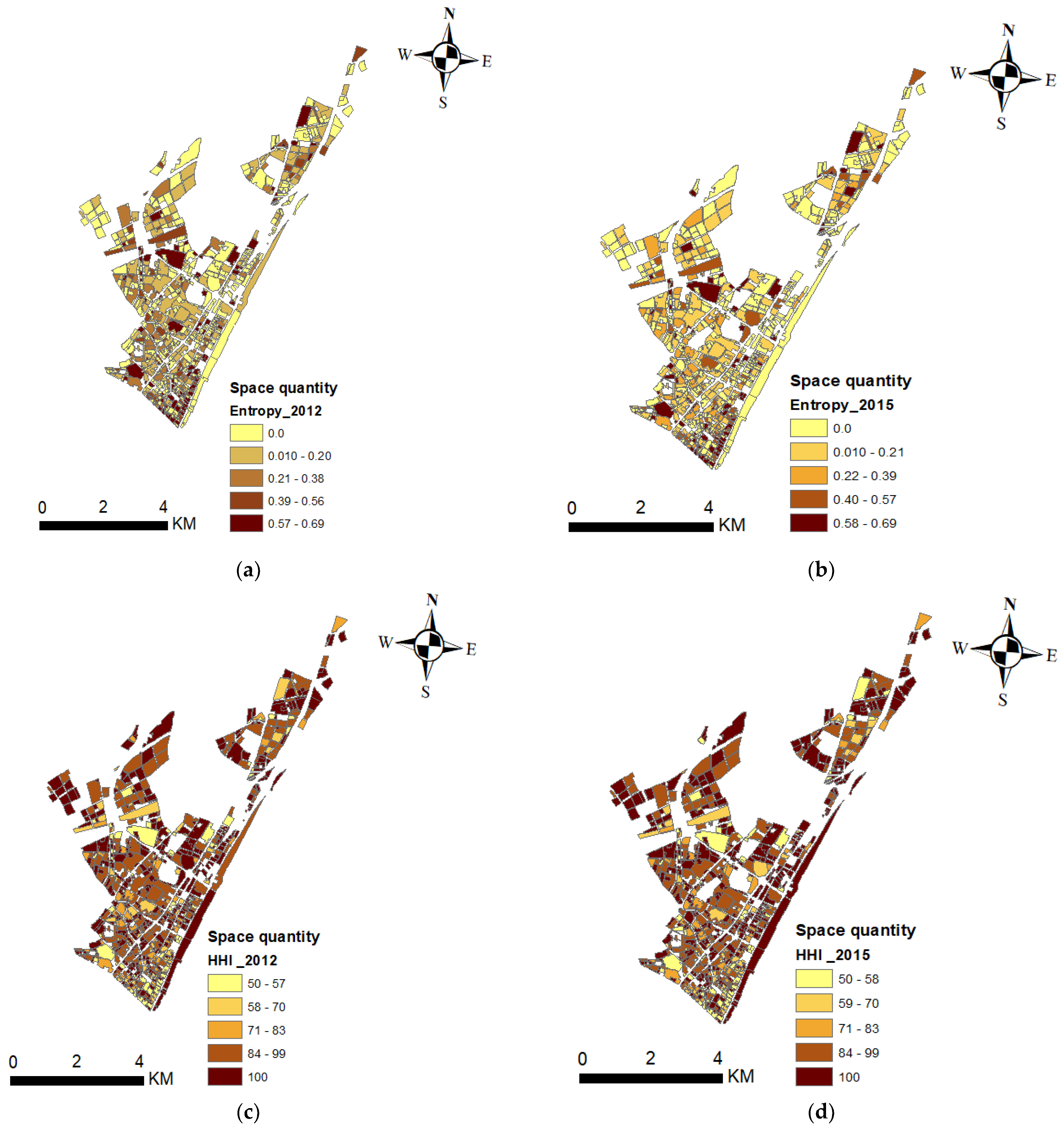
- The ENT and HH indexes, which are used to represent the level of MLU, show that the spatial distribution of a high and medium MLU density are increasingly found in downtown areas and around subway line 1, while areas farther away from the city center have a low MLU density for the years 2012 and 2015, suggesting that policies should be devised to enhance transport supply (represented by the logsum in the model) to encourage a high MLU density.
- –
- The MLP and LSTM model’s results indicated an MRE of 4.7–14.08%, and 3.74–10.38%, respectively. These findings indicate that the LSTM model outperforms the MLP model for all types of MLU.
- –
- This study employed a parcel-level disaggregated land use data to explore the relationship between transport supply and MLU patterns. This approach offers a nuanced understanding of land use dynamics, providing a more precise depiction of land development. Such detailed analysis significantly enhances the utility of the study’s findings in policy analysis. Using parcel-level data could help the government, stakeholders, and regional planning agencies in distributing measured demand across parcels in a manner reflective of differences in land use and intensity. With demand assigned to individual parcels, it is possible to determine the effects of a fluctuating transport supply on MLU. In fact, the method can be used to assess both new development plans and the existing urban fabric.
- –
- This paper employs real-world data and considers the case of a developing country to evaluate the relationship between transport supply and MLU. This will provide some guidelines and directions for the development of MLU and smart city in developing countries.
- –
- To promote and regulate MLU in urban zones, planners can develop a set of regulations regarding required transport supply measures. In addition, the technique can be applied to efficiently develop planning and land use regulations.
- –
- Examining the relationship between accessibility and MLU in urban settings empowers urban and transport planners to shape spatial conditions, fostering urban diversity, thereby contributing to desired sustainability. This approach not only guides the evolution of the city but also offers a framework for overseeing existing areas where MLU density requires management.
- –
- The study reveals that the density of MLU is intricately linked to the accessibility of subways and the city center. Consequently, effective planning and zoning regulations are essential to facilitate natural urban development instead of artificially dictating its form. Decision-makers can leverage these study findings to strategically intervene and realize the envisioned urban structure.
- –
- The study’s insights can be applied to model MLU based on specific accessibility scenarios. Moreover, it directly informs interventions in transport and town planning, aiding in understanding how changes in accessibility impact MLU. In essence, the study concludes that this serves as a valuable tool for decision-makers in town planning, land use planning, and transport planning, all aimed at achieving the overarching sustainability of future cities.
- –
- This study used advanced DNN techniques to predicts the impact of transportation-accessibility on MLU patterns at the parcel level. These insights empower long-term town planning through optimized urban predictions, informed accessibility planning, tailored policy formulation, and scenario modeling. By understanding the intricate relationship between accessibility and MLU density, decision-makers can guide sustainable urban growth, ensuring cities evolve harmoniously and inclusively.
Author Contributions
Funding
Institutional Review Board Statement
Informed Consent Statement
Data Availability Statement
Conflicts of Interest
References
- Safdar, M.; Jamal, A.; Al-Ahmadi, H.M.; Rahman, M.T.; Almoshaogeh, M. Analysis of the Influential Factors towards Adoption of Car-Sharing: A Case Study of a Megacity in a Developing Country. Sustainability 2022, 14, 2778. [Google Scholar] [CrossRef]
- Nabil, N.A.; Abd Eldayem, G.E. Influence of mixed land-use on realizing the social capital. HBRC J. 2015, 11, 285–298. [Google Scholar] [CrossRef]
- Knorre, A.; MacDonald, J. Shootings and land use. J. Crim. Justice 2023, 86, 102068. [Google Scholar] [CrossRef]
- Burton, E. Measuring Urban Compactness in UK Towns and Cities. Environ. Plan. B Plan. Des. 2002, 29, 219–250. [Google Scholar] [CrossRef]
- Association, A.P. Policy Guide on Smart Growth; The Association: Chicago, IL, USA, 2002. [Google Scholar]
- Sultana, S.; Powell, W.; Grant, J. Planning the Good Community: New Urbanism in Theory and Practice (review). Southeast. Geogr. 2009, 49, 308–312. [Google Scholar] [CrossRef]
- Shi, B.; Yang, J. Scale, distribution, and pattern of mixed land use in central districts: A case study of Nanjing, China. Habitat Int. 2015, 46, 166–177. [Google Scholar] [CrossRef]
- Yang, H.; Fu, M.; Wang, L.; Tang, F. Mixed Land Use Evaluation and Its Impact on Housing Prices in Beijing Based on Multi-Source Big Data. Land 2021, 10, 1103. [Google Scholar] [CrossRef]
- Choi, D.; Kang, M.; Yoon, J. Utility of mixed-use development by reducing aggregated travel time for multiple non-work activities: A case of Seoul, Korea. Cities 2021, 109, 103007. [Google Scholar] [CrossRef]
- Liang, X.; Guan, Q.F.; Clarke, K.C.; Chen, G.Z.; Guo, S.; Yao, Y. Mixed-cell cellular automata: A new approach for simulating the spatio-temporal dynamics of mixed land use structures. Landsc. Urban Plan. 2021, 205, 103960. [Google Scholar] [CrossRef]
- Wu, X.; Liu, X.; Zhang, D.; Zhang, J.; He, J.; Xu, X. Simulating mixed land-use change under multi-label concept by integrating a convolutional neural network and cellular automata: A case study of Huizhou, China. GIScience Remote Sens. 2022, 59, 609–632. [Google Scholar] [CrossRef]
- Jayasinghe, A.; Madusanka, N.B.S.; Abenayake, C.; Mahanama, P.K.S. A Modeling Framework: To Analyze the Relationship between Accessibility, Land Use and Densities in Urban Areas. Sustainability 2021, 13, 467. [Google Scholar] [CrossRef]
- Peng, Y.; Yamaguchi, H.; Funabora, Y.; Doki, S. Modeling Fabric-Type Actuator Using Point Clouds by Deep Learning. IEEE Access 2022, 10, 94363–94375. [Google Scholar] [CrossRef]
- Peng, Y.; Li, D.; Yang, X.; Ma, Z.; Mao, Z. A Review on Electrohydrodynamic (EHD) Pump. Micromachines 2023, 14, 321. [Google Scholar] [CrossRef] [PubMed]
- Wu, C.; Pei, Y.; Gao, J. Model for Estimation Urban Transportation Supply-Demand Ratio. Math. Probl. Eng. 2015, 2015, 502739. [Google Scholar] [CrossRef]
- Cao, R. Multi-Source Data Fusion for Land Use Classification Using Deep Learning. Ph.D. Thesis, University of Nottingham, Nottingham, UK, 2021. Available online: http://eprints.nottingham.ac.uk/63100/ (accessed on 5 October 2023).
- Kudas, D.; Wnęk, A.; Tátošová, L. Land Use Mix in Functional Urban Areas of Selected Central European Countries from 2006 to 2012. Int. J. Environ. Res. Public Health 2022, 19, 15233. [Google Scholar] [CrossRef] [PubMed]
- Ren, F.; Zhang, J.; Yang, X. Study on the Effect of Job Accessibility and Residential Location on Housing Occupancy Rate: A Case Study of Xiamen, China. Land 2023, 12, 912. [Google Scholar] [CrossRef]
- Li, J.; Huang, H. Effects of transit-oriented development (TOD) on housing prices: A case study in Wuhan, China. Res. Transp. Econ. 2020, 80, 100813. [Google Scholar] [CrossRef]
- Seong, E.Y.; Lee, N.H.; Choi, C.G. Relationship between Land Use Mix and Walking Choice in High-Density Cities: A Review of Walking in Seoul, South Korea. Sustainability 2021, 13, 810. [Google Scholar] [CrossRef]
- Kim, D.; Jin, J. The Effect of Land Use on Housing Price and Rent: Empirical Evidence of Job Accessibility and Mixed Land Use. Sustainability 2019, 11, 938. [Google Scholar] [CrossRef]
- Bhattacharjee, S.; Goetz, A.R. The rail transit system and land use change in the Denver metro region. J. Transp. Geogr. 2016, 54, 440–450. [Google Scholar] [CrossRef]
- Van Nes, A.; Berghauser Pont, M.; Mashhoodi, B. Combination of Space syntax with spacematrix and the mixed use index: The Rotterdam South test case. In Proceedings of the 8th International Space Syntax Symposium, Santiago de Chile, Chile, 3–6 January 2012; Available online: http://resolver.tudelft.nl/uuid:d865e5b6-519e-4959-8c3d-800054d1b351 (accessed on 20 October 2023).
- Koster, H.R.A.; Rouwendal, J. The Impact of Mixed Land Use on Residential Property Values*. J. Reg. Sci. 2012, 52, 733–761. [Google Scholar] [CrossRef]
- Maithani, S. A neural network based urban growth model of an Indian city. J. Indian Soc. Remote Sens. 2009, 37, 363–376. [Google Scholar] [CrossRef]
- Bivina, G.R.; Gupta, A.; Parida, M. Influence of microscale environmental factors on perceived walk accessibility to metro stations. Transp. Res. Part D Transp. Environ. 2019, 67, 142–155. [Google Scholar] [CrossRef]
- Munshi, T. Accessibility, Infrastructure Provision and Residential Land Value: Modelling the Relation Using Geographic Weighted Regression in the City of Rajkot, India. Sustainability 2020, 12, 8615. [Google Scholar] [CrossRef]
- Peng, Z.-R.; Zhao, L.-Y.; Yang, F. Development of a Prototype Land Use Model for Statewide Transportation Planning Activities; University of Florida: Gainesville, FL, USA, 2011. Available online: https://rosap.ntl.bts.gov/view/dot/23704 (accessed on 4 October 2023).
- Raman, R.; Roy, U.K. Taxonomy of urban mixed land use planning. Land Use Policy 2019, 88, 104102. [Google Scholar] [CrossRef]
- Almansoub, Y.; Zhong, M.; Raza, A.; Safdar, M.; Dahou, A.; Al-qaness, M.A.A. Exploring the Effects of Transportation Supply on Mixed Land-Use at the Parcel Level. Land 2022, 11, 797. [Google Scholar] [CrossRef]
- Raza, A.; Safdar, M.; Zhong, M.; Hunt, J.D. Analyzing Spatial Location Preference of Urban Activities with Mode-Dependent Accessibility Using Integrated Land Use–Transport Models. Land 2022, 11, 1139. [Google Scholar]
- Aygoren, S. Ins and Outs of Mixed-Use. Real Estate Forum 2004, 59, 66–71. Available online: https://www.cnu.org/sites/default/files/mixed_use_final_report_1-14-13_0.pdf (accessed on 3 October 2023).
- Hoppenbrouwer, E.; Louw, E. Mixed-use development: Theory and practice in Amsterdam’s Eastern Docklands. Eur. Plan. Stud. 2005, 13, 967–983. [Google Scholar] [CrossRef]
- Thwaites, K.; Porta, S.; Romice, O.; Greaves, M. Urban Sustainability through Environmental Design; Routledge: Abingdon, VA, USA, 2007; p. 166. Available online: https://www.planninginsights.co.in/data/ebook/1625738019.pdf (accessed on 20 October 2023).
- Maerten, A.-S.; Soydaner, D. From paintbrush to pixel: A review of deep neural networks in AI-generated art. arXiv 2023, arXiv:2302.10913. [Google Scholar] [CrossRef]
- Rodriguez-Conde, I.; Campos, C.; Fdez-Riverola, F. Horizontally Distributed Inference of Deep Neural Networks for AI-Enabled IoT. Sensors 2023, 23, 1911. [Google Scholar] [CrossRef] [PubMed]
- Lopez-Ballester, J.; Felici-Castell, S.; Segura Garcia, J.; Cobos, M. AI-IoT Platform for Blind Estimation of Room Acoustic Parameters Based on Deep Neural Networks. IEEE Internet Things J. 2022, 10, 855–866. [Google Scholar] [CrossRef]
- Omrani, H.; Tayyebi, A.; Pijanowski, B. Integrating the multi-label land-use concept and cellular automata with the artificial neural network-based Land Transformation Model: An integrated ML-CA-LTM modeling framework. GIScience Remote Sens. 2017, 54, 283–304. [Google Scholar] [CrossRef]
- Zhao, Y.; Lin, Q.W.; Ke, S.G.; Yu, Y.H. Impact of land use on bicycle usage: A big data-based spatial approach to inform transport planning. J. Transp. Land Use 2020, 13, 299–316. [Google Scholar] [CrossRef]
- Qin, Z.J.; Yu, Y.; Liu, D.F. The Effect of HOPSCA on Residential Property Values: Exploratory Findings from Wuhan, China. Sustainability 2019, 11, 471. [Google Scholar] [CrossRef]
- Kaeoruean, K.; Phithakkitnukoon, S.; Demissie, M.G.; Kattan, L.; Ratti, C. Analysis of demand–supply gaps in public transit systems based on census and GTFS data: A case study of Calgary, Canada. Public Transp. 2020, 12, 483–516. [Google Scholar] [CrossRef]
- Rad, T.G.; Alimohammadi, A. Modeling relationships between the network distance and travel time dynamics for assessing equity of accessibility to urban parks. Geo-Spat. Inf. Sci. 2021, 24, 509–526. [Google Scholar] [CrossRef]
- Sungwon, L.; Bumsoo, L. Comparing the impacts of local land use and urban spatial structure on household VMT and GHG emissions. J. Transp. Geogr. 2020, 84, 102694. [Google Scholar] [CrossRef]
- Jiao, J.C.; Rollo, J.; Fu, B.B. The Hidden Characteristics of Land-Use Mix Indices: An Overview and Validity Analysis Based on the Land Use in Melbourne, Australia. Sustainability 2021, 13, 1898. [Google Scholar] [CrossRef]
- Hu, W.; Dong, J.; Hwang, B.-g.; Ren, R.; Chen, Y.; Chen, Z. Using system dynamics to analyze the development of urban freight transportation system based on rail transit: A case study of Beijing. Sustain. Cities Soc. 2020, 53, 101923. [Google Scholar] [CrossRef]
- Fontoura, W.B.; Chaves, G.d.L.D.; Ribeiro, G.M. The Brazilian urban mobility policy: The impact in São Paulo transport system using system dynamics. Transp. Policy 2019, 73, 51–61. [Google Scholar] [CrossRef]
- Song, Y.; Merlin, L.; Rodriguez, D. Comparing measures of urban land use mix. Comput. Environ. Urban Syst. 2013, 42, 1–13. [Google Scholar] [CrossRef]
- Frank, L.D.; Schmid, T.L.; Sallis, J.F.; Chapman, J.; Saelens, B.E. Linking objectively measured physical activity with objectively measured urban form—Findings from SMARTRAQ. Am. J. Prev. Med. 2005, 28, 117–125. [Google Scholar] [CrossRef]
- Ienco, D.; Gaetano, R.; Dupaquier, C.; Maurel, P. Land Cover Classification via Multitemporal Spatial Data by Deep Recurrent Neural Networks. IEEE Geosci. Remote Sens. Lett. 2017, 14, 1685–1689. [Google Scholar] [CrossRef]
- Byeon, W.; Breuel, T.M.; Raue, F.; Liwicki, M. Scene labeling with lstm recurrent neural networks. In Proceedings of the IEEE Conference on Computer Vision and Pattern Recognition, Boston, MA, USA, 7–12 June 2015; pp. 3547–3555. [Google Scholar] [CrossRef]
- Shen, Q.; Chen, Q.; Tang, B.-s.; Yeung, S.; Hu, Y.; Cheung, G. A system dynamics model for the sustainable land use planning and development. Habitat Int. 2009, 33, 15–25. [Google Scholar] [CrossRef]
- Priyadarisini, K.D.; Umadevi, G. A System Dynamics Model for Assessing Land-Use Transport Interaction Scenarios in Chennai, India. Sustainability 2023, 15, 6297. [Google Scholar] [CrossRef]
- He, C.; Shi, P.; Chen, J.; Li, X.; Pan, Y.; Li, J.; Li, Y.; Li, J. Developing land use scenario dynamics model by the integration of system dynamics model and cellular automata model. Sci. China Ser. D Earth Sci. 2005, 48, 1979–1989. [Google Scholar] [CrossRef]
- Haghani, A.; Lee, S.Y.; Byun, J.H. A system dynamics approach to land use/transportation system performance modeling Part II: Application. J. Adv. Transp. 2003, 37, 43–82. [Google Scholar] [CrossRef]
- Noviandi, N.; Pradono, P.; Tasrif, M.; Kusumantoro, I.P. Modeling of dynamics complexity of land use and transport in megapolitan urban fringe (case of Bekasi city). Transp. Res. Procedia 2017, 25, 3314–3332. [Google Scholar] [CrossRef]
- He, J.; Li, X.; Liu, P.; Wu, X.; Zhang, J.; Zhang, D.; Liu, X.; Yao, Y. Accurate Estimation of the Proportion of Mixed Land Use at the Street-Block Level by Integrating High Spatial Resolution Images and Geospatial Big Data. IEEE Trans. Geosci. Remote Sens. 2021, 59, 6357–6370. [Google Scholar] [CrossRef]


| Years | Bus Lines | Subway Stations | Population (Persons) | Parcels (Nos) |
|---|---|---|---|---|
| 2012 | 141 | 12 | 921,700 | 871 |
| 2015 | 196 | 14 | 954,300 |
| Years/Type | 2012 | 2015 | ||
|---|---|---|---|---|
| Total Space Quantity | Average Floor Space Price | Total Space Quantity | Average Floor Space Price | |
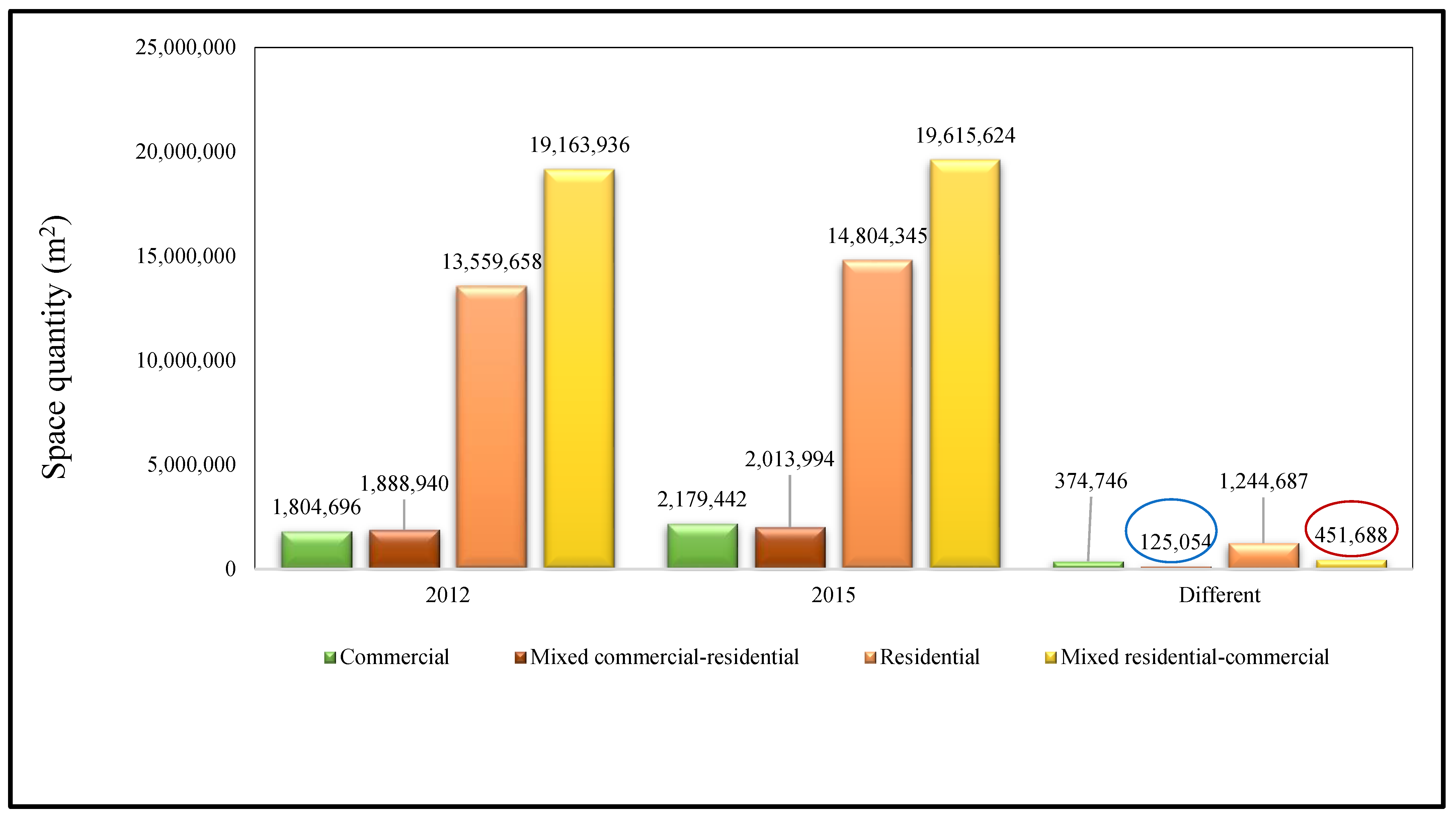
| Commercial | 1,804,696 | 18,934 | 2,179,442 | 22,853 |
| Mix (Commercial–Residential) | 1,888,940 | 16,791 | 2,013,994 | 20,579 |
| Residential | 13,559,658 | 8027 | 14,804,345 | 10,749 |
| Mix (Residential–Commercial) | 19,163,936 | 9704 | 19,615,624 | 12,649 |
| Total Space Quantity | 36,417,230 | - | 38,613,405 | - |
| Land Use Type | 2012 | 2015 | ||
|---|---|---|---|---|
| Number of Locations | Average Price | Number of Locations | Average Price | |
| Residential prices | 72 | 8150 | 90 | 9901 |
| Commercial prices | 20 | 18,640 | 30 | 19,294 |
| Home-Based Work (HBW) Car Available | Home-Based Other (HBO) Car Available | |||||||||||
|---|---|---|---|---|---|---|---|---|---|---|---|---|
| Modes | 1 | 2 | 3 | 4 | 5 | 6 | β1 | β2 | β3 | β4 | β5 | β6 |
| Metro | −0.02 | −0.04 | −0.04 | −0.039 | −0.1 | −0.2 | −0.02 | −0.04 | −0.04 | −0.078 | −0.1 | −0.2 |
| Bus | −0.02 | −0.04 | −0.04 | −0.039 | −0.2 | −0.02 | −0.04 | −0.04 | −0.078 | −0.2 | ||
| Taxi | −0.02 | −0.04 | −0.039 | −0.02 | −0.04 | −0.078 | ||||||
| Car | −0.02 | −0.04 | −0.039 | −0.02 | −0.04 | −0.078 | ||||||
| Bike | −0.02 | −0.04 | −0.02 | −0.04 | ||||||||
| Home-based school (HBS) | Non-home-based (NHB) | |||||||||||
| Modes | β1 | β2 | β3 | β4 | β5 | β6 | β1 | β2 | β3 | β4 | β5 | β6 |
| Metro | −0.02 | −0.04 | −0.04 | −0.305 | −0.1 | −0.2 | −0.02 | −0.04 | −0.04 | −0.114 | −0.1 | −0.2 |
| Bus | −0.02 | −0.04 | −0.04 | −0.305 | −0.2 | −0.02 | −0.04 | −0.04 | −0.114 | −0.2 | ||
| Taxi | −0.02 | −0.04 | −0.305 | −0.02 | −0.04 | −0.114 | ||||||
| Car | −0.02 | −0.04 | −0.305 | −0.02 | −0.04 | −0.114 | ||||||
| Bike | −0.02 | −0.04 | −0.02 | −0.04 | ||||||||
| No | Pearson Correlation | (1) | (2) | (3) | (4) | (5) | (6) | (7) | (8) | (9) | (10) | (11) | (12) | (13) | (14) | (15) |
|---|---|---|---|---|---|---|---|---|---|---|---|---|---|---|---|---|
| (1) | Commercial Space (CS) 2012 | 1 | ||||||||||||||
| (2) | Commercial–Residential Space (CRS) 2012 | −0.050 | 1 | |||||||||||||
| (3) | Residential Space (RS) 2012 | −0.063 * | −0.082 ** | 1 | ||||||||||||
| (4) | Residential–Commercial Space (RCS) 2012 | −0.074 * | −0.096 ** | −0.122 ** | 1 | |||||||||||
| (5) | Commercial Space (CS) 2015 | 0.835 ** | −0.042 | −0.063 * | −0.074 * | 1 | ||||||||||
| (6) | Commercial–Residential Space (CRS) 2015 | −0.042 | 0.924 ** | −0.084 ** | −0.092 ** | −0.051 | 1 | |||||||||
| (7) | Residential Space (RS) 2015 | −0.063 * | −0.082 ** | .914 ** | −0.107 ** | −0.063 * | −0.084 ** | 1 | ||||||||
| (8) | Residential–Commercial Space (RCS) 2015 | −0.075 * | −0.090 ** | −0.103 ** | 0.965 ** | −0.075 * | −0.100 ** | −0.124 ** | 1 | |||||||
| (9) | Logsum Walk 2015 | 0.044 | 0.051 | −0.046 | −0.015 | 0.041 | 0.053 | −0.046 | −0.014 | 1 | ||||||
| (10) | Logsum Bik 2015 | 0.027 | 0.031 | −0.001 | −0.011 | 0.025 | 0.032 | 0.001 | −0.010 | 0.939 ** | 1 | |||||
| (11) | Logsum Bus 2015 | 0.038 | 0.049 | −0.026 | −0.018 | 0.034 | 0.048 | −0.012 | −0.016 | 0.712 ** | 0.667 ** | 1 | ||||
| (12) | Logsum Subway 2015 | 0.008 | 0.058 * | −0.077 * | −0.069 * | −0.008 | 0.051 | −0.095 ** | −0.078 * | 0.499 ** | 0.537 ** | 0.247 ** | 1 | |||
| (13) | Max Available Space | −0.045 | −0.062 * | 0.260 ** | 0.437 ** | −0.051 | −0.067 * | 0.280 ** | 0.447 ** | −0.034 | 0.082 ** | −0.040 | −0.167 ** | 1 | ||
| (14) | Residential Price 2015 (RP) | 0.004 | 0.172 ** | −0.185 * | −0.170 * | 0.003 | 0.041 | −0.112 * | −0.247 ** | 0.168 ** | 0.156 ** | 0.178 ** | 0.074 * | −0.463 ** | 1 | |
| (15) | Commercial Price 2015 (CP) | 0.130 | 0.052 | −0.106 * | −0.219 ** | 0.031 | 0.051 | 0.023 | 0.040 | 0.108 ** | 0.058 * | 0.335 ** | 0.335 ** | −0.285 ** | 0.748 ** | 1 |
| Model | Dependent Variables | R Square | Adjusted R Square | Std. Error of the Estimate |
|---|---|---|---|---|
| 1 | Logsum by MTS | 0.66 | 0.65 | 1.26 |
| 2 | Space Demand | 0.75 | 0.75 | 0.59 |
| 3 | Multimodal Transportation Demand | 0.62 | 0.60 | 1.15 |
| 4 | Multimodal Transportation Supply | 0.72 | 0.70 | 0.96 |
| 5 | Maximum Quantity of Developable Space | 0.68 | 0.66 | 1.03 |
| Dependent Variables | Independent Variables | Unstandardized Coefficients | Standardized Coefficients | t-Values | Significance (p-Values) | ||
|---|---|---|---|---|---|---|---|
| B | Beta | Beta | |||||
| 1 | Logsum by MTS | Population | 1.36 | 0.09 | 0.78 | 14.98 | 0.00 |
| Employment | 1.17 | 0.03 | 0.82 | 38.73 | 0.00 | ||
| The Level of Service of Multimodal Transportation | 0.85 | 0.10 | 0.49 | 8.41 | 0.00 | ||
| 2 | Space Demand | Space Price | 0.94 | 0.11 | 0.54 | 8.96 | 0.00 |
| Space Supply | 4.70 | 0.77 | 0.37 | 6.11 | 0.00 | ||
| Logsum by car | 3.81 | 0.75 | 0.30 | 5.10 | 0.00 | ||
| 3 | Multimodal Transportation Demand | Population | 0.93 | 0.03 | 0.65 | 13.14 | 0.00 |
| Employment | 0.31 | 0.07 | 0.23 | 30.55 | 0.00 | ||
| Multimodal Transportation Supply | 1.86 | 0.47 | 0.36 | 3.98 | 0.00 | ||
| 4 | Multimodal Transportation Supply | Road Network | 3.81 | 0.75 | 0.30 | 5.10 | 0.00 |
| Bus Stations and Routes | 4.00 | 0.38 | 0.24 | 10.46 | 0.00 | ||
| Rail Transit Stations and Routes | 0.80 | 0.03 | 0.56 | 23.91 | 0.00 | ||
| 5 | Maximum Quantity of Developable Space | Available Land | 0.31 | 0.07 | 0.23 | 4.55 | 0.00 |
| Floor Area Ratio | 3.81 | 0.75 | 0.30 | 5.10 | 0.00 | ||
| Total of Space Quantity Change (m2) | |||||
|---|---|---|---|---|---|
| Years/Type | C | CR | R | RC | Total Space |
| Total space quantity 2012 | 1,804,696 | 1,888,940 | 13,559,658 | 19,163,936 | 36,417,230 |
| Total space quantity 2015 | 2,179,442 | 2,013,994 | 14,804,345 | 19,615,624 | 38,613,405 |
| Total change | 374,746 | 125,054 | 1,244,687 | 451,688 | 2,196,175 |
| Input Variables for Training (70% of Data Samples) | Output Variables for Training (70% of Data Samples) | Input Variables for Testing (30% of Data Samples) | Output Variables for Testing (30% of Data Samples) |
|---|---|---|---|
| Average floor space price by types (2012, 2015) | Space quantity in 2015, ENT index | Average floor space price by types (2012, 2015) | Space quantity in 2015, ENT index |
| Maximum available space quantity | Maximum available space quantity | ||
| Space quantity in 2012 | Space quantity in 2012 | ||
| Logsum by type (2012, 2015) | Logsum by type (2012, 2015) |
| Mode /Scenario | Nonmotorized (Nmt) | Public Transit (Pt) | Auto | |||
|---|---|---|---|---|---|---|
| Scenario 1 (All modes separated) | Walk | Bike | Bus | Subway | Car | Taxi |
| Scenario 2 (All modes together) | Walk | Bike | Bus | Subway | Car | Taxi |
| Scenario 3 | Walk | Bike | Bus | Subway | --- | --- |
| Scenario 4 | --- | --- | Bus | Subway | Car | Taxi |
| Scenario 5 | Walk | Bike | --- | --- | Car | Taxi |
| Scenario 6 | Walk | --- | Bus | --- | Car | --- |
| Scenario 7 | --- | Bike | --- | Subway | --- | Taxi |
| Models | MLP Training Errors (%) | LSTM Training Errors (%) | |||||||||||
|---|---|---|---|---|---|---|---|---|---|---|---|---|---|
| Scenario\Land Type | Mixed CR | Mixed RC | Mixed CR | Mixed RC | |||||||||
| MRE (%) | MRE (%) | MRE (%) | MRE(%) | ||||||||||
| C | R | CR | C | R | RC | C | R | CR | C | R | RC | ||
| Scenario 1 | Walk | 1.35 | 0.97 | 2.32 | 0.85 | 1.32 | 2.17 | 1.97 | 1.64 | 3.61 | 1.11 | 1.65 | 2.76 |
| Bike | 1.36 | 0.97 | 2.33 | 0.84 | 1.31 | 2.15 | 1.99 | 1.66 | 3.65 | 1.12 | 1.66 | 2.78 | |
| Bus | 1.12 | 0.80 | 1.92 | 0.76 | 1.18 | 1.94 | 1.99 | 1.66 | 3.65 | 1.14 | 1.69 | 2.83 | |
| Subway | 1.34 | 0.96 | 2.30 | 0.74 | 1.15 | 1.89 | 1.78 | 1.48 | 3.26 | 1.10 | 1.64 | 2.74 | |
| Car | 1.35 | 0.97 | 2.32 | 0.83 | 1.30 | 2.13 | 2.07 | 1.72 | 3.79 | 1.12 | 1.67 | 2.79 | |
| Taxi | 1.36 | 0.97 | 2.33 | 0.84 | 1.31 | 2.15 | 2.02 | 1.68 | 3.70 | 1.13 | 1.68 | 2.81 | |
| Scenario 2 | 1.50 | 1.08 | 2.58 | 0.69 | 1.08 | 1.77 | 2.00 | 1.67 | 3.67 | 1.1 | 1.66 | 2.76 | |
| Scenario 3 | 2.16 | 1.54 | 3.70 | 0.67 | 1.05 | 1.72 | 1.98 | 1.65 | 3.63 | 1.12 | 1.66 | 2.78 | |
| Scenario 4 | 1.06 | 0.76 | 1.82 | 0.70 | 1.09 | 1.79 | 1.58 | 1.32 | 2.9 | 1.14 | 1.69 | 2.83 | |
| Scenario 5 | 0.83 | 0.59 | 1.42 | 1.08 | 1.69 | 2.77 | 2.12 | 1.76 | 3.88 | 1.11 | 1.64 | 2.75 | |
| Scenario 6 | 1.41 | 1.00 | 2.41 | 0.69 | 1.08 | 1.77 | 1.46 | 1.22 | 2.68 | 1.12 | 1.68 | 2.8 | |
| Scenario 7 | 1.28 | 0.92 | 2.20 | 0.71 | 1.12 | 1.83 | 2.04 | 1.70 | 3.74 | 1.09 | 1.62 | 2.71 | |
| Models | MLP Testing Errors (%) | LSTM Testing Errors (%) | |||||||||||
|---|---|---|---|---|---|---|---|---|---|---|---|---|---|
| MRE | Mixed CR | Mixed RC | Mixed CR | Mixed RC | |||||||||
| MRE (%) | MRE (%) | MRE (%) | MRE (%) | ||||||||||
| Scenario\Land Type | C | R | CR | C | R | RC | C | R | CR | C | R | RC | |
| Scenario 1 | Walk | 5.61 | 3.50 | 9.11 | 3.57 | 2.61 | 6.18 | 4.43 | 3.09 | 7.52 | 1.7 | 2.30 | 4 |
| Bike | 5.57 | 3.48 | 9.05 | 3.43 | 2.50 | 5.93 | 4.34 | 3.03 | 7.37 | 1.80 | 2.30 | 4.10 | |
| Bus | 5.25 | 3.28 | 8.53 | 3.52 | 2.57 | 6.09 | 5.58 | 3.89 | 9.47 | 1.72 | 2.20 | 3.92 | |
| Subway | 5.80 | 3.62 | 9.42 | 3.55 | 2.59 | 6.14 | 5.58 | 3.89 | 9.47 | 1.81 | 2.31 | 4.12 | |
| Car | 5.54 | 3.46 | 9.00 | 3.51 | 2.56 | 6.07 | 4.49 | 3.14 | 7.63 | 1.85 | 2.36 | 4.21 | |
| Taxi | 5.51 | 3.44 | 8.95 | 3.48 | 2.54 | 6.02 | 4.39 | 3.07 | 7.46 | 1.85 | 2.37 | 4.22 | |
| Scenario 2 | 5.90 | 3.69 | 9.59 | 2.78 | 2.03 | 4.81 | 4.76 | 3.32 | 8.08 | 1.93 | 2.47 | 4.40 | |
| Scenario 3 | 8.67 | 5.41 | 14.08 | 2.72 | 1.98 | 4.70 | 5.54 | 3.87 | 9.41 | 1.94 | 2.48 | 4.42 | |
| Scenario 4 | 7.76 | 4.85 | 12.61 | 2.74 | 2.00 | 4.74 | 5.10 | 3.56 | 8.66 | 2.00 | 2.55 | 4.55 | |
| Scenario 5 | 6.29 | 3.92 | 10.21 | 3.16 | 2.31 | 5.47 | 6.11 | 4.27 | 10.38 | 1.92 | 2.45 | 4.37 | |
| Scenario 6 | 4.79 | 2.99 | 7.78 | 2.87 | 2.09 | 4.96 | 4.59 | 3.20 | 7.79 | 1.64 | 2.10 | 3.74 | |
| Scenario 7 | 4.49 | 2.81 | 7.30 | 3.02 | 2.20 | 5.22 | 4.19 | 2.92 | 7.11 | 2.01 | 2.57 | 4.58 | |
| Authors | Objectives | Methodology | City/ Country | MRE |
|---|---|---|---|---|
| Jayasinghe et al. [12] | Analyze the relationship between accessibility, MLU, and densities | Decision tree | Srilanka | 20% |
| Yang et al. [8] | Explore the impact of accessibility and MLU on housing price | MGWR | Beijing, China | 17.33% |
| Wu et al. [11] | A study on cellular automata with machine learning to simulate MLU changes | (ML-CNN-CA) | Huizhou, China | 9–11% |
| He et al. [56] | Estimate the percentage of MLU changes using DNN (CNN) | (CF-CNN), (SRes-Net), (PVGG-Net) | Guangzhou, China | 6%, 8.3%, and 10% |
| The proposed model of the current study | Evaluate the effect of transport supply on MLU at the parcel level | MLP and LSTM | Wuhan, China | 4.7–14.08% and 3.74–10.38% |
Disclaimer/Publisher’s Note: The statements, opinions and data contained in all publications are solely those of the individual author(s) and contributor(s) and not of MDPI and/or the editor(s). MDPI and/or the editor(s) disclaim responsibility for any injury to people or property resulting from any ideas, methods, instructions or products referred to in the content. |
© 2023 by the authors. Licensee MDPI, Basel, Switzerland. This article is an open access article distributed under the terms and conditions of the Creative Commons Attribution (CC BY) license (https://creativecommons.org/licenses/by/4.0/).
Share and Cite
Almansoub, Y.; Zhong, M.; Safdar, M.; Raza, A.; Dahou, A.; Al-qaness, M.A.A. Modeling Impact of Transportation Infrastructure-Based Accessibility on the Development of Mixed Land Use Using Deep Neural Networks: Evidence from Jiang’an District, City of Wuhan, China. Sustainability 2023, 15, 15470. https://doi.org/10.3390/su152115470
Almansoub Y, Zhong M, Safdar M, Raza A, Dahou A, Al-qaness MAA. Modeling Impact of Transportation Infrastructure-Based Accessibility on the Development of Mixed Land Use Using Deep Neural Networks: Evidence from Jiang’an District, City of Wuhan, China. Sustainability. 2023; 15(21):15470. https://doi.org/10.3390/su152115470
Chicago/Turabian StyleAlmansoub, Yunes, Ming Zhong, Muhammad Safdar, Asif Raza, Abdelghani Dahou, and Mohammed A. A. Al-qaness. 2023. "Modeling Impact of Transportation Infrastructure-Based Accessibility on the Development of Mixed Land Use Using Deep Neural Networks: Evidence from Jiang’an District, City of Wuhan, China" Sustainability 15, no. 21: 15470. https://doi.org/10.3390/su152115470
APA StyleAlmansoub, Y., Zhong, M., Safdar, M., Raza, A., Dahou, A., & Al-qaness, M. A. A. (2023). Modeling Impact of Transportation Infrastructure-Based Accessibility on the Development of Mixed Land Use Using Deep Neural Networks: Evidence from Jiang’an District, City of Wuhan, China. Sustainability, 15(21), 15470. https://doi.org/10.3390/su152115470