Joint Optimization of Distance-Based Fares and Headway for Fixed-Route Bus Operations

Abstract

This paper proposes a profit maximization problem designed for fixed-route bus operations, optimizing two key variables: distance-based fares and headways. This study formulates a profit maximization problem while considering the dynamic nature of transit ridership influenced by various demand elasticities. The elasticity of demand is modeled using parameters such as onboard time, waiting time, and fare. Three primary constraints are considered: (1) a financial constraint ensuring the profit (including government subsidy) is non-negative, (2) a demand constraint that ensures actual demand is non-negative (i.e., elastic demand function value is between zero and one, and (3) a maximum headway constraint that limits passenger waiting times to half the headway duration, so that no passengers wait more than one bus. Notably, this research goes beyond the existing literature, which predominantly focuses on average fares, by exploring the implications of a distance-based (user-based) fare structure. A genetic algorithm is used to find solutions. The study employs numerical analyses to verify the solution method and conducts sensitivity analyses on critical input parameters. This study is suitable for one time block (e.g., multiple hours) for a steady demand, and can be extended into multiple time periods to reflect demand changes with the time of day.

1. Introduction

Public transportation systems play a pivotal role in offering citizens a vital mobility option. Among the various public transportation systems available, bus transit operations serve as a crucial means of mobility needs, facilitating connections between city centers, including central business districts, and residential districts like suburban areas. In terms of operational structures, bus transit operations can be broadly categorized into two major types: (1) fixed-route transit operations in which the schedules (i.e., timetables), bus route, and stop locations are pre-determined and (2) flexible-route operations that offer flexibility in service routes or schedules.

Fixed-route bus operations can be particularly advantageous in areas with high transit demand, as this demand justifies the provision of frequent services utilizing buses with substantial seating capacity, such as those with 45 seats per bus. Kocur and Hendrickson [1] focused on optimizing route spacing, bus stops, and headway decisions between a terminal and local area. Furth and Wilson [2] conducted research to maximize ridership by optimizing service headways, taking into account constraints related to fares, routes, and subsidies. Zhao and Zeng [3] expanded the scope of transit operation planning to a network level, addressing optimization challenges related to transit network routing, headway, and timetable scheduling, employing a metaheuristic solution approach. Chang and Schonfeld [4] analyzed fixed-route bus operations with time-dependent demand and financial constraints, while optimizing headway and route characteristics. Lee et al. [5] explored the utilization of a mixed bus fleet for urban transit operations. Additionally, various studies [5,6,7,8,9,10] have been conducted to coordinate fixed-route (or intercity) buses, with a focus on optimizing slack times to enhance coordination between rail lines and feeder buses.

On the contrary, flexible-route bus operations find their operational advantages in low to medium demand regions [11]. Due to the reduced demand, fixed-route services cannot justify frequent services. In these areas, where demand is relatively modest (i.e., low to medium), flexible-route services can be tailored to provide high-quality transportation options, often utilizing smaller-sized vehicles like sedans or minivans. Recognizing the potential viability of transit operations in low-demand areas, Chang and Schonfeld [12] explored the integration of both fixed-route and flexible-route bus operations. Given that different service types offer advantages depending on demand levels, several studies explored integration approaches of these diverse service types [11,12]. In the study by Kim and Schonfeld [13], the scope expanded to encompass multiple time periods and multiple local regions, aiming to optimize the service type for different times and regions. Furthermore, several studies have delved into the application of flexible bus operations [14,15]. Chandra and Quadrifoglio [14], for instance, approached demand-responsive feeder services as a queuing problem, striving to maximize service quality by optimizing the cycle length of operations. Meanwhile, Nourbakhah and Ouyang [15] proposed an analytical solution for a flexible transit system based on a combination of fixed-route bus operations and taxi services.

In transit planning, demand forecasting is a critical research area. Various methods may be applicable for demand estimation. Hayal et al. [16] used neural networks and automatic passenger counter (APC) data to estimate transit ridership. Pi et al. [17] used APC data along with automatic vehicle location (AVL) data. Statistical methods (e.g., regression models, ARIMA models, and neural networks) are used to estimate monthly transit ridership [18].

When transit planners design the transit systems (e.g., bus operations), several objectives may be considered: minimizing total cost [10], maximizing operational profit [1], minimizing passengers’ wait time [19], minimizing bus bunching [20], etc. In practice, several factors influence passenger demand, including, but not limited to, bus fares and the timely arrival of buses. If fares are prohibitively high or if buses fail to arrive within a reasonable wait time, passengers may opt for alternative modes of transportation. This indicates that demand is subject to change in response to various design parameters, such as waiting time, onboard time, access time, fare, and more. When the problem objectives are to minimize the total cost of bus operations, the demand is simply assumed to be inelastic, so it overlooks the dynamic and elastic nature of transit demand.

As the assumption of inelastic demand is relaxed, it becomes increasingly evident that the approach relying on minimum cost formulations cannot be justified. Consequently, the evaluation should shift towards maximizing profit or achieving maximum systemwide benefit, often referred to as welfare [21,22,23,24]. In the study conducted by Chang and Schonfeld [4], they studied a maximum welfare problem for fixed-route bus operations spanning multiple time periods. Employing an analytic approach, they optimized headway intervals, route configurations, and fare decisions. More recently, Han et al. [25] formulated a maximum welfare problem for flexible-route bus systems while considering various financial constraints. A notable contribution of their paper lies in the calculation of subsidies, which is based on actual demand rather than potential demand. In studies with a profit maximization focus, Wang et al. [26] explored a maximum profit model for a rail transit corridor. This study analyzed trade-offs among operator performance, government subsidies, and passenger ridership while optimizing service headways and fare structures. Another study by Li et al. [27] explored a maximum profit problem for rail transit lines, considering factors such as route length, station locations, and fare structures in their analysis. These research endeavors to contribute to a comprehensive understanding of transit system optimization under varying objectives.

Public transportation systems play a pivotal role in promoting sustainability and mitigating climate change. A well-structured transit network and efficient operations can significantly reduce automobile traffic and thereby curtail the environmental impact, particularly in terms of greenhouse gas emissions. In the pursuit of sustainable transit systems, it is imperative to ensure both economic viability and accessibility. Assessing the economic viability of transit operations hinges on an essential component—the fare policy. As demonstrated in prior studies [24,27], it is advantageous to evaluate the profitability of bus transit operations while considering demand elasticities. Furthermore, when gauging profit or welfare, previous research efforts [4,25] typically assume a uniform average fare for all trips. This study presents contributions to the literature to advance this understanding by jointly optimizing the distance-based fare and service headways for the profit of fixed-route bus operations. 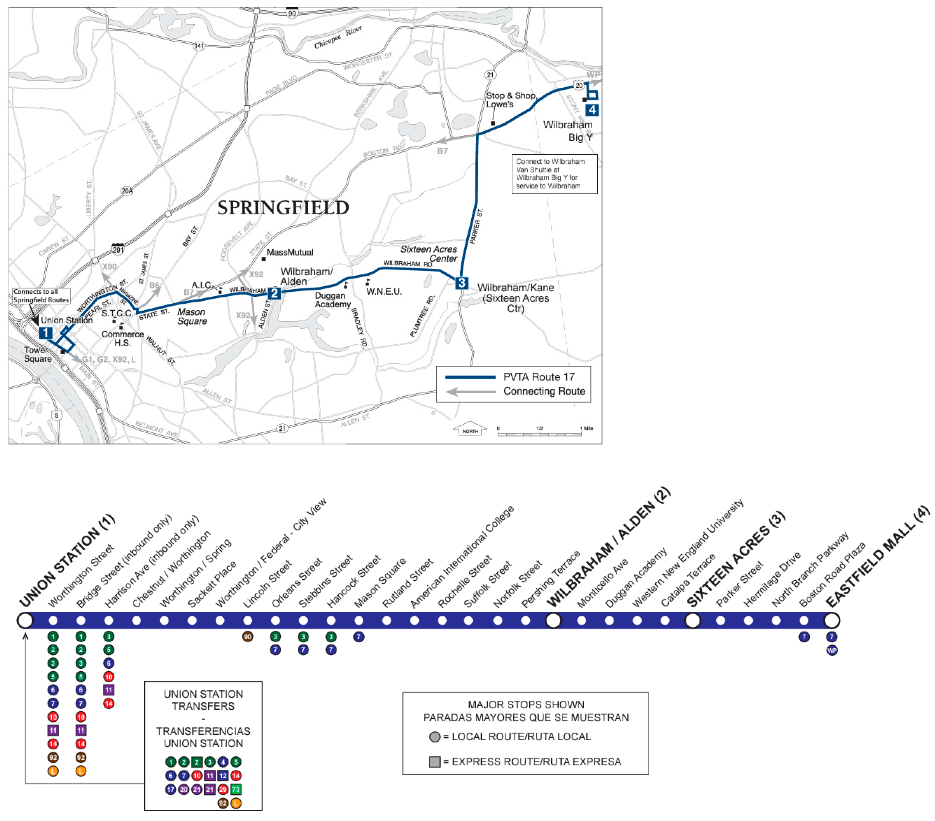Figure 1 illustrates a typical fixed-route bus operation characterized by predefined schedules and fixed stop locations along the travel route.

2. Problem Formulations

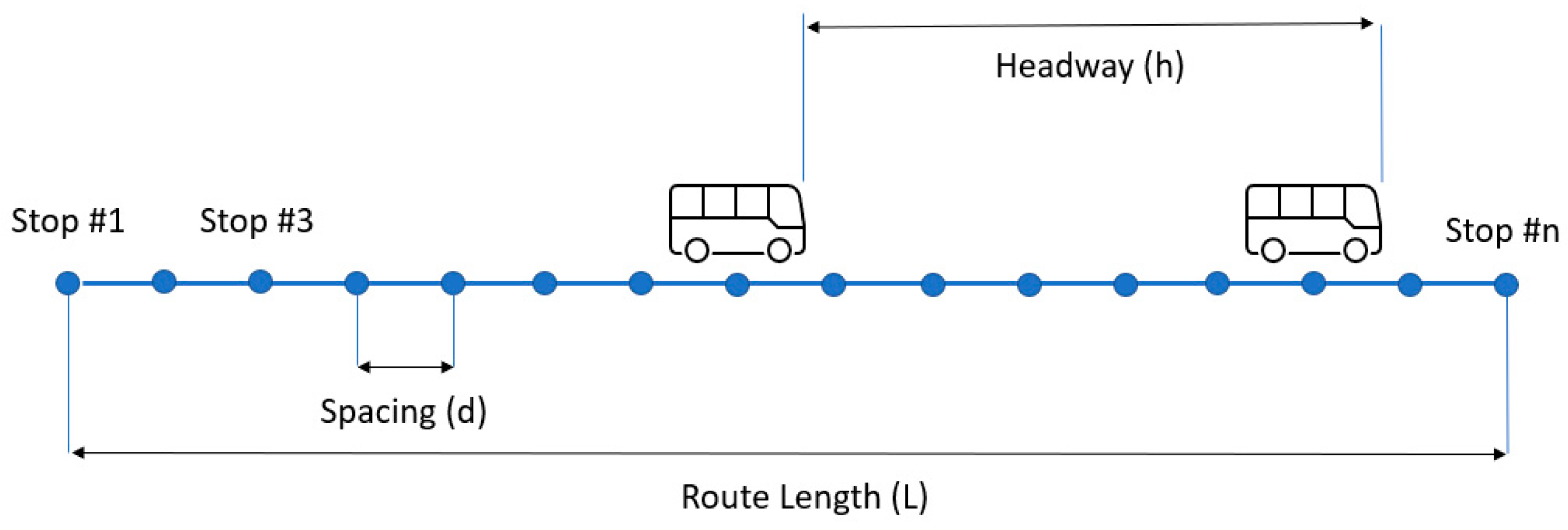
As shown in Figure 2, the bus route has the length of $L$ (in miles) that represents the round-trip distance, and the buses operate with the average speed $V_x$. The bus stops are evenly placed along the bus route. With the bus stop spacing d as an input, the number of stops n along the route is calculated as $L/d$.

As we assume many-to-many demand patterns (i.e., n × n origin/demand pairs), we define the potential demand $q_{ij}$ as the number of potential passengers from bus stop $i$ to bus stop $j$ in passengers/hr. The actual demand $Q_{ij}$ can be estimated based on the elastic demand function in the following section.

2.1. Elastic Demand Function

When addressing minimum cost objectives in transit planning, it is often assumed that demand remains inelastic, unaffected by changes in service quality parameters such as service frequency or fare. However, to relax this strong assumption, so that we formulate bus transit operations with the aim of maximizing profit, it becomes necessary to consider the impact of elasticity on transit demand. Thus, three key elasticity factors that influence actual transit demand are considered. We formulate a linear elastic demand function $k_{ij}$ (from stop $i$ to bus stop $j$) based on the onboard time, waiting time, and fare, as shown in Equation (1)

$$k_{ij}=\left[1-e_w\frac{h}{2}-\frac{e_v}{V_x}\left|j-i\right|d-e_p\left\{\alpha \left|j-i\right|\right\}\right]$$

(1)

where $e_w$ is the demand elasticity parameter for the waiting time, $e_v$ is the demand elasticity parameter for onboard time, and $e_p$ is the demand elasticity parameter for fare based on the onboard distance. Alpha ($\alpha$) is the fare rate in USD/mile.

Then, the actual demand $Q_{ij}$ from stop $i$ to bus stop $j$ is formulated as the product of potential demand $q_{ij}$ and the elastic demand function $k_{ij}$ as follows:

$$Q_{ij}=q_{ij}\left[1-e_w\frac{h}{2}-\frac{e_v}{V_x}\left|j-i\right|d-e_p\left\{\alpha \left|j-i\right|\right\}\right].$$

(2)

It is noted that $k_{ij}$ cannot be negative and is always less than or equal to one. Thus, the actual demand is non-negative and is less than or equal to the potential demand. As shown in Equation (2), the longer waiting time decreases the actual demand, and the increasing onboard time decreases the actual demand. Similarly, increasing fares decrease actual demand.

2.2. Operation Cost

The profit for fixed-route bus transit operations can be calculated by subtracting operation cost from the fare revenue. Thus, we first formulate the cost of bus operations in this section.

The round-trip time $RTT$ is the round-trip distance ($L$) divided by the average bus operation speed $V_x$ as follows. We assume travel distance $L$ is two-way travel distance.

$$RTT=\frac{L}{V_x}$$

(3)

The required fleet size $N$ is obtained by dividing the round-trip time $RTT$ over the headway $h$, as shown in Equation (4).

$$N=\frac{RTT}{h}$$

(4)

The required fleet size $N$ is re-written as:

$$N=\frac{L}{V_{x}h}$$

(5)

The bus operation cost $C_o$ is product of the required fleet size $N$ and the unit operation cost $C_u$. The unit operation cost $C_u$ is formulated based on a fixed cost parameter $a$ and a variable cost parameter $b$ multiplied by the seating capacity $S$. The fixed cost parameter $a$ covers cost components (e.g., labor cost) that are irrelevant to the size of the vehicle. The variable cost parameter $b$ covers other cost components (e.g., maintenance cost) that may vary with the size of vehicles. Therefore, the unit operation cost $C_u$ is formulated as

$$C_u=a+bS$$

(6)

Therefore, the operation cost $C_o$ is obtained by product of required fleet size $N$ and the unit bus operation cost $C_u$.

$$C_o=C_{u}N$$

(7)

The operation cost $C_o$ is rewritten as

$$C_o=\frac{(a+bS)L}{V_{x}h}$$

(8)

It is noted that the operation cost is a function of service frequency. As the bus headway increases, which means less frequent operations, the operation cost decreases.

2.3. Profit

The profit $P$ for bus operations is the amount of revenue $R$ generated by bus services minus the cost of operation $C_o$. The revenue for any origin/destination pair is calculated by the product of distance-based fare and actual demand for the O/D pair. The total revenue from the bus operations is expressed as shown in Equation (9)

$$R={\sum }_i{\sum }_j{f}_{ij}{Q}_{ij}$$

(9)

where f_ij is distance-based fare and $Q_{ij}$ is actual demand from stop i to stop j.

The distance-based fare $f_{ij}$ is proportional to onboard travel distance from stop i to stop j, so it is formulated as

$$f_{ij}=\alpha d\left|j-i\right|$$

(10)

where $\alpha$ is fare rate in USD/mile.

The revenue in Equation (9) is then rewritten as

$$R={\sum }_i{\sum }_j\alpha d\left|j-i\right|Q_{ij}$$

(11)

By substituting $Q_{ij}$ from Equation (2), the revenue is shown as follows.

$$R={\sum }_i{\sum }_j\alpha d\left|j-i\right|q_{ij}\left[1-e_w\frac{h}{2}-\frac{e_v}{V_x}\left|j-i\right|d-e_p\left\{\alpha \left|j-i\right|\right\}\right]$$

(12)

The profit is then calculated by revenue R minus the operation cost C_o, as expressed in Equation (13).

$$P={\sum }_i{\sum }_j\alpha d\left|j-i\right|q_{ij}\left[1-e_w\frac{h}{2}-\frac{e_v}{V_x}\left|j-i\right|d-e_p\left\{\alpha \left|j-i\right|\right\}\right]-\frac{(a+bS)L}{V_{x}h}$$

(13)

The profit function in Equation (13) is the objective function that has two decision variables, namely, the fare rate in USD/mile and the headway in hours. This objective function, shown in Equation (13), has several constraints as follows:

(1)

Elastic demand function $k_{ij}$ for any pairs is greater than or equal to zero and is less than or equal to one. This condition ensures non-negative demand and actual demand is less than potential demand. The number of constraints increases in the order of squares of the number of stops n. (i.e., 2n²). For instance, if n = 10, the number of constraints is 200;

(2)

The optimized headways are always less than or equal to the maximum allowable headway $h_{max}$. This constraint ensures that passengers do not wait for more than one bus, which means that the waiting time for bus is between zero and headway h, resulting in the average waiting time of $h/2$. The maximum allowable headway is calculated as:

$$h_{max}=\frac{Sl}{Q_{max}}$$

(14)

It is noted that maximum sectional demand is based on the actual demand, not potential demand. This is a contribution to literature.

(3)

The profit plus subsidy shall be non-negative. This constraint ensures the operation is financially viable.

3. Solution Methods

3.1. Analytical Solution for Unconstrained Profit Maximization

For the financially unconstrained case, the analytic solution is obtainable. Equation (13), which is the objective function, has two decision variables. As we seek to maximize this profit function, we expect to have a concave curve. Before we derive analytical solutions, we define two substitution parameters $c_1$ and $c_2$ as follows to simplify the expressions:

$$c_1=\sum \sum \left\{\left|i-j\right|q_{ij}\right\}$$

(15)

$$c_2=\sum \sum \left\{{(i-j)}^2{q}_{ij}\right\}$$

(16)

The first order derivative of profit function $P$ with respect to the fare rate $\alpha$ is shown in Equation (17)

$$\frac{\partial P}{\partial \alpha }=d{c}_1-\frac{e_{w}d{c}_{1}h}{2}-\frac{e_v{d}^2{c}_2}{V_x}-2e_{p}d{c}_2\alpha$$

(17)

The first order derivative of profit function $P$ with respect to the headway $h$ is expressed as

$$\frac{\partial P}{\partial h}=-\frac{e_{w}d{c}_1\alpha }{2}-\frac{c_{u}L}{V_x{h}^2}$$

(18)

The second order derivative of profit function $P$ with respect to the fare rate $\alpha$ is as follows.

$$\frac{{\partial }^{2}P}{\partial {\alpha }^2}=-2e_p{\alpha }^{2}d{c}_2$$

(19)

The second order derivative of profit function $P$ with respect to headway $h$ is as follows.

$$\frac{{\partial }^{2}P}{\partial h^2}=-\frac{2c_{u}L}{V_x{h}^3}$$

(20)

As we have a maximum profit objective, we expect the objective function will have a concave curve. Equations (19) and (20) confirm that fare rate $\alpha$ and headway $h$ are the global solutions. To obtain the global solution, Equations (17) and (18) are set to be equal to zero and are solved simultaneously.

3.2. Solution Method for Profit Maximization with Constraints

The decisions we aim to jointly optimize in this study are the fare rate and service headway. It is important to note that the objective function, which seeks to maximize profit, is nonlinear in nature, and the problem formulation encompasses nonlinear constraints. To solve such complex optimization problems (e.g., non-linear mixed-integer optimization problems) effectively, genetic algorithms (GAs) have been used widely [28]. For our solution approach, we have specifically adopted a GA known as real-coded genetic algorithm (RCGA). RCGA utilizes real numbers for encoding, a feature that enables the algorithm to converge to solutions more rapidly compared to other encoding methods such as binary or gray-coded GAs [29,30]. This choice of algorithm enhances the optimization process and facilitates quicker convergence towards optimal solutions.

4. Numerical Analysis

This section discusses the numerical analysis results including sensitivity analyses to the critical input parameters.

4.1. Baseline Results

In this section, we analyze the proposed formulation and its result with the baseline values.

Table 1. Notations and baseline values.

Parameter	Definition	Baseline
$a$	Fixed cost parameter for bus operation in USD/bus-hr	30
$b$	Variable cost parameter for bus operation in USD/seat-hr	0.3
$S$	Vehicle capacity (in seats/bus)	45
$L$	Length of route (in miles)	5
$l$	Load factor (additional vehicle capacity by standees)	1.0
$V_x$	Average bus operation speed (in miles/hour)	40
$d$	Bus stop spacing (in miles)	0.5
$n$	Number of stops (L/d)	-
$I$	Origin counts	-
$J$	Destination counts	-
$e_v$	Elasticity factor for in-vehicle time	0.35
$e_w$	Elasticity factor for waiting time	0.7
$e_p$	Elasticity factor for fare	0.07

shows the baseline input parameters. Other variables are introduced in the formulations.

The potential demand (passengers/hour) for the baseline case is shown in

Table 2. Potential demand matrix.

From/To	1	2	3	4	5	6	7	8	9	10
1	0	10	10	10	10	10	10	10	10	10
2	0	0	10	10	10	10	10	10	10	10
3	0	0	0	10	10	10	10	10	10	10
4	0	0	0	0	10	10	10	10	10	10
5	0	0	0	0	0	10	10	10	10	10
6	0	0	0	0	0	0	10	10	10	10
7	0	0	0	0	0	0	0	10	10	10
8	0	0	0	0	0	0	0	0	10	10
9	0	0	0	0	0	0	0	0	0	10
10	0	0	0	0	0	0	0	0	0	0

. We designed this origin/destination matric as a simple demand structure to explore the demand elasticity as well as sectional demand $Q_i$.

Table 3. Elastic demand factors for O/D pairs.

	1	2	3	4	5	6	7	8	9	10
1	0.980	0.896	0.811	0.727	0.642	0.558	0.474	0.389	0.305	0.220
2	0.896	0.980	0.896	0.811	0.727	0.642	0.558	0.474	0.389	0.305
3	0.811	0.896	0.980	0.896	0.811	0.727	0.642	0.558	0.474	0.389
4	0.727	0.811	0.896	0.980	0.896	0.811	0.727	0.642	0.558	0.474
5	0.642	0.727	0.811	0.896	0.980	0.896	0.811	0.727	0.642	0.558
6	0.558	0.642	0.727	0.811	0.896	0.980	0.896	0.811	0.727	0.642
7	0.474	0.558	0.642	0.727	0.811	0.896	0.980	0.896	0.811	0.727
8	0.389	0.474	0.558	0.642	0.727	0.811	0.896	0.980	0.896	0.811
9	0.305	0.389	0.474	0.558	0.642	0.727	0.811	0.896	0.980	0.896
10	0.220	0.305	0.389	0.474	0.558	0.642	0.727	0.811	0.896	0.980

shows the demand elasticity based on the optimized decisions. We note that as the travel distance increases, the demand elasticity factor decreases. For instance, from stop 1 to stop 2, which is 0.5 miles in distance, the demand elasticity factor is 0.896, which means approximately 10.4% of potential demand is not turned into actual demand. For a case of longer distance travel, from stop 1 to stop 10, the elasticity factor is 0.22 meaning that almost 78% of potential demand is not turned into actual demand. Table 3 also finds that the demand elasticity matrix is diagonal. Additionally, the values of elastic demand factor $k_{ij}$ is between zero and one, as constrained.

The actual demand $Q_{ij}$ is shown in

Table 4. Actual demand matrix.

	1	2	3	4	5	6	7	8	9	10
1	0.00	8.96	8.11	7.27	6.42	5.58	4.74	3.89	3.05	2.20
2	0.00	0.00	8.96	8.11	7.27	6.42	5.58	4.74	3.89	3.05
3	0.00	0.00	0.00	8.96	8.11	7.27	6.42	5.58	4.74	3.89
4	0.00	0.00	0.00	0.00	8.96	8.11	7.27	6.42	5.58	4.74
5	0.00	0.00	0.00	0.00	0.00	8.96	8.11	7.27	6.42	5.58
6	0.00	0.00	0.00	0.00	0.00	0.00	8.96	8.11	7.27	6.42
7	0.00	0.00	0.00	0.00	0.00	0.00	0.00	8.96	8.11	7.27
8	0.00	0.00	0.00	0.00	0.00	0.00	0.00	0.00	8.96	8.11
9	0.00	0.00	0.00	0.00	0.00	0.00	0.00	0.00	0.00	8.96
10	0.00	0.00	0.00	0.00	0.00	0.00	0.00	0.00	0.00	0.00

. We note that the onboard travel distance is a significant factor for passengers to determine whether to use bus operations or not. For instance, when the travel distance is 0.5 miles from stop 1 to stop 2, 8.96 passengers (from 10 potential users) used transit operations. However, when the travel distance is 5 miles from stop 1 to stop 10, the actual demand is only 2.2 passengers per hour from 10 passengers an hour, which is a significant demand reduction. These results confirm that for long-distance travel, transit services with higher speed such as metro rail or bus rapid transit (BRT) should be considered to attract transit ridership.

Table 5. Sectional demand (passengers/hour).

	1	2	3	4	5	6	7	8	9
Q	50.22	89.28	117.18	133.92	139.50	133.92	117.18	89.28	50.22

finds the actual demand along the route, expressed as the sectional demand. $Q_1$ is actual demand between stop 1 and stop 2. Similarly, $Q_9$ is the last section between stop 9 and stop 10. As expected, $Q_5$ shows the highest actual demand along the route, and this maximum sectional demand is used to find the maximum allowable headway.

As the baseline results, the optimized headway is 0.06 h, and the optimized fare rate is 2.27 USD/mile. The revenue generated is USD 2248.69 and the cost of operation is USD 95.10. The maximized profit is USD 2154.15.

4.2. Sensitivity Analysis

In this section, we explore the sensitivity of important parameters to better understand the relationship between policy decisions and modeling outcomes. We analyze four cases: (1) potential demand, (2) fare elasticity factor, (3) average vehicle speed, and (4) unit operation cost.

4.2.1. Potential Demand

For the baseline analysis, we assumed 10 potential passengers per hour for any origin to destination pairs, as shown in Table 2. For the sensitivity analysis, we increased the potential demand from 10 passengers up to 50 passengers with the increment of 10 passengers per hour.

Table 6. Sensitivity analysis results over potential demand (passengers/hour).

	10	20	30	40	50
Headway (hours)	0.06	0.04	0.03	0.02	0.03
Fare rate (USD/mile)	2.27	2.30	2.31	2.31	2.31
Revenue (USD/hour)	2248.69	4553.34	6866.99	9186.21	11,507.93
Cost (USD/hour)	95.10	133.89	163.78	189.68	211.99
Profit (USD/hour)	2154.15	4419.45	6703.21	8996.52	11,295.94

shows the results from the potential demand variations.

In Figure 3, we find that as the potential demand increases, the optimized headway and fare rate appear to remain relatively stable. However, it becomes apparent that both fare revenue and profit values exhibit a nearly proportional relationship with the potential demand. This suggests that as the potential demand grows, fare revenue and overall profit increase accordingly. On the other hand, the operation cost displays a nonlinear relationship, yet it still maintains a degree of proportionality with the potential density. This nonlinearity can be attributed to the fact that actual demand may not exhibit linearly proportional relationships with various cost components.

4.2.2. Fare Elasticity Factor

Table 7. Sensitivity analysis results over fare elasticity factor.

	0.07 (Baseline)	0.14	0.21	0.28	0.35
Headway (hours)	0.06	0.08	0.10	0.12	0.13
Fare rate (USD/mile)	2.27	1.13	0.75	0.56	0.45
Revenue (USD/hour)	2248.69	1104.55	726.30	538.18	426.15
Cost (USD/hour)	95.10	66.63	54.31	46.75	41.84
Profit (USD/hour)	2154.15	1037.92	672.00	491.43	384.30

presents the sensitivity analysis of fare elasticity factor with respect to the system-wide profit. As shown in Figure 4, we observe that the fare rate (a decision variable) displays an inverse relationship with the fare elasticity factor. Notably, as the fare elasticity factor increases, the headway solutions experience a slight increase. This adjustment in headway leads to a reduction in the required fleet size, denoted as N, consequently resulting in decreased operational costs. Figure 5 provides further insights into this relationship. It becomes evident that profit experiences a significant decline as the fare elasticity factor increases. Specifically, profits decrease notably, going from 2154.15 USD/hour with a fare elasticity factor of 0.07 to 384.30 USD/hour with a fare elasticity factor of 0.35. This decline in profit underscores the challenge of maintaining profitability when bus transit operations become more expensive for transit users, highlighting the importance of carefully considering fare policies and their impact on ridership and revenue.

It is worth noting that in our formulation, the fare elasticity factor does not have a significant influence on transit demand.

Table 8. Elastic demand factors for O/D pairs (with fare elasticity factor of 0.35).

	1	2	3	4	5	6	7	8	9	10
1	0.955	0.872	0.790	0.708	0.625	0.543	0.461	0.378	0.296	0.214
2	0.872	0.955	0.872	0.790	0.708	0.625	0.543	0.461	0.378	0.296
3	0.790	0.872	0.955	0.872	0.790	0.708	0.625	0.543	0.461	0.378
4	0.708	0.790	0.872	0.955	0.872	0.790	0.708	0.625	0.543	0.461
5	0.625	0.708	0.790	0.872	0.955	0.872	0.790	0.708	0.625	0.543
6	0.543	0.625	0.708	0.790	0.872	0.955	0.872	0.790	0.708	0.625
7	0.461	0.543	0.625	0.708	0.790	0.872	0.955	0.872	0.790	0.708
8	0.378	0.461	0.543	0.625	0.708	0.790	0.872	0.955	0.872	0.790
9	0.296	0.378	0.461	0.543	0.625	0.708	0.790	0.872	0.955	0.872
10	0.214	0.296	0.378	0.461	0.543	0.625	0.708	0.790	0.872	0.955

presents the results of the elastic demand function with a fare elasticity factor input of 0.35. A comparison with Table 3, which represents the baseline case results, reveals that the actual demand reduction is only 3%. This suggests that changes in the fare elasticity factor have a relatively minor impact on overall transit demand. However, it is important to acknowledge that the fare calculation, based on travel distance, significantly discourages users from opting for bus transit services for long-distance journeys. For instance, the demand reduction from stop 1 to stop 10 registers at 0.214, indicating a substantial 78.6% reduction in actual demand for longer trips. This underscores the sensitivity of passengers to fare increases for extended travel distances.

4.2.3. Average Operation Speed

Furthermore, we conducted a sensitivity analysis to assess how the average speed of bus operations influences transit ridership and profit of the operations. In our baseline scenario, the average vehicle speed is set at 40 mph. When we lowered the average vehicle speed to 10 mph, the demand reduction for passengers traveling from stop 1 to stop 10 amounted to 29%. This outcome confirms the critical role of travel time for passengers when selecting their mode of transportation, particularly for longer-distance trips. The results, as presented in

Table 9. Reduction in actual demand by vehicle speed (from 40 mph to 10 mph).

	1	2	3	4	5	6	7	8	9	10
1	0	3%	4%	5%	6%	8%	11%	14%	20%	29%
2	0	0	3%	4%	5%	6%	8%	11%	14%	20%
3	0	0	0	3%	4%	5%	6%	8%	11%	14%
4	0	0	0	0	3%	4%	5%	6%	8%	11%
5	0	0	0	0	0	3%	4%	5%	6%	8%
6	0	0	0	0	0	0	3%	4%	5%	6%
7	0	0	0	0	0	0	0	3%	4%	5%
8	0	0	0	0	0	0	0	0	3%	4%
9	0	0	0	0	0	0	0	0	0	3%
10	0	0	0	0	0	0	0	0	0	0

, reveal a significant impact on transit demand. It highlights the importance of optimizing bus transit operations to ensure efficient and timely services that attract and retain passengers.

4.2.4. Unit Operation Cost Parameters

For the sensitivity of unit operation cost parameters, we increased these parameters to assess their impact on bus transit operations. Specifically, we raised the fixed cost parameter (a) from the baseline value of 30 USD/bus-hr, increasing it in 10 USD/bus-h increments. Similarly, we raised the variable cost parameter (b) from the baseline value of 0.3 USD/seat-hr, increasing it in 0.2 USD/seat-hr increments. As presented in

Table 10. Sensitivity analysis results on unit operation cost parameters (a and b).

Parameter a
	30 (Baseline)	40	50	60	70
Revenue (USD/hour)	2248.69	2262.92	2254.06	2245.12	2236.81
Cost (USD/hour)	95.10	104.81	114.76	123.19	131.09
Profit (USD/hour)	2154.15	2158.11	2139.29	2121.93	2105.72
Parameter b
	0.3 (Baseline)	0.5	0.7	0.9	1.1
Revenue (USD/hour)	2248.69	2264.17	2142.93	2247.62	2239.82
Cost (USD/hour)	95.10	104.08	112.51	120.61	127.74
Profit (USD/hour)	2154.15	2160.09	2142.93	2127.01	2112.08

, as parameter a or b increases, the cost of operations increases predictably, which aligns with expectations. However, a noteworthy finding is that these unit cost parameters do not significantly influence ridership. Consequently, the reduction in revenue, and subsequently profit, is not substantial in response to these parameter increases. We note that while the optimal fare decision is somewhat related to the cost of operations, the operation cost itself does not have a direct and significant impact on the demand function. If the objective of the problem were to maximize the welfare of bus operations, which considers operator’s profit as well as consumer’s surplus, then the impact of unit operation cost parameters could become more prominent. In such cases, increasing the frequency of bus operations, as explored in studies like Kim and Schonfeld [24], may find that the effect of unit operation cost parameters is more significant.

5. Conclusions

In this paper, we have formulated an optimization problem aimed at maximizing the profit of fixed-route bus operations. We designed an elastic demand function that considers factors such as onboard distance, waiting time, and fare rate. Importantly, our study jointly optimizes headway and fare decisions, with the fare being structured based on the travel distance, rather than using an average fare. The distance-based fare is the fare rate $\left(\alpha \right)$ multiplied by the travel distance (i.e., $\left|j-i\right|d$). We also contributed to the literature by employing actual sectional demand (Q) when calculating the upper boundary of headway (i.e., the maximum allowable headway). The solution to this complex, nonlinear, constrained optimization problem is obtained using a real-coded genetic algorithm. This problem is suitable for one period (e.g., a multiple-hour time block) for a steady demand, and it can be extended to analyze multiple periods to incorporate demand variations along time of day.

Our numerical analyses have confirmed that the proposed solution method finds the optimized fare rate and headway to maximize the profit of fixed-route bus operations. We also found that actual demand for bus transit operations is influenced by various input factors, including fare rate, onboard time, and waiting time. The results in Table 4 and Table 8 show that actual demand tends to decrease as the travel (onboard) distance increases, with a similar pattern observed for extended waiting times for buses. Additionally, as demand density increases, as shown in Table 6, we anticipate more frequent bus operations, resulting in increased profit.

While this work makes significant contributions to the existing literature in public transit planning and operations, there are areas for potential extension and refinement:

(1)

Time variations and additional costs: The proposed formulation is suitable for steady demand within a single period. Extending the analysis to multiple time periods to account for variations in demand throughout the day, and incorporating additional cost components like capital costs, would provide a more comprehensive transit planning model;

(2)

System-wide welfare analysis: Future research can explore the concept of maximizing the net benefit, which combines producer (operator)’s surplus and consumer (passenger)’s surplus, to assess policy changes comprehensively, considering the interests of both service providers and users;

(3)

Fare function enhancement: This paper assumed fares are solely based on travel distance, but the fare structure may be further explored. Additionally, considering a transformation of the distance traveled into an energy consumption metric (e.g., electricity usage) could enable the extension of this study to electric bus operations;

(4)

Elastic demand function: Accessibility can be incorporated into the elastic demand function while the elastic demand function itself can also be improved to reflect the passenger’s model choices. The nonlinear elastic demand function may be explored.

Overall, this presents a useful planning model for fixed-route bus operations, and listed possible extensions can further enhance bus transit planning and operations in public transportation systems.

References

1. Kocur, H.; Hendrickson, C. Design of Local Bus Service with Demand Equilibration. Transp. Sci. 1982, 16, 149–170. [Google Scholar] [CrossRef]
2. Furth, P.G.; Wilson, H.M. Setting Frequencies on Bus Routes: Theory and practice. Transp. Res. Rec. J. Transp. Res. Board 1981, 818, 1–7. [Google Scholar]
3. Zhao, F.; Zeng, X. Optimization of Transit Route Network, Vehicle Headways, and Timetables for Large-scale Transit Networks. Eur. J. Oper. Res. 2008, 186, 841–855. [Google Scholar] [CrossRef]
4. Chang, S.K.; Schonfeld, P. Welfare maximization with financial constraints for bus transit systems. Transp. Res. Rec. 1993, 1395, 48–57. [Google Scholar]
5. Lee, K.K.; Kuo, S.H.F.; Schonfeld, P. Optimal mixed bus fleet for urban operations. Transp. Res. Rec. 1995, 1503, 39–48. [Google Scholar]
6. Kyte, M.; Stanley, K.; Gleason, E. Planning, Implementing, and Evaluating a Timed-Transfer System in Portland, Oregon. Transp. Res. Rec. J. Transp. Res. Board 1982, 877, 23–29. [Google Scholar]
7. Abkowitz, M.; Josef, R.; Tozzi, J.; Driscoll, M.K. Operational Feasibility of Timed Transfer in Transit Systems. J. Transp. Eng. 1987, 113, 168–177. [Google Scholar] [CrossRef]
8. Domschke, W. Schedule Synchronization for Public Transit Networks. OR Spectr. 1989, 11, 17–24. [Google Scholar] [CrossRef]
9. Muller, T.H.J.; Furth, P.G. Transfer Scheduling and Control to Reduce Passenger Waiting Time. Transp. Res. Rec. J. Transp. Res. Board 2009, 2112, 111–118. [Google Scholar] [CrossRef]
10. Lee, K.K.T.; Schonfeld, P. Optimal Slack Time for Timed Transfers at a Transit Terminal. J. Adv. Transp. 1991, 25, 282–308. [Google Scholar] [CrossRef]
11. Chang, S.K.; Schonfeld, P. Optimization models for comparing conventional and subscription bus feeder services. Transp. Sci. 1991, 25, 281–298. [Google Scholar] [CrossRef]
12. Chang, S.K.; Schonfeld, P. Integration of fixed- and flexible-route bus systems. Transp. Res. Rec. 1991, 1308, 51–57. [Google Scholar]
13. Kim, M.; Schonfeld, P. Integrating bus services with mixed fleet. Transp. Res. Part B Methodol. 2013, 55, 227–244. [Google Scholar] [CrossRef]
14. Chandra, S.; Quadrifoglio, L. A model for estimating the optimal cycle length of demand responsive feeder transit services. Transp. Res. Part B Methodol. 2013, 51, 1–16. [Google Scholar] [CrossRef]
15. Nourbakhsh, S.M.; Ouyang, Y. A structured flexible transit system for low demand areas. Transp. Res. Part B 2011, 46, 204–216. [Google Scholar] [CrossRef]
16. Halyal, S.; Mulangi, R.H.; Harsha, M.M. Forecasting public transit passenger demand: With neural networks using APC data. Case Stud. Transp. Policy 2022, 10, 965–975. [Google Scholar] [CrossRef]
17. Pi, X.; Egge, M.; Whitmore, J.; Quin, Z.S. Understanding Transit System Performance Using AVL-APC Data: An Analytics Platform with Case Studies for the Pittsburgh Region. J. Public Transp. 2018, 21, 19–40. [Google Scholar] [CrossRef]
18. Chiang, W.-C.; Russell, R.A.; Urban, T.L. Forecasting ridership for a metropolitan transit authority. Transp. Res. Part A Policy Pract. 2011, 45, 696–705. [Google Scholar] [CrossRef]
19. Berrebi, S.J.; Watkins, K.E.; Laal, J.A. A real-time bus dispatching policy to minimize passenger wait on a high frequency route. Transp. Res. Part B Methodol. 2015, 82, 377–389. [Google Scholar] [CrossRef]
20. Andres, M.; Nair, R. A predictive-control framework to address bus bunching. Transp. Res. Part B Methodol. 2017, 104, 123–148. [Google Scholar] [CrossRef]
21. Chen, L.; Schonfeld, P.; Miller-Hooks, E. Welfare maximization for bus transit systems with timed transfers and financial constraints. J. Adv. Transp. 2016, 50, 421–433. [Google Scholar] [CrossRef]
22. Sun, S.; Szeto, W.Y. Optimal sectional fare and frequency settings for transit networks with elastic demand. Transp. Res. Part B Methodol. 2019, 127, 14–177. [Google Scholar] [CrossRef]
23. McHardy, J.; Reynolds, M.; Trotter, S. A consumer surplus, welfare and profit enhancing strategy for improving urban public transport networks. Reg. Sci. Urban Econ. 2023, 100, 103899. [Google Scholar] [CrossRef]
24. Kim, M.; Schonfeld, P. Maximizing net benefits for conventional and flexible bus services. Transp. Res. Part A Policy Pract. 2015, 80, 116–133. [Google Scholar] [CrossRef]
25. Han, D.; Kim, M.; Kim, E. A planning model for flexible-route bus operation with financial constraint. KSCE J. Civ. Eng. 2022, 26, 3114–3135. [Google Scholar] [CrossRef]
26. Wang, Q.; Schonfeld, P.; Deng, L. Profit maximization model with fare structures and subsidy constraints for urban rail transit. J. Adv. Transp. 2021, 2021, 6659384. [Google Scholar] [CrossRef]
27. Li, Z.-C.; Lam, W.H.K.; Wong, S.C.; Sumalee, A. Design of a rail transit line for profit maximization in a linear transportation corridor. Transp. Res. Part E 2012, 48, 50–70. [Google Scholar] [CrossRef]
28. Goldberg, D.E. Genetic Algorithms in Search, Optimization, and Machine Learning; Addision-Wesley: Reading, MA, USA, 1989. [Google Scholar]
29. Deb, K. An efficient constraint handling method for genetic algorithms. Comput. Methods Appl. Mech. Eng. 2000, 186, 311–338. [Google Scholar] [CrossRef]
30. Deep, K.; Singh, K.P.; Kansal, M.L.; Mohan, C. A real coded genetic algorithm for solving integer and mixed integer optimization problems. Appl. Math. Comput. 2009, 212, 505–518. [Google Scholar] [CrossRef]
Figure 1. PVTA B-17 bus routes (top) and stops (bottom) (in Springfield, MA, USA). Source: www.pvta.com, assessed on 15 March 2023.
Sustainability 15 15352 g001
Figure 2. Fixed-route bus operations (schematic layout).
Sustainability 15 15352 g002
Figure 3. Result variations over the potential Demand (trips/hour).
Sustainability 15 15352 g003
Figure 4. Headway and fare rate result variations over fare elasticity factor.
Sustainability 15 15352 g004
Figure 5. Cost result variations over fare elasticity factor.
Sustainability 15 15352 g005