Abstract
The transport infrastructure sustaining the ascension of land values while synergizing with the industries is a condition optimized for economic sustainability. In general, although transport investment aims to create a more reliable, less congested, better-connected transport network, the secondary aim is to facilitate balanced and sustainable development by enhancing accessibility to infrastructures. Although the current investment principle in Korea more or less reflects the primary purpose, the second aim is not fully reflected and might be too strict about measuring the balanced and sustainable influence on the regional economy. Considering that the house price is an output of regional production, this research tried to establish more proactive quantitative models explaining how ‘transport accessibility to infrastructure’ raises the apartment price in South Korea while interacting with the industries. This study achieved four main results according to the model. First, most urban infrastructures raise apartment prices per square meter about ten times higher than most industries, given a percentage change. Second, the synergy between industrial sales and infrastructural accessibility was negative in most cases, showing a limit of infrastructural investment alone to facilitate sustainable development. Third, an impoverished area tends to conclude positive synergies between industries and infrastructures, justifying more infrastructural investment in those poor areas. Finally, a public service behaves as infrastructure, which re-examines public services’ functionality of the prime water. Conclusively, this research proved that accessibility to core infrastructures is essential in conjunction with land use status resulting from industrial geography to rebalance Korean apartment prices for sustainable investment in transportation sectors.
1. Introduction
Technically, the economic sustainability in transport investment needs something continuous to enhance the economic values of the area invested. One thing more to consider is the economic activity, which the transport investment facilitates, leading to development. After an investment builds a new transport facility to boost economic players in a region, if the representative economic indicator of the region shows continuously positive signs, we can call the investment sustainable, in terms of transportation. Under ultimate sustainability, the average house price should suffer nothing by comparison with the representative economic indicator of a region. Considering that industrial outcomes can affect the region’s economic activity under the same context, finding the triangular mechanism among house prices, industries, and transport leads to the ideal status of sustainable transport from an economic point of view.
Many studies investigated the influence of transport accessibility, industrial sales, or interaction between the two players on house prices. The general economic equilibrium model indicates clearly that transport accessibility interacts with industrial sales to increase house prices. Rothengatter (2017) criticized the current benefit-cost principles for omitting the interactive influence on the whole economic production and suggested combining the interaction and benefit-cost principles [1]. Hensher et al. (2012) proved that the afterward-benefit of the railway construction in Sydney was 17.6% of what the conventional cost-benefit analysis of infrastructure investment calculated. According to the overall steps of the general equilibrium theory, the model adopted by Hensher et al. (2012) calculated the interaction of the accessibility changes due to the railway project with overall industries’ outputs [2]. Furthermore, a house is a product of the regional input-output matrix, and its price includes a result of recursive interaction between transport accessibility and industrial sales or purchases [3].
House prices are one of the critical indicators representing regional economic development, so the factor augmenting house prices raises the regional economic level in the end. Pettinger (2019) concluded that rising house prices generally encourage consumer spending and lead to higher economic growth while falling prices can contribute to the overall economic recession [4]. Using data aggregated per American metropolitan area, Miller et al. (2011) found that an increase in house prices in the USA significantly raised the gross metropolitan product [5]. Commonly recognized, the wealth effect indicates that people spend more as the value of their assets grows [6]. As stated by Cho (2020), house prices in South Korea have also severely influenced its economy, where real estate takes more than 75% of households’ assets on average [7]. The quintile distribution ratio () of the price polarization, 0.899 in 2018, is a social problem initiated by the house price hike in such a short period, exacerbating “the rich-get-richer, the poor-get-poorer”. A national economic problem, housing price polarization, leads the governments to promote national policies to provide 830,000 houses in South Korea [8].
Transportation accessibility enhances economic development by reducing travel time and costs, and thereby some positive effects on housing and other properties can be found. While addressing economic sustainability, we cannot disregard the benefit-cost ratio of the target investment [9]. An increase in the regional GDP notably belongs to the benefit of investments, and the rise in house prices should be a substantial part of the GDP because any regional GDP reflects the recursive interactions among industrial producers in regional input-output production [2]. Therefore, investment in transport and industrial activities create synergies to raise house prices. In Korea, public investments in transport facilities should follow a group of strict principles defining the feasibility test, which deals with direct and indirect economic benefits as the counterpart to the construction costs. The direct benefit represents the travel time saved by the target transport facilities, while the indirect one is the quantitative score decided by the expert group’s qualitative discussion on the regional development effect [10]. The direct benefit, the quantitative part of the principle, has merely focused on linearizing transport networks given time-travel transactions without enough consideration of ‘balancing the economy.’ The indirect benefit links itself to the argument of the contribution to the regional economy from the transport infrastructure’s outputs (accessibility or connectivity) interacting with the regional industries [2,3,11].
Some studies support that transport adjustment can soothe the side effects of house prices. Transportation investment input to the regional economic production causes the price change of general merchandise [3]. In line with Park and Kim (2016), Hensher et al. (2012) explained how the expressway in Sydney increased the regional gross product by combining ‘the traditional benefit-cost analysis of transport investment’ and ‘input-output matrix theory for regional production [2,3]’. Dorantes et al. (2011) investigated how the change in accessibility to urban infrastructures (schools, gyms, parks, or shopping malls) shaped house prices due to the new establishment of the target metro line [11]. Korea’s national transportation investment with a banner of ‘balancing regional development’ also lies in the extension of exacerbating the polarization.
The industries, leading players that contribute to the economic growth in the regional economic equilibrium model, affect house prices, which not a few articles have evidenced. Kim and Jin (2019) found that industrial density measured by accessibility to jobs raised house prices [12]. Wang et al. (2019) indicated that the sum of employment growth multiplied by the number of employees per industry drove up the wages and house prices in China [13]. Zahirovic-Herbert and Gibler (2022) researched Atlanta, Georgia, the south of Hollywood, to establish quantitative models explaining how the film studio restructured the nearby house prices [14]. Interestingly, the houses nearer to film studios recorded lower selling prices, similar to our research result afterward. Moreover, it reveals that the house’s price premium exists if the house near the studio was sold before the establishment of the film studio. This finding shows a difference between the expected price before the development and the actual values after the development. In addition, other studies have already established firm models correlating accessibility with industry positively, which suggests a strong possibility for industries to uplift house prices, as the literature above asserted. OECD (2016) found that the corporate tax growth rate increases as road connectivity rises and that more technological firms get more benefits than otherwise from the connectivities enhanced by the expressways [15]. Lembke and Menon (2016) compared manufacturing and service firms through three hours’ accessibility benefits, where only the service sector recorded a significant marginal effect on productivity growth [16].
There are some studies on the interactions among transport infrastructures and industries, given influences on house prices. Not many pieces of research simultaneously dealt with the influence of ‘transport accessibility and industries’ on house prices. Some studies just researched relations between accessibility and house price, while others did between industries and house prices. Chen et al. (2022) investigated the interactions between connectivity to railway stations and the ‘closeness/betweenness’ of roads given house prices [17]. Their study shows that the closeness of roads interacted with connectivity to railway stations in raising house prices. Zhou and Zhang (2021) investigated the synergies between industrial parks and distances to high-speed railways [18]. In their research, the industry has two categories, manufacturing and service, and it compares four cities in China, which led to contradictory results based on the city’s economic level. Kuklina et al. (2022) researched qualitatively how the tour industry and road developments change Siberia’s economic or social status [19]. Melo et al. (2013) investigated the elasticities of transport infrastructure investment across industrial sectors on the regional GDP, whose structure is similar to our research [20]. Kim and Jin (2019) interpreted the land use index as a representative indicator of the industrial mixture or density but the indicator correlated highly with the house price, the dependent variable [12]. To solve this endogeneity problem, they instrumented the industrial mixture with the connectivity to roads, which contributed to raising the rents of houses. Cho and Choi (2020) found that industries’ interactions with the accessibility to public transport are significantly meaningful in interpreting the Republic of Korea (ROK hereinafter)’s economic structure [21]. Their study captured the extra synergy due to the interactions, which raised the income level aggregated by the municipality district, named ‘Eup’, ‘Myeon,’ and ‘Dong’ in the ROK.
This research aims to recommend concrete pairs of industries and urban infrastructures realizing the positive synergy to raise apartment prices first. Then, it captures the trends penetrating the pairs, which can complete the nation’s regional balanced development policy. This research contributes to the regional development study field by dealing with more industries and accessibility to more diversified urban infrastructures than the incumbent studies. In addition, it analyzed a whole country’s empirical data rather than focusing on several cities so that it produces more insightful and reliable interpretations. Inspired by the clear and concise economic equilibrium theory, this research utilizes multivariate regression models that are simpler and more direct than conventional hedonic models. Moreover, it gives more convenient interpretations of the regression coefficients by adopting logarithmic forms of actual data. Resultantly, this study constructs new principles of designing infrastructures through transport accessibility to facilitate the economic agents, leading to more balanced house prices. The proposals of this research include a way of modifying the principles of infrastructure investment in Korea. This paper not only attempts to examine the interaction between housing prices and transport investments but also tries to identify how to proactively invest in transport infrastructure to stabilize house prices. In this kind of land use and transportation linkage, the housing price reflects premium and can be an economic indicator in measuring the indirect effect of transport investment on housing and property prices.
2. Literature Review
2.1. Sustainability and Land Use Values
Recent studies commonly indicated that maximizing benefits and minimizing costs are indispensable components of economic sustainability [9,22]. Furthermore, continuous economic development is as essential as environmental protection in addressing desirable sustainable infrastructure. According to the International Institute of Sustainable Development (2019), their infrastructure evaluation includes societal and economic benefits such as employment, productivity, income, and GDP contribution [23]. The institution emphasizes that a sustainable infrastructure should facilitate these economic priorities while pursuing the Paris Agreement and UN sustainable development goals. In other words, optimizing economic efficiency in transport infrastructure operations always goes hand in hand with environmental protection. Positively answering these two questions is a baseline condition to minimize the depletion of resources for the infrastructural investment given environmental protection.
Repetitively speaking, a more efficient way inevitably leads to less resource utilization because economic efficiency means minimizing costs using natural resources. Many countries, including Korea, have already adopted this concept in their economic feasibility test for new transport infrastructure. Korea defines the reduced Vehicle Kilometer Travelled multiplied by the unit cost used to treat the CO2 emissions as the quantitative benefits of decreased environmental pollution [10]. The USA, UK, and Japan also regulate their transport facility installation plans based on pollutant emissions, travel patterns, or vehicle types [24].
As Life Cycle Assessment cannot be too crucial regarding economic sustainability [25], the secondary long-term effects of transport infrastructure, such as housing price changes or interaction with industries, are valuable topics to research in constructing the investment principles of transport infrastructure. The first reason is that infrastructure, sustainably augmenting house values, is always welcome by the highest number of regional users. Secondly, if industries, representative regional economic agents contributing to the GDP, produce their wealth in conjunction with the infrastructure, they willingly participate in the infrastructural investment. Needless to say, continuously attracting investors who are willing to pay is the baseline of sustainable transportation, where the investors are the residents and industries.
Transportation facilitates land use, bringing more value by optimizing access to jobs, infrastructures, or markets. However, governments have not considered enough theoretical mechanisms among the factors while investing in transport facilities in general. Kim and Jin (2019) constructed an illustrative mechanism in South Korea, indicating that transport accessibility to jobs raises house prices while mixed-land use drops the indicator [12]. The representative side effect of transport investment could be the polarization in real estate prices, such as residential apartments, which disturbs sustainable investment in transport to a non-negligible degree.
Transportation construction usually contributes to the value of the house and neighborhood properties. Even before the completion of the project, the real estate prices nearby show steep increases due to the expectation. In facing prices soaring or abrupt polarization, Korean governments cannot help hesitating to promote transportation projects. Yiu and Wong (2005) found empirical evidence that a specific railway construction raised the values of Hong Kong’s neighborhood properties before the construction’s completion [22]. Chwidkouski and Zydron (2022) also addressed the significant contributions of the accessibility to bus stops or kindergartens to housing prices in Poznan, Poland [26].
This research further expands the causality, resulting in house prices, to interactions between the accessibilities to infrastructures and industrial sales that have reshaped land use, which previous studies rarely investigated. We assume a causal inference of the target treatment when eliminating the other causal variables’ outcomes [27]. In this research, the treatments are ‘accessibilities’ to urban infrastructures and industrial sales in 2015, and the outcome variable, house price, ranges from 2016 to 2019. In addition, the control variables for eliminating regional effects are more than 200 because this research used cities over 200 in Korea as the control variables. Gray and Lowery (1998) indicates that controlling regions is an effective way to capture unknown variables [28], which OECD (2016), OECD (2017), Lembke and Menon (2016), and Cho and Choi (2020) adopted to increase their explanatory powers [15,16,21,29]. As we have seen so far, several studies support causality among transport accessibility, industrial indicators, house prices, and their interactions. The causality mechanism might be able to stand for a national policy direction to attenuate the house price polarization, which has harassed the Korean governments, by balancing the assets’ values throughout the national territory.
2.2. Methodological Overview
As the introduction indicated, the economic benefit-cost analysis of Korean transportation infrastructure only deals with travel time saving, which the test converts to fiscal value as the quantitative benefit. According to Hensher et al. (2012), the ripple effect comes from the recursive investment of the saved travel time into the regional input-output matrices of which components are the industries [2]. More straightforwardly, enhanced circumstances by the transport investment interact with industries, components of the I-O matrix, to produce a ripple effect that manifests the ‘house prices. Therefore, this research defines the enhanced transport circumstances as better accessibilities to core infrastructures and regards the ripple effects as house prices. Subsequently, the recursive productions through the I-O matrix are equivalent to interactions between the accessibility and the industries’ sales in our regressions.
Multivariate regressions forming hedonic models are famous for addressing apartment prices based on various factors researched. Yiu and Wong (2005) measured the Western Harbor Tunnel construction project’s influences on Hong Kong’s house prices through hedonic regression models utilizing interactions between locations and construction periods [22]. Chwidkouski and Zydron (2022) captured the contribution of infrastructural accessibility on the unit house price through hedonic models [26]. Dorantes et al. (2011) used a hedonic model to assess the circumferential factors’ influences on house price, where apartment amenities, neighborhood characteristics, and transport facilities belong to the factor group considered [11]. Chen et al. (2022) used a hedonic model with interaction between the nearest distance to railway stations and the topological meanings of roads in residential areas to find out their contribution to house prices [17]. Zhou and Zhang (2021) used another hedonic model with the log of the house price as the dependent variable and the interaction between various industries and connectivities to the high-speed railways or city centers [18]. Kim et al. (2016) found that the accessibility to private hospitals (more minor) increased the apartment price considerably while the same indicator of general hospitals decreased the price significantly [30]. Their research’s independent variables contain the structure of the building, interior and exterior features of the architecture, distance to bus, metro stations, and Gangnam area, and accessibility to small, middle, and large-sized hospitals. The variable selection stems from the Hedonic Model, and a multivariate regression model analyzes the microdata. Park and Lee (2012) chose deterioration of the building, brand of apartment, number of buildings in an apartment complex, distance to the firms outstanding in performance, childcare, elementary schools, sports facilities, metro stations, bus stations, firehouse, handicapped welfare centers, and community service center [31]. The dependent variable of Park and Lee (2012) is the unit price of an apartment per square meter, and they used a multivariate regression model to structure the relationship between the independent and dependent variables [31]. Kim and Jin (2019) used ‘conspicuously modified hedonic models’ with a second stage least square method to instrument mixed land use with accessibility to roads or city centers [12]. Their study revealed that industrial density (job accessibility) increased house prices, and mixed land use increased house rents. Wang et al. (2019) used six diversified Hedonic models to address the industrial influences on house prices in China [13]. Zahirovic-Herbert and Gibler (2022) established modified hedonic models to estimate the influence of Atlanta, Georgia’s film industry, on house prices [14]. The OECD publication [29], Cho and Choi (2020)’s research [21], and others using the hedonic model above gave valuable intuitions on advancing the frame of the investigation, structuring a more realistic mechanism between the industry and urban infrastructure.
Those who applied hedonic models typically took the natural logarithm of variables for analytic convenience. Kim et al. (2016), Kim and Jin (2019), Wang et al. (2019), Zahirovic-Herbert and Gibler (2022), and Lembke and Menon (2016) used the natural log of dependent variables [12,13,14,16,30], while Park and Lee (2012) used the natural log of independent variables [31]. OECD (2016) also used logarithmic transformation of the dependent variables, such as firms’ turnovers or wage bills, to capture a percentage change of the input variables, including connectivity or accessibility increases [15].
It is challenging to get all the empirical data to determine the mechanism among house prices, transport accessibility, and industries. Therefore, many studies have adopted semi-empirical or qualitative approaches to address the mechanism. Melo et al. (2013) conducted a meta-analysis using 563 estimated cases extracted from 33 studies [20]. Kuklina et al. (2022) performed in-depth or group interviews with more than 200 individuals to find out the interactions between road access and the tourism industry regarding its contribution to social or economic development [19]. Park and Kim (2016) operated a numerical analysis model to capture the interactive influence on house prices between transport accessibility and industrial sales instead of dealing with empirical data [3].
OECD (2017) [29] adopted the ‘portion of people reaching within specific times’ as the accessibility definition from Tadashi (2013) [32] to investigate the partial correlation between accessibility to public transportation (e.g., bus stops or metro stations) and other socio-economic features. The features included ‘the number of firms per industry,’ ‘population per strata, such as men, women, the elderly, students of different levels,’ and ‘income levels calculated from census data.’ Furthermore, OECD (2017) used the city-level administrative regions as the control variables, eliminating the unique influences that respective cities provided on the output variables [29]. The concept of ‘accessibility’ of OECD (2017) is conveyed to Cho and Choi (2020) [21] who linked ‘accessibility to public transportation with ‘industries or businesses’ to investigate synergies between the two groups.
The advancements of this study distinguished from the previous studies are as follows. First, this research uses actual apartment prices in Korea per square meter instead of the income level, theoretically calculated from housing costs, which Cho and Choi (2020) used [21]. There are no other studies dealing with actual apartment prices in Korea for this type of interactive analysis among accessibility and industries. Secondly, this research applies the portion of the population living in the catchment areas reaching each infrastructure within 15 min by public transportation to the accessibility. This approach gives a more comprehensive concept than Cho and Choi (2020) [21], which used only 10 min of walking distance to bus stations as the accessibility. Thirdly, we used sales instead of ‘the number of industries,’ which Cho and Choi (2020) [21] analyzed, for a more equivalent application to the economic indicator, apartment unit price. The ‘sales’ are more coherent with the general economic equilibrium theory than other indicators such as employment. In addition, more diversified industries appeared to find a more straightforward comparative analysis. Finally, this research investigates all the interactions between ‘accessibilities’ to urban infrastructures and sales of industries for a more detailed and tangible result. General economic equilibrium theory strongly indicates the existence of endogeneity among industries during the process, transforming the regional inputs to output production. Under the same context, many previous studies devised research designs to escape the endogeneity problem when examining industries or accessibility. Our research eliminates this problem from the roots by investigating each pair per regression and excludes most externalities by controlling over 230 variables (cities) from each regression. Consequently, most of the R values of our regressions are over 0.7, which proves the appropriateness of our research design. Practically, the result summarized in Annex gives outstanding policy recommendations to the Korean government about investing in transport for what urban infrastructure and what cities.
3. Data and Method
3.1. Data/Model Framework
This research is not a part of a broader research project, it is a stand-alone study. The research question is “can we find how ‘the accessibility to infrastructure’ and ‘industrial sales’ interact to raise the apartment price?” Before addressing this central question, we need two more questions inspired by ROK’s current feasibility test for new transport infrastructure. The first part of the test concerns the Benefit-Cost ratio, comparing reduced travel time with the construction cost. Because the reduced travel time changes the transportation geography by restructuring accessibility to infrastructure, we assume that the accessibility change reflects the indirect effects of transportation investment after the BC analysis extracted the direct benefit of the reduced travel time at the first stage. Therefore, the second question added for this analysis is, “can we see if accessibility to infrastructure raises the apartment price?” The following third question should be able to measure the influence on the regional economy to check the traditional role of industries in the regional production system. Given that industrial sales could be the main actors comprising regional economy as we reviewed in the previous sections, the question for this part is “Can sales of industries raise the apartment price?”
The first step to solving the second question above is to address the infrastructural influence on the standard price for a residence in Korea. In Korea, locating representative infrastructure such as wide-area railway stations has been susceptible because most Koreans believe that it significantly raises their apartments’ values. Therefore, capturing the quantitative power to level up the asset values sheds light on shaping instructions for urban infrastructural designs.
Secondly, corresponding to the third question above, this study performs a similar procedure to the first step above, using the sales of each industry. The slight difference is taking the natural log of the sales while the previous step uses the natural accessibility, measured as a percentage, to each urban infrastructure. Both steps utilize the natural log of the apartment price per square meter as the dependent variable to capture the percentage change in the price analysis per one percent increase in industrial sales.
Regarding the main research question, the third step investigates the synergy effect by comparing nine combinations per pair of particular infrastructural accessibility and a particular industry. The three representative accessibilities to the infrastructure and three sales of the industry comprise the combinations. We chose the three points based on the U-shaped distribution of the infrastructural accessibility, which gives meaningful testing values with significantly highest, average, or lowest densities. Comprehensively, we can capture principal intuitions on locating urban infrastructure to satisfy the economic agents producing the value-added, nourishing the overall urban economic ecology at this final stage.
For better results, we separate the regional or time effects by adding cities and years as control variables. Our variables are the results of aggregating the raw data by a municipality, of which the number is about 3400. Each municipality belongs to a city, of which the number was about 230 in 2020. Therefore, adding 230 city variables means eliminating every city’s fixed and unique effects (Torress-Reyna, 2007), where the year variables cover 2015 to 2018 [33]. These control variables took a value of ‘1′ if the case belonged to the city or the year. Otherwise, they were zero.
3.2. Data Description
The apartment price per square meter came from the system that provides the apartments’ actual transaction prices from 2015 to 2018. The Ministry of Land, Infrastructure, and Transport operates the actual price database (Ministry of Land, Infrastructure, and Transport) [34]. The total number of actual transactions during the years was several million. We aggregated the prices per municipality (Eup, Myeon, or Dong) and took a natural log form of this aggregated variable in Figure A1b in that the original one showed a highly right-skewed distribution in Appendix B Figure A1a. The curves in Appendix B Figure A1a–c are normal distribution curves estimated. Since the price data are an aggregated form per municipality, extracting the effect of an individual house’s quality or property types is not appropriate. In addition, we control the regional or annual inflation effects by utilizing cities and year variables.
The industries in this research are (A) electronic data management industry, (B) manufacturing industry, (C) wholesale or retail service, (D) transportation industry, (E) lodging or restaurant, (F) public administration service, (G) education service, (H) hygiene or welfare service, (I) institutions or individual services, (J) real estate or rent service, (K) finance or insurance business, (L) construction industry, and (M) science, technology, or professional service. The sales are also right-skewed, so we took the logarithmic form similarly in Figure A1c. When apartment unit price is the outcome variable and an industry’s sale is a predictor, the two’s logarithmic transformation suggests a convenient interpretation. A 1% increase in the predictor leads to the Beta coefficient % of the outcome variable [35]. Moreover, the primary variable’s log transformation meets the linearity assumption more in a multiple-variate regression. According to the general economic equilibrium theory, measuring sales gives a more intuitive result than other indicators, such as revenues. As many universities teach, a row of the input-output matrix represents an industry’s sales to other industries as the intermediate consumptions [36]. The equilibrium theory multiplies the matrix recursively during the equilibrium procedure to determine the price of a product or the change in the price due to a particular industrial sector’s investment increase [3]. Therefore, using sales of industries is natural to find house prices due to transport accessibility changes.
Urban infrastructures used in this research are the target facilities, of which accessibilities the Korea Transport Institute (KOTI) measured officially. The four principal groups of the target facilities are (1) schools (Schools include elementary schools, middle schools, and high schools), (2) clinics (Clinics are public clinics, private hospitals, and general hospitals), (3) markets (Markets are (a) traditional markets, and (b) super-super or mega markets), and (4) metropolitan transport facilities (Metropolitan transport facilities refer to railway stations, metro bus terminals, and airports) [37]. Clinics in our research have public clinics, private hospitals, and general hospitals. A private hospital owns just one or several medical departments, while a general hospital is a complex of overall departments, as the current Korean medical act specifies. Among the transport facilities, KOTI chose only the stations capable of dealing with trains whose delivery capacity was higher than ‘Moo Goong Whoa Ho’ in Korea in the railway domain. The maximum distance reachable within 15 min through the best combination of public transport or walking mode comprises the sole catchment area from the target infrastructure. KOTI carefully performed these calculations with GIS programs, census data, and national facility maps and published the results. KOTI also cautiously selected the target ‘bus terminals’ and ‘railway stations’ according to Korean transport plans defining the functions of those inter-city facilities. In addition, we investigated accessibility in 2015, for which the transport project, the cause of accessibility, had been constructed long before 2015.
In this research, the accessibility to an urban infrastructure took a value from ‘0′ to ‘100,’ measured as the percentage of the population of ‘Eup,’ ‘Myeon,’ ‘Dong’, who can access the infrastructure within 15 min through public transportation modes such as bus, metro, or light train. Interestingly, the accessibility to each urban infrastructure took on a ‘U’ typed distribution, as seen Appendix B Figure A1d.
For readers’ convenience, the third column in Table 1 uses the centered independent variable, subtracting means from the original values so that the mean of the adjusted variable is zero. ‘Ln’ indicates the natural log form of the target variable, and ‘(c)’ does ‘centered.’

Table 1.
Summary of data description.
3.3. Numerical Calculation
The accessibility to each infrastructure is a moderator variable between sales of industry and the unit apartment’s price while addressing and answering the main research question. We assigned the role of interacting to the moderating variable based on the theory of Grace-Martin (2020), which articulates that each interaction variable moderates the other causal or resultant variable [38]. This structure makes it easy to find the most appropriate infrastructure for a specific industry through the lens of contribution to the general economy.
First, this research shapes the design to determine how much each urban infrastructure contributes to the unit apartment price, utilizing Equation (1) below. Equation (1) takes a log of only the dependent variable, where the xi represents the fifteen minutes’ accessibility to ith infrastructure by public transportation. The accessibility adopts the exact definition as OECD (2017) used [29], which was the percentage of persons living in the catchment areas reaching within fifteen minutes among the total population.
Subtracting one from the exponentiating the corresponding parameter of the independent variable gives the percentage change, multiplied by a hundred, in the dependent variable [35]. Equation (2) explains the principle above, mathematically getting the percentage change in the dependent variable.
Secondly, we captured the percentage change in the unit price of the apartment only due to the one percent increase in each industry’s sales. Therefore, the parameter, bi, in Equation (3) indicates the percentage change of the dependent variable, where xi is the sales of the ith industry.
Next, the governing equation corresponding to the main research question is as follows, where and represent accessibility to infrastructure and industry density, respectively. The Equation’s third term, , is the interaction between , ‘accessibility to ith infrastructure,’ and , ‘log of jth industry’s sales.’
To capture percentage changes of the original variables, we transformed the unit apartment price to the natural log form as Y and did the same procedure with ith industry’s sales as xi. The xj in (4) above represents the accessibility to the jth urban infrastructure, expressed as a percentage of people who can reach the infrastructure within fifteen minutes by public transportation. We used xj without the log transformation in that we already scaled its value down from 0 to 100 percent, which can give meaningful differences for comparative analyses. In summary, if a logged ‘sales’ increases by one percent, the logged ‘apartment prices’ increases by the ‘regression coefficient’ percent. However, if the percentage of people with the specified access (the raw independent variable) increases by one percent, the logged ‘apartment prices’ increases by the 100 X‘Exponent of the regression coefficient-1′ percent.
Next, we investigated the marginal effects of the interactions at nine combinations of representative three sales and three accessibilities per pair of industry and infrastructure. For this aim, we chose three accessibilities of the highest frequency, the mean value, and the lowest frequency in the first place. Figure A1d shows the three points of the infrastructural accessibility histogram. This histogram of the accessibility to each urban infrastructure took on a ‘U’ typed distribution that proposes the meaningful points as the highest, lowest frequency, and mean value. Then, we found the ratios of accessibilities chosen to their standard deviation (SD) so that we find corresponding three industrial sales of which the ratios to their SD are the same as the ratios to accessibility’s SD. The three points in the industrial sales and the other three corresponding points in the accessibilities selected based on the accessibility histogram comprise the nine combinations for comparison.
We performed a total of 70 regressions to address the interactions to escape the chronic endogeneity problems while eliminating the other implicit variables’ effects. Under the same context, we performed Equation (1) to capture the percentage change in apartment unit price per infrastructure, as Equation (2) determines. The total number of regressions for Equation (1) was 10 because there are 10 entire infrastructures. As for the industries, we did the regressions 13 times, the number of industries tested, according to Equation (3). The Economic Equilibrium theory regards the endogeneity among industries as natural because it uses the industrial transaction matrix B with the final demands of the industries as the initial input repetitively to produce the total output of the industries [36]. Equation (5) shows the logic.
If there are only two industries in this region, B is two by two square matrix, where Cij means the amount of the ith industry’s goods to produce one unit’s goods of the jth industry. Equation (6) is for reference.
The rationale above proved that the interactive endogeneity among industries would be problematic if we insert several different industries into one regression equation to induce the mechanism between industrial sales and transport accessibility affecting the product (house) price. The house price belongs to the economic equilibrium theory’s total production, so we cautiously performed a regression per target industry and accessibility, excluding the endogeneity and controlling possible implicit variables. The high R values in our results afterward prove that our design is correct.
The next concern is dealing with transport accessibilities to different infrastructures, for which we adopt the strategy of Hensher et al. (2012) [2]. Their research endogenized employment and wages of industries changed by the new railway project in Sydney into the regional economic equilibrium model (Sydney General Economic Model, SGEM). They first calculated changes in trip purpose, transportation mode, travel time, and orientation/destinations. Secondly, the changed pattern produced ‘effective labor density,’ which SGEM utilized as intermediary inputs to its ‘B’ in Equations (5) and (6). Finally, their hybrid model equilibrated the total demands and supplies among the industrial sectors, including ‘Housing sector.’ Therefore, it is worth dealing with accessibility to a specific ‘infrastructure’ and a particular industrial ‘sales’ as separate variables in a regression to see a new horizon addressing transport investment for the infrastructure, given synergy with the specific industry for balancing house prices.
3.4. Limitations
First of all, we could not reach more diversified infrastructures in this study. Those facilities include large-size laboratories for research and development, energy supply complexes, tertiary education classified, leisure or cultural facilities, ports or airports, and others. Considering that some high-tech or entertainment industries need more professional infrastructure than those in this research, we strongly recommend future research dealing with this detailed information. Secondly, the accessibility adopted in this study might usually result from sizable transport infrastructure investments such as road or metro construction but lacks a micro-managed approach such as adjustment of bus transport routing or supplementing public electric scooters. The catchment area, covering 15 min of public transportation, is too wide to deal with the micro-managed transport networks, which reserves further research treating the actual mobility realm in a complicated city.
4. Results and Discussion
4.1. Infrastructural Influence
Table 2 summarizes how much a one percent change in the accessibility to each urban infrastructure contributes to apartment price per square meter. For example, if the portion of persons who can access elementary schools by public transportation in fifteen minutes increases by one percent, the municipalities (e.g., Eup, Myeon, and Dong) experience a 0.683% increase in the average apartment unit price. This resultant number appears at the cross of the second row and fourth column in Table 2. Table 2 summarizes 10 separate regressions: the dependent variable is house price per square meter, and the independent variable is accessibility to each infrastructure while controlling over two hundred and thirty city variables.
Table 2.
Apartment unit price and infrastructure types. ‘***’ indicates the p-value less than 0.001.
4.2. Industrial Influence
Table 3 summarizes how much one percent change in accessibility influences each industry’s sales in percentage. The second column is the percentage increase in the apartment price when the corresponding industry increases sales by one percent. The top industry is the lodging or restaurant business, given raising the residential asset’s unit price. Contrary to common sense, manufacturing lowers the unit price while raising sales by one percent. Table 3 is the summary of 12 regressions: the dependent variable is house price per square meter, and the independent variable is ‘sales’ of each industry while controlling over two hundred city variables.
Table 3.
Apartment unit price and industries. ‘***’ indicates the p-value less than 0.001.
4.3. Interaction Summary
All in all, we have three kinds of interactions: positive, negative, and not significant. Figure 1 illustrates two examples of the interactions, where three lines in different colors are the level of infrastructural accessibility, and three horizontal points are the level of the industry’s sales. Each of the nine points combines the three accessibilities and the corresponding three sales to observe the interaction tendency.
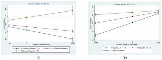
Figure 1.
Comparison between negative and positive interactions. (a) Manufacturing industry and general hospitals, (b) wholesales/retail service and high schools.
A positive interaction makes the apartment price’s growth steeper at higher accessibility to a target infrastructure as ‘sales’ of the target industry increases. If the distance between upper and lower accessibility lines becomes longer as the x-axis’ value increases, the industry and infrastructure conclude a positive interaction, as shown in Figure 1a. If the distance becomes shorter as the sales increase, we see a negative interaction, as shown in Figure 1b. Figure 1a describes interactions between ‘manufacturing’ and ‘accessibility to general hospitals.’ Figure 1b shows the interaction between ‘retail or wholesale service’ and ‘accessibility to high schools.’
We summarize the result of the analyses in Table 4, Table 5 and Table 6 for better visibility. Table 4 gives indices to each industry with upper characters. Table 5 and Table 6 describe the statistical significance and the direction of each interaction between industry and infrastructure. The number of ‘*’ means the level of statistical significance, which the Appendix explains in more detail. ‘+’ is a positive interaction, and ‘-’ is a negative interaction.
Table 4.
Interactions between industries and infrastructures.
Table 5.
Interactions between industries and infrastructures (Index A to G). * indicates the p-value less than 0.05, ** 0.01, *** 0.001.
Table 6.
Interactions between industries and infrastructures (Index H to M). * indicates the p-value less than 0.05, ** 0.01, *** 0.001.
4.4. Discussion
The essence of sustainability is maintaining the target objective’s continuity so that the economic sustainability of transport infrastructure should only keep the society productive economically. Then, how to do that is what this research summarizes. First, investment in transport to enhance the accessibility to urban infrastructure is desirable because the accessibility raises apartment prices per square meter about ten times higher than most industries, given a percentage change. This interpretation compares {Exp(β) − 1} × 100 in Table 2 with β in Table 3. Realizing this instruction makes the investment sustainable because most related residents, hoping for their real estate’s high values, are continuously willing to pay for a new transport facility.
Second, the negative synergy between industrial sales and infrastructural accessibility recommends that we need to reduce direct infrastructural investments in fully developed cities. We observed if there was a synergy between the target variables while excluding externalities by controlling over 230 possible variables, which is a straightforward method, through more than 70 regressions. Therefore, we should utilize different policies to boost such rich regions’ economies by directly enforcing the industrial capacity rather than supplementing transport infrastructures indirectly. Alternatively, as Cho and Choi (2020) indicated [21], we could enhance the accessibility at the minute level, within ten minutes walking distance (e.g., by mobility), not requiring the construction of large-scale infrastructures.
Third, we found that an impoverished area tends to conclude positive synergies between industries and infrastructures, which justifies more infrastructural investment in those poor areas. This valuable takeaway would lead the governments to concentrate selectively on the lagging regions where the synergies with industries are still significant to uplift the real estate’s values. In addition, this strategy is none other than one for sustainable transport to capture the best financial result from limited resources. For example, if we have two billion dollars for a new metro railway project, and if we have to select one region between a sizeable, developed city and a vast underdeveloped region for the project, the lagging region should be the target for a better rate of return. According to this research, if manufacturing firms or public clinics dominate a city, we can regard the city as a lagging region. Korean manufacturing productivity increment rate collapsed from 9.5% from 2000 to 2010 to 2.4% from 2010 to 2017. Korea’s manufacturing competitiveness was lower than the average OECD member by 10% in 2015 [39]. Therefore, we can guess that if house prices are higher than in other regions, the manufacturing firms’ sales decrease because of the increase in fixed costs. In time order, the sales of manufacture were fixed in 2015, after which the market shaped apartment prices. Therefore, we might make a mistake in saying that the decrease in manufacturing sales caused raised house prices. A more appropriate answer might be that manufacturing firms had gathered around poorer places to reduce the fixed cost, after which the geographical condition kept lowering the apartment price. Similarly, the Korean government installed more public clinics in poorer areas to benefit poorer people, after which the geographical conditions of the chosen places continued decreasing the apartment prices.
Finally, the finding that public services behave as infrastructure re-examines public services’ functionality of the prime water to agglomerate people. The water pump needs to be primed with ‘prime water’ to restart the pumping if that pump has not worked for a long time. Public administrative services produce significantly positive synergy with most infrastructures and can do it without financial restrictions that other private sectors should overcome, so they can build a large enough population to activate the agglomeration effect. When the agglomeration reaches a certain level, real estate value rises, as France and China experienced in Combes et al. (2018) and Wang (2016) [40,41]. Similarly, Sejong city, which the Korean government has built as the center of public administration services since 2012, achieved an enormous increase in population by three times in 2020, from 110,000 to 360,000. The government better utilized public services smartly to induce economic sustainability in a new city while providing the new city with transport accessibilities. The interaction of accessibility and industry appears differently according to the region’s development, as this research and Chen et al. (2022) commonly indicate [17]. However, this research newly opens the readers’ eyes to the finding that more developed cities are losing the synergetic power of infrastructures in interacting with industries than those less developed, which suggests a practical and new paradigm of transport investment to balance the regional economic gaps. Furthermore, this research differentiates itself from the previous studies by recommending individual pairs of industry and infrastructure maintaining sustainable power to raise or lower apartment prices, which the government can directly apply to its infrastructural and industrial policy for balanced regional initiatives.
5. Conclusions
The findings are as follows. First, most urban infrastructures raise the unit price of an apartment on average around ten times higher than most industries, in terms of a percentage change. Second, the interactive influence between industrial sales and infrastructural accessibility on the unit price of the house type was negative in most cases, which we can regard as a limit of infrastructural investment alone in facilitating sustainable economic development. Third, a lagging region will likely conclude positive synergies between industries and infrastructures, which supports sizable infrastructure investment in those poor areas. Finally, a public service behaves as infrastructure, which redefines public services’ functionality as the prime water to begin the economy from the bottom.
Limitations of this research, as indicated in Section 3.4, include neither covering the micro-managed accessibility nor professionally diversified infrastructure, which leaves homework to do soon to verify the actual transport function in the sustainable economy to a deeper degree. Comparing this research’s accessibility with a minute level’s accessibility through the lens of principal economic indicators such as income level would be valuable as further research.
Author Contributions
Conceptualization, S.C. and K.C.; methodology, S.C. and Y.Y.; software, S.C.; validation, S.C., K.C. and Y.Y.; formal analysis, S.C.; investigation, S.C., K.C. and Y.Y.; resources, S.C.; data curation, S.C.; writing—original draft preparation, S.C. and Y.Y.; writing—review and editing, S.C., K.C. and Y.Y.; visualization, S.C.; supervision, K.C.; project administration, S.C.; All authors have read and agreed to the published version of the manuscript.
Funding
This research received no external funding.
Institutional Review Board Statement
Not applicable.
Informed Consent Statement
Informed consent was obtained from all subjects involved in the study.
Data Availability Statement
Not applicable.
Conflicts of Interest
The authors declare no conflict of interest.
Appendix A. Each Industry’s Interactions with Infrastructures
For the reader’s convenience, the second column of each industry presents whether the interaction is statistically significant. ‘*’ indicates the p-value less than 0.05, ‘**’ 0.01, ‘***’ 0.001. The third column is the location of checking points, depicted as the ratio of the standard deviation of accessibility to each infrastructure (Ratios to SD for interaction points: Elementary school (−3.361, 0, 0.595); Middle school (−2.2, 0, 0.814); High School (−1.513, 0, 1.052); Public Clinics (−1.094, 0, 1.833); Private Hospital (−2.616, 0, 0.662); General Hospital (−0.727, 0, 1.965); Mega Market (−0.927, 0, 1.512); Traditional Market (−0.927, 0, 1.512); Bus Terminal (−0.542, 0, 3.036); Railway Station (−0.468, 0, 3.389)). Then, we applied the same ratio to SD to an industry’s sales as the accessibility to the infrastructure for investigating the interaction with the industrial sales determined above. Those interaction points below represent the ratio of SD, and all the observations in each industry are 8154.
Table A1.
Electronic data management (SD = 2.027) and Manufacturing industry (SD = 2.729). ** indicates the p-value less than 0.01, *** 0.001.
Table A1.
Electronic data management (SD = 2.027) and Manufacturing industry (SD = 2.729). ** indicates the p-value less than 0.01, *** 0.001.
| Electronic Data | Manufacturing | |||||
|---|---|---|---|---|---|---|
| Interaction Coefficient | Adj. R2 | The Difference in the Base Sales | Interaction Coefficient | Adj. R2 | The Difference in the Base Sales | |
| Elementary School | −0.0004 ** | 0.744 | 0.638 *** | 0.744 | −0.0004 ** | 0.652 *** |
| Middle School | −0.0001 | 0.734 | 0.381 *** | 0.734 | −0.0001 | 0.364 *** |
| High School | −0.0004 *** | 0.73 | 0.27 *** | 0.73 | −0.0004 *** | 0.252 *** |
| Public Clinics | 0.0003 *** | 0.714 | −0.069 *** | 0.714 | 0.0003 *** | −0.072 *** |
| Hospitals (Private) | −0.0002 | 0.750 | 0.562 *** | 0.750 | −0.0002 | 0.572 *** |
| General Hospitals | −0.0002 ** | 0.718 | 0.161 *** | 0.718 | −0.0002 ** | 0.166 *** |
| Mega Market | −0.0004 *** | 0.726 | 0.255 *** | 0.726 | −0.0004 *** | 0.252 *** |
| Traditional Market | −0.0001 | 0.717 | 0.129 *** | 0.717 | −0.0001 | 0.122 *** |
| Bus Terminal | 0.0004 *** | 0.721 | 0.231 *** | 0.721 | 0.0004 *** | 0.253 *** |
| Railway Station | 0.0001 | 0.713 | 0.065 *** | 0.713 | 0.0001 | 0.072 *** |
Table A2.
Retail or wholesale service (SD = 1.907) and Transport industry (SD = 2.079). * indicates the p-value less than 0.05, ** 0.01, *** 0.001.
Table A2.
Retail or wholesale service (SD = 1.907) and Transport industry (SD = 2.079). * indicates the p-value less than 0.05, ** 0.01, *** 0.001.
| Retail or Wholesale Service | Transport Industry | |||||
|---|---|---|---|---|---|---|
| Interaction Coefficient | Adj. R2 | The Difference in the Base Sales | Interaction Coefficient | Adj. R2 | The Difference in the Base Sales | |
| Elementary School | −0.0006 *** | 0.745 | 0.58 *** | −0.0002 * | 0.741 | 0.651 *** |
| Middle School | −0.0004 *** | 0.737 | 0.346 *** | −0.0002 ** | 0.732 | 0.388 *** |
| High School | −0.0009 *** | 0.736 | 0.245 *** | −0.0002 ** | 0.727 | 0.274 *** |
| Public Clinics | 0.0005 *** | 0.719 | −0.078 *** | 0.0003 *** | 0.711 | −0.065 *** |
| Hospitals (Private) | −0.0004 *** | 0.751 | 0.515 *** | −0.0001 | 0.749 | 0.573 *** |
| General Hospitals | −0.0004 *** | 0.722 | 0.158 *** | −0.0001 | 0.715 | 0.168 *** |
| Mega Market | −0.0006 *** | 0.730 | 0.245 *** | −0.0003 *** | 0.724 | 0.264 *** |
| Traditional Market | −0.0003 *** | 0.721 | 0.112 *** | −0.0002 *** | 0.714 | 0.128 *** |
| Bus Terminal | 0.0001 | 0.723 | 0.211 *** | 0.0002 * | 0.717 | 0.238 *** |
| Railway Station | 0.0000 | 0.717 | 0.055 *** | 0.0000 | 0.710 | 0.062 *** |
Table A3.
Lodging or restaurant business (SD = 1.638) and public administrative service (SD = 4.860). ** indicates the p-value less than 0.01, *** 0.001.
Table A3.
Lodging or restaurant business (SD = 1.638) and public administrative service (SD = 4.860). ** indicates the p-value less than 0.01, *** 0.001.
| Lodging or Restaurant Business | Public Administration Service | |||||
|---|---|---|---|---|---|---|
| Interaction Coefficient | Adj. R2 | The Difference in the Base Sales | Interaction Coefficient | Adj. R2 | The Difference in the Base Sales | |
| Elementary School | −0.0008 *** | 0.751 | 0.526 *** | 0.0002 *** | 0.741 | 0.672 *** |
| Middle School | −0.0005 *** | 0.742 | 0.31 *** | 0.0000 | 0.730 | 0.388 *** |
| High School | −0.0009 *** | 0.742 | 0.218 *** | 0.0000 | 0.725 | 0.273 *** |
| Public Clinics | 0.0004 *** | 0.728 | −0.084 *** | 0.0000 | 0.710 | −0.075 *** |
| Hospitals (Private) | −0.0004 *** | 0.755 | 0.487 *** | 0.0001 *** | 0.749 | 0.588 *** |
| General Hospitals | −0.0005 *** | 0.731 | 0.143 *** | 0.0000 | 0.713 | 0.166 *** |
| Mega Market | −0.0008 *** | 0.739 | 0.229 *** | 0.0000 | 0.722 | 0.262 *** |
| Traditional Market | −0.0005 *** | 0.730 | 0.103 *** | 0.0000 | 0.712 | 0.132 *** |
| Bus Terminal | 0.0002 | 0.731 | 0.195 *** | 0.0001 ** | 0.716 | 0.235 *** |
| Railway Station | −0.0001 | 0.726 | 0.052 *** | 0.0000 | 0.709 | 0.07 *** |
Table A4.
Education service (SD = 1.957) and welfare and health service (SD = 1.849). * indicates the p-value less than 0.05, ** 0.01, *** 0.001.
Table A4.
Education service (SD = 1.957) and welfare and health service (SD = 1.849). * indicates the p-value less than 0.05, ** 0.01, *** 0.001.
| Education Service | Welfare and Health Service | |||||
|---|---|---|---|---|---|---|
| Interaction Coefficient | Adj. R2 | The Difference in the Base Sales | Interaction Coefficient | Adj. R2 | The Difference in the Base Sales | |
| Elementary School | 0.0003 *** | 0.745 | 0.632 *** | 0.0004 *** | 0.746 | 0.622 *** |
| Middle School | 0.0001 | 0.736 | 0.342 *** | 0.0000 | 0.737 | 0.314 *** |
| High School | −0.0003 *** | 0.733 | 0.235 *** | −0.0003 *** | 0.735 | 0.209 *** |
| Public Clinics | 0.0001 * | 0.721 | −0.062 *** | 0.0006 *** | 0.728 | −0.103 *** |
| Hospitals (Private) | 0.0001 | 0.751 | 0.545 *** | 0.002 ** | 0.751 | 0.542 *** |
| General Hospitals | −0.0002 *** | 0.724 | 0.15 *** | −0.0005 *** | 0.727 | 0.113 *** |
| Mega Market | −0.0003 *** | 0.732 | 0.248 *** | −0.0006 *** | 0.735 | 0.223 *** |
| Traditional Market | −0.0002 *** | 0.724 | 0.118 *** | −0.0003 *** | 0.726 | 0.073 *** |
| Bus Terminal | −0.0001 | 0.727 | 0.226 *** | 0.0001 | 0.728 | 0.164 *** |
| Railway Station | 0.0001 | 0.720 | 0.074 *** | 0.0000 | 0.725 | 0.037 *** |
Table A5.
Institutions or individual service (SD = 1.593) and real estate rent service (SD = 2.770). * indicates the p-value less than 0.05, ** 0.01, *** 0.001.
Table A5.
Institutions or individual service (SD = 1.593) and real estate rent service (SD = 2.770). * indicates the p-value less than 0.05, ** 0.01, *** 0.001.
| Institutions and Individual Service | Real Estate rent service | |||||
|---|---|---|---|---|---|---|
| Interaction Coefficient | Adj. R2 | The Difference in the Base Sales | Interaction Coefficient | Adj. R2 | The Difference in the Base Sales | |
| Elementary School | −0.0004 ** | 0.746 | 0.552 *** | 0.0002 ** | 0.761 | 0.494 *** |
| Middle School | −0.0004 *** | 0.739 | 0.319 *** | 0.0001 * | 0.756 | 0.268 *** |
| High School | −0.0009 *** | 0.739 | 0.222 ** | −0.0002 *** | 0.755 | 0.184 *** |
| Public Clinics | 0.0005 *** | 0.725 | −0.08 *** | 0.0002 *** | 0.748 | −0.069 *** |
| Hospitals (Private) | −0.0002 * | 0.752 | 0.506 *** | 0.0002 *** | 0.764 | 0.45 *** |
| General Hospitals | −0.0004 *** | 0.727 | 0.144 *** | −0.0004 *** | 0.750 | 0.134 *** |
| Mega Market | −0.0007 *** | 0.735 | 0.235 *** | −0.0004 *** | 0.756 | 0.224 *** |
| Traditional Market | −0.0003 *** | 0.725 | 0.094 *** | −0.0003 *** | 0.750 | 0.082 *** |
| Bus Terminal | 0.0002 | 0.728 | 0.189 *** | 0.000 | 0.750 | 0.157 *** |
| Railway Station | −0.0001 | 0.723 | 0.048 *** | 0.000 | 0.747 | 0.025 *** |
Table A6.
Finance and insurance business (SD = 4.411) and construction industry (SD = 2.240). * indicates the p-value less than 0.05, ** 0.01, *** 0.001.
Table A6.
Finance and insurance business (SD = 4.411) and construction industry (SD = 2.240). * indicates the p-value less than 0.05, ** 0.01, *** 0.001.
| Finance and Insurance Business | Construction Industry | |||||
|---|---|---|---|---|---|---|
| Interaction Coefficient | Adj. R2 | The Difference in the Base Sales | Interaction Coefficient | Adj. R2 | The Difference in the Base Sales | |
| Elementary School | 0.0001 * | 0.745 | 0.604*** | 0.0000 | 0.744 | 0.622 *** |
| Middle School | 0.0000 | 0.736 | 0.309 *** | −0.0002 *** | 0.736 | 0.356 *** |
| High School | −0.0001 ** | 0.733 | 0.209 *** | −0.0002 *** | 0.731 | 0.249 *** |
| Public Clinics | 0.0001 *** | 0.726 | −0.093 *** | 0.0002 ** | 0.718 | −0.066 *** |
| Hospitals (Private) | 0.0002 *** | 0.751 | 0.581 *** | 0.0000 | 0.750 | 0.552 *** |
| General Hospitals | −0.0001 *** | 0.727 | 0.125 *** | −0.0003 *** | 0.722 | 0.153 *** |
| Mega Market | −0.0002 *** | 0.732 | 0.218 *** | −0.0003 *** | 0.729 | 0.244 *** |
| Traditional Market | −0.0002 *** | 0.726 | 0.067 *** | −0.0002 *** | 0.720 | 0.112 *** |
| Bus Terminal | −0.0001 | 0.727 | 0.173 *** | 0.0002 ** | 0.723 | 0.209 *** |
| Railway Station | 0.0000 | 0.724 | 0.024 *** | −0.0002 * | 0.717 | 0.064 *** |
Table A7.
Science, technology, or professional service (SD = 3.660). ** indicates the p-value less than 0.01, *** 0.001.
Table A7.
Science, technology, or professional service (SD = 3.660). ** indicates the p-value less than 0.01, *** 0.001.
| Interaction Coefficient | Adj. R2 | The Difference in the Base Sales | |
|---|---|---|---|
| Elementary School | 0.0001 | 0.750 | 0.553 *** |
| Middle School | 0.0000 | 0.743 | 0.291 *** |
| High School | −0.0001 *** | 0.740 | 0.194 *** |
| Public Clinics | 0.0002 *** | 0.734 | −0.085 *** |
| Hospitals (Private) | 0.0001 ** | 0.754 | 0.502 *** |
| General Hospitals | −0.0002 *** | 0.734 | 0.122*** |
| Mega Market | −0.0003 *** | 0.741 | 0.221 *** |
| Traditional Market | −0.0002 *** | 0.734 | 0.062 *** |
| Bus Terminal | 0.0001 | 0.735 | 0.154 *** |
| Railway Station | 0.0000 | 0.732 | 0.025 *** |
Appendix B. Features of Data

Figure A1.
(a) Original Apartment’s unit price; (b) Log form of apartment’s unit price; (c) Log of Electronic Data Management industry; (d) Accessibility to High Schools by public transportation within 15 min.
Figure A1.
(a) Original Apartment’s unit price; (b) Log form of apartment’s unit price; (c) Log of Electronic Data Management industry; (d) Accessibility to High Schools by public transportation within 15 min.

References
- Rothengatter, W. Wider economic impacts of transport infrastructure investments: Relevant or negligible? Transp. Policy 2017, 59, 124–133. [Google Scholar] [CrossRef]
- Hensher, D.A.; Truong, T.P.; Mulley, C.; Ellison, R. Assessing wider economy impacts of transport infrastructure investment with an illustrative application to the north-west rail link project in Sydney, Australia. J. Transp. Geogr. 2012, 24, 292–305. [Google Scholar] [CrossRef]
- Park, J.H.; Kim, H.B. Impacts of regional accessibility improvement on the national spatial structure. J. Korea Plan. Assoc. 2016, 51, 25–36. [Google Scholar] [CrossRef]
- How the Housing Market Affects the Economy. Available online: https://www.economicshelp.org/blog/21636/housing/how-the-housing-market-affects-the-economy (accessed on 16 February 2020).
- Miller, N.; Peng, L.; Sklaz, M. House prices and economic growth. J. Real Estates Financ. Econ. 2011, 42, 522–541. [Google Scholar] [CrossRef]
- The Wealth Effect. Available online: https://www.investopedia.com/terms/w/wealtheffect.asp (accessed on 17 February 2021).
- Cho, Y.J. Residence Polarization Trend in Korea from 2008 to 2018 through an Actual Survey on Housing; Korean Research Institute for Human Settlement: Sejong, Korea, 2020. [Google Scholar]
- The Public Driven 3080 Policy, Policy Briefing of the Republic of Korea. Available online: https://www.korea.kr/news/pressReleaseView.do?newsId=156435333 (accessed on 19 February 2021).
- Popovic, T.; Kraslawski, A.; Avramenko, Y. Applicability of sustainability indicators to wastewater treatment processes. Comput. Aided Chem. Eng. 2013, 32, 931–936. [Google Scholar]
- Ministry of Land, Infrastructure, and Transport of the Republic of Korea. Direction of Evaluating the Feasibility of Transport Facility Investment; Ministry of Land, Infrastructure, and Transport: Sejong, Korea, 2017. [Google Scholar]
- Dorantes, L.M.; Paez, A.; Vassallo, J.M. Analysis of house prices to assess economic impacts of new public transport infrastructure. Transp. Res. Rec. J. Transp. Res. Board 2011, 2245, 131–139. [Google Scholar] [CrossRef]
- Kim, D.; Jin, J. The effect of land use on housing price and rent: Empirical evidence of job accessibility and mixed land use. Sustainability 2019, 11, 938. [Google Scholar] [CrossRef]
- Wang, J.; Zhu, L.; Li, J. Wages, house prices and industry composition: An empirical analysis of cities in China. J. Asia Pac. Econ. 2019, 24, 618–644. [Google Scholar] [CrossRef]
- Zahirovic-Herbert, V.; Gibler, K.M. The effect of film production studios on housing prices in Atlanta, the Hollywood of the South. Urban Stud. 2022, 59, 771–788. [Google Scholar] [CrossRef]
- O.E.C.D. Road Infrastructure, Inclusive Development, and Transport Safety in Korea; O.E.C.D. Publishing: Paris, France, 2016. [Google Scholar]
- Lembke, A.C.; Menon, C. Impact of Road Infrastructure Investment on Incumbent Firms in Korea; O.E.C.D. Publishing: Paris, France, 2016. [Google Scholar]
- Chen, K.; Lin, H.; Liao, L.; Lu, Y.; Chen, Y.J.; Lin, Z.; Teng, L.; Weng, A.; Fu, T. Nonlinear rail accessibility and road spatial pattern effects on house prices. Sustainability 2022, 14, 4700. [Google Scholar] [CrossRef]
- Zhou, Z.; Zhang, A. High speed rail and industrial developments: Evidence from house prices and city-level GDP in China. Transp. Res. Part A Policy Pract. 2021, 149, 98–113. [Google Scholar] [CrossRef]
- Kuklina, M.; Dirin, D.; Filippova, V.; Savvinova, A.; Trufanov, A.; Krasnoshtanova, N.; Bogdanov, V.; Kobylkin, D.; Fedorova, A.; Itegelova, A.; et al. Transport accessibility and tourism development prospects of indigenous communities of Siberia. Sustainability 2022, 14, 1750. [Google Scholar] [CrossRef]
- Melo, P.C.; Graham, D.J.; Brage-Ardao, R. The productivity of transport infrastructure investment: A meta analysis of empirical evidence. Reg. Sci. Urban Econ. 2013, 43, 695–706. [Google Scholar] [CrossRef]
- Cho, S.; Choi, K. Transport accessibility and economic growth: Implications for sustainable transport infrastructure investments. Int. J. Sustain. Transp. 2021, 15, 641–652. [Google Scholar] [CrossRef]
- Yiu, C.Y.; Wong, S.K. The effects of expected transport improvements on housing prices. Urban Stud. 2005, 42, 113–125. [Google Scholar] [CrossRef]
- The Sustainable Asset Valuation. Available online: http://www.iisd.org/project/SAVi-sustainable-asset-valuation-tool (accessed on 29 April 2022).
- Chung, S.B. Application and estimation of environment pollutant emission considering vehicle driving cycle-focusing on feasibility study. J. Korean Soc. Environ. Eng. 2011, 33, 223–230. [Google Scholar] [CrossRef]
- Six, L.; Velghe, F.; Verstichel, S.; De Meester, S. Sustainability consideration on the valorization of organic waste. In Biotransformation of Agricultural Waste ad By-Products; Elsevier: Amsterdam, The Netherlands, 2016; pp. 287–307. [Google Scholar]
- Chwidkouski, C.; Zydron, A. The impact of urban public transport on residential transaction prices: A case study of Poznan, Poland. Int. J. Geo-Inf. 2022, 11, 1–22. [Google Scholar]
- Green, D.P.; Gerber, A.S. Field experimentation. In Encyclopedia of Social Measurement; Elsevier: Amsterdam, The Netherlands, 2005; pp. 19–24. [Google Scholar]
- Gray, V.; Lowery, D. The Density of State Interest Communities: Do Regional Variables Matter? Publius 1998, 28, 61–79. [Google Scholar] [CrossRef]
- O.E.C.D. Urban Transport Governance and Inclusive Development in Korea; O.E.C.D. Publishing: Paris, France, 2017. [Google Scholar]
- Kim, B.; Ryu, S.; Hong, S. The effect of Medical Service Accessibility on the Housing Price—Focused on Apartment Complex in Gyeonggi-do, Korea. Korea Real Estate Acad. 2016, 66, 188–201. [Google Scholar]
- Park, D.-w.; Lee, J.-H. An Analysis on Impacts of High Tech Complex on Neighborhood Housing price. J. Korea Acad. -Ind. Coop. Soc. 2012, 13, 4543–4550. [Google Scholar]
- Accessibility to Public Transportation: The O.E.C.D. Approach. Available online: https://www.oecd.org/gov/regional-policy/PPT-Transport.pdf (accessed on 3 March 2021).
- Panel Data Analysis Fixed and Random Effects Using STATA. Available online: https://www.princeton.edu/~otorres/Panel101.pdf (accessed on 8 October 2021).
- The System to Open the Actual Transaction Prices of Real Estate (in Korean). Available online: https://rt.molit.go.kr/ (accessed on 30 October 2020).
- Log Log Regression. Available online: https://darrendahly.github.io/post/loglog/ (accessed on 16 February 2021).
- From an Input-Output Table to a General Equilibrium Model: Assessing the Excess Burden of Indirect Taxes of Russia. Available online: http://web.mit.edu/paltsev/www/docs/russia.html (accessed on 17 September 2022).
- Jang, D.I.; Kim, C.S.; Lee, S.J.; Hong, S.P. Establishing Transport Accessibility in Metropolitan Area; The Korea Transport Institute: Sejong, Korea, 2015. [Google Scholar]
- What’s in a Name? Moderation and Interaction, Independent and Predictor Variables. Available online: https://www.theanalysisfactor.com/whats-in-a-name-moderation-and-interaction-independent-and-predictor-variables/ (accessed on 26 November 2020).
- The Falling Competitiveness of the Korean Manufacturing Industry, Falling Short of the OECD Average (in Korean). Available online: https://biz.chosun.com/site/data/html_dir/2019/10/28/2019102800084.html (accessed on 16 June 2021).
- Combes, P.-P.; Duranton, G.; Gobillon, L. The Costs of Agglomeration: House and Land Prices in French Cities. Rev. Econ. Stud. 2018, 86, 1556–1589. [Google Scholar] [CrossRef]
- Wang, A.-M. Agglomeration and simplified housing boom. Urban Stud. 2016, 53, 936–956. [Google Scholar] [CrossRef]

Publisher’s Note: MDPI stays neutral with regard to jurisdictional claims in published maps and institutional affiliations. |
© 2022 by the authors. Licensee MDPI, Basel, Switzerland. This article is an open access article distributed under the terms and conditions of the Creative Commons Attribution (CC BY) license (https://creativecommons.org/licenses/by/4.0/).