Article

An Automated Classification of Recycled Aggregates for the Evaluation of Product Standard Compliance

1
Department of Chemical Engineering, Materials and Environment, Sapienza University of Rome, Via Eudossiana 18, 00184 Rome, Italy
2
Research and Service Center for Sustainable Technological Innovation (Ce.R.S.I.Te.S.), Sapienza University of Rome, 04100 Latina, Italy
3
Centre Terre et Pierre, Chaussée d’Antoing 55, 7500 Tournai, Belgium
4
Höganäs Belgium SA, Ruelle Gros Pierre 10, 7800 Ath, Belgium
*
Author to whom correspondence should be addressed.
Sustainability 2023, 15(20), 15009; https://doi.org/10.3390/su152015009
Submission received: 5 July 2023 / Revised: 13 October 2023 / Accepted: 16 October 2023 / Published: 18 October 2023
(This article belongs to the Special Issue Hyperspectral Imaging for Sustainable Waste Recycling)

Abstract

:
Nowadays, recycling of construction and demolition waste (C&DW) is a challenging opportunity for the management of such end-of-life (EOL) materials through alternative methods to environmentally unsustainable methods (i.e., landfilling). In order to make recycling processes more effective, quality control systems are needed. In this work, the possibility of developing a sensor-based procedure to recognize different demolition waste materials from a recycling perspective was explored. An automatic recognition of different predefined constituent classes of recyclables (i.e., concrete, mortar, natural stones, unbound aggregates, clay masonry units, bituminous materials) and contaminants (i.e., glass, metals, wood, cardboard, and gypsum plaster), as established by an European standard, was carried out using hyperspectral imaging (HSI) working in the short-wave infrared (SWIR) range (1000–2500 nm). The implemented classification strategies, starting from the collected hyperspectral images of the analyzed constituents, allowed for the identification of the different material categories. Two main models were built for identifying contaminants in recyclable materials and categorizing material groups based on technical specifications. The results showed accurate category identification with Sensitivity and Specificity values over 0.9 in all models. The possibility of performing a full detection of C&DW recycling products can dramatically contribute to increasing the quality of the final marketable products and their commercial value, at the same time reducing the amount of waste and the consumption of primary raw materials.

1. Introduction

C&DW represents one of the largest waste streams produced globally. In Europe, about 37% of the total generated waste was represented by C&DW in 2020 [1]. Construction activities, on the other hand, consume large quantities of primary raw materials (i.e., 25% of virgin wood and 40% of gravel and sand annually produced worldwide), resulting in progressive resource depletion [2,3,4].
The fundamental goal to achieve in this context is the optimal management, mitigation, and valorization of C&DW, with particular attention to material recovery. Such a goal is defined by the new circular economy action plan framed in the European Green Deal, since C&DW has been identified as one of the main waste categories of concern for the green transition [5].
C&DW comes not only from the demolition of civil and/or industrial structures, but also from renovation activities or the occurrence of natural calamities (i.e., earthquakes) [6]. In this latter instance, large amounts of rubble are formed in a relatively short period of time, and hence, appropriate handling/processing strategies should be used to free up regions, in order to make structures safe and to perform reconstruction. Those activities are usually associated with further demolition operations, thus producing other C&DW materials to handle [7].
In terms of the characteristics of the originating sources, C&DW is typically composed of many materials (e.g., concrete, bricks, excavated soil, metals, glass, gypsum, wood, plastic, rubber, etc.), characterized by different physical-chemical properties and producing a significant impact on both the setup of efficient recycling strategies and the possibility to generate recovered mono-material flow streams with a low presence of contaminants. This latter aspect is of dramatic importance, since contaminant materials negatively affect the quality of the final products to recycle.
Three primary types of materials providing aggregates, according to existing criteria, can be derived from C&DW: crushed concrete, crushed masonry, and mixed demolition debris to be recycled [8]. Gypsum, metals, plastic, wood, and other pollutants have the potential to weaken the strength of concrete produced with recycled aggregates [9]. Many European countries have established regulations and procedures to encourage the reuse of these materials in road building and in other construction applications, according to their composition and characteristics [10,11,12]. A full classification based on individual constituents (such as concrete, mortar, natural stone, masonry, bituminous materials, glass, metals, wood, plastic, floating materials, etc.) of C&DW in a recycling perspective is thus recommended by legislation in order to define materials suitable for structural concrete [13] or for other applications [14,15].
The possibility of realizing a full separation of materials, also assessing their quality in terms of single recovered flow stream purity (i.e., identification and quantification of contaminants), could represent a big step forward, reducing the dumping of huge quantities of potentially reusable and/or recyclable materials [16,17,18]. The adoption of processing strategies able not only to separate the materials, but also to verify their quality in a simple, robust, reliable, and cost-effective way is necessary in order to reach this goal. Moreover, the economic aspect is of paramount importance mainly for two reasons:
  • The relatively low values of the materials that are potentially recoverable from C&DW flow streams. The development of low-cost processes is thus linked to the production of large quantities of material per time unit, which must also be of high quality;
  • The dimensions of the enterprises involved in this business. Usually, in fact, they are of small or medium size, and normally, they want to perform the job as quickly and as cheaply as possible, utilizing simple technologies and thus causing an important loss of recoverable materials and a corresponding reduction in revenues [19].
Starting from these premises, the only possibility for performing better C&DW recycling is through the increase of recovered product quantity and quality, the utilization of simple technologies, and an increased market consciousness versus a larger material recovery.
To achieve the latter goal, various processing perspectives, based on C&DW constituent material maximization recovery, must be adopted. Plastics and/or wood, or milled brick flow streams, for example, have thus been regarded as resources to be recovered rather than contaminants within recycled aggregates. Additionally, innovative and low-cost analytical tools capable of performing continuous and comprehensive monitoring of the various generated C&DW-based flow streams must be developed, implemented, set up, and fully utilized.
The fulfillment of the previously mentioned targets represents the only way to fight and cut down some of the actual existing barriers related to the utilization of recycled aggregates, such as (i) a low quantity of C&DW-derived products; (ii) a not-clear perception in the market of the advantages, both in environmental and economic terms, linked to the utilization of more specific and focused C&DW processing practices; and (iii) a legislation that does not favor their use, etc. All these facts negatively interact with each other, thus enhancing the suspicion associated with the use of recycled C&DW products.
In the last decade, different studies were carried out to explore the possibilities offered by novel mechanical recycling systems and procedures to obtain high-grade recycled aggregates [18,19,20,21]. To provide one example, the European C2CA project looked into a combination of smart demolition, grinding crushed concrete in an autogenous mill to improve the liberation of cement mortar from the surface of aggregates, and a unique dry classifying technique called Advanced Dry Recovery (ADR) to remove the smaller particles [18]. Gebremariam et al. [20] discussed the development of the Heating-Air classification System (HAS) together with the ADR. These industrial-scale technologies are designed to recycle end-of-life (EOL) concrete into coarse, fine, and ultrafine particles. Therefore, ADR serves the purpose of separating clean coarse aggregates, whereas the HAS is employed to create pristine fine aggregates through the heating and separation of the ultrafine hydrated cement constituents. Moreover, in order to create a more environmentally friendly and sustainable system, Ferrández et al. [21] suggested adding two new steps of processing, demonstrating that they dramatically lower the impurity content and water absorption of recycled aggregates, resulting in a superior end product (cement mortar) for constructions.
In this perspective, this work aimed to show the possibilities offered by an innovative optical sensing technology aided by machine learning to improve and to speed up C&DW recycling in the characterization, sorting, and quality control stages. In more detail, the developed approach is based on hyperspectral imaging (HSI). This technology could successfully contribute to filling the existing gap between C&DW recovered products and their full characterization and certification.
An HSI procedure in the short-wave infraRed (SWIR) range (1000–2500 nm) was implemented to detect recyclables (i.e., concrete, mortar, natural stones, unbound aggregates, clay masonry units, and bituminous materials) and contaminants (i.e., glass, metals, wood, cardboard, and gypsum plaster) as defined by the European standard EN 933-11:2009 [22]. SWIR-HSI enables the identification of different materials on a properly energized sample surface based on their reflectance spectra [23,24], according to the presence of specific chemical bonds (i.e., O-H, N-H, C-H, S-H, …) that are obviously linked to their composition. The HSI technique allows for the acquisition, collection, and management of spectra of a properly energized surface sample [23,24]. The collected spatial and spectral information is arranged in a 3D dataset, the so-called hypercube, characterized by two spatial dimensions and one spectral dimension. Starting from the information constituting the “hypercube”, material characteristics and assessment, in the investigated flow stream, can be thus determined. Spectral features are linked to samples’ physical-chemical attributes, thus allowing for full sample characterization, classification, and quality control.
In the last few years, HSI has become more prevalent in the solid waste industry, and its use in the DW recycling sector has begun to take hold [25,26,27,28].
HSI-based techniques are cost-effective, reliable, simple to apply, and easy to implement both at the stationary and mobile plant scales. An HSI-based approach can allow for the continuous monitoring of C&DW-derived products, which can result in the subsequent certification of the processed materials.

2. Materials and Methods

2.1. Selected Samples

The Federation of Recycling Construction Waste (FEREDECO) in Wallonia (Belgium) provided mixed demolition waste samples to the Centre Terre et Pierre (CTP, Tournai, Belgium), a certified research center, which performed tests at a pilot plant scale in order to simulate a separation line for inert materials from C&DW. A first screening step was carried out to remove the finest particles (−15.00 mm) and the particles with a size of +15.00 mm were then crushed. A new screening step was then carried out on +15.00 mm particles, and three size classes were obtained (i.e., +60 mm, −60.00 +30.00 mm, and −30.00 mm classes). Crushed particles with a size of −30 mm were then wet-sieved to remove the −4.00 mm fraction, which was too fine to be visually characterized. The −30 mm +4.00 mm fraction was then immersed in water and slightly stirred to separate floating from sinking particles.
The floating materials (i.e., autoclaved aerated concrete particles), constituting the Fl category, were recovered and dried. The sinking materials were dried in a ventilated oven at 60° for 24 h, and then they were classified into the six categories defined by the European standard EN 933-11:2009 [22], which are as follows:
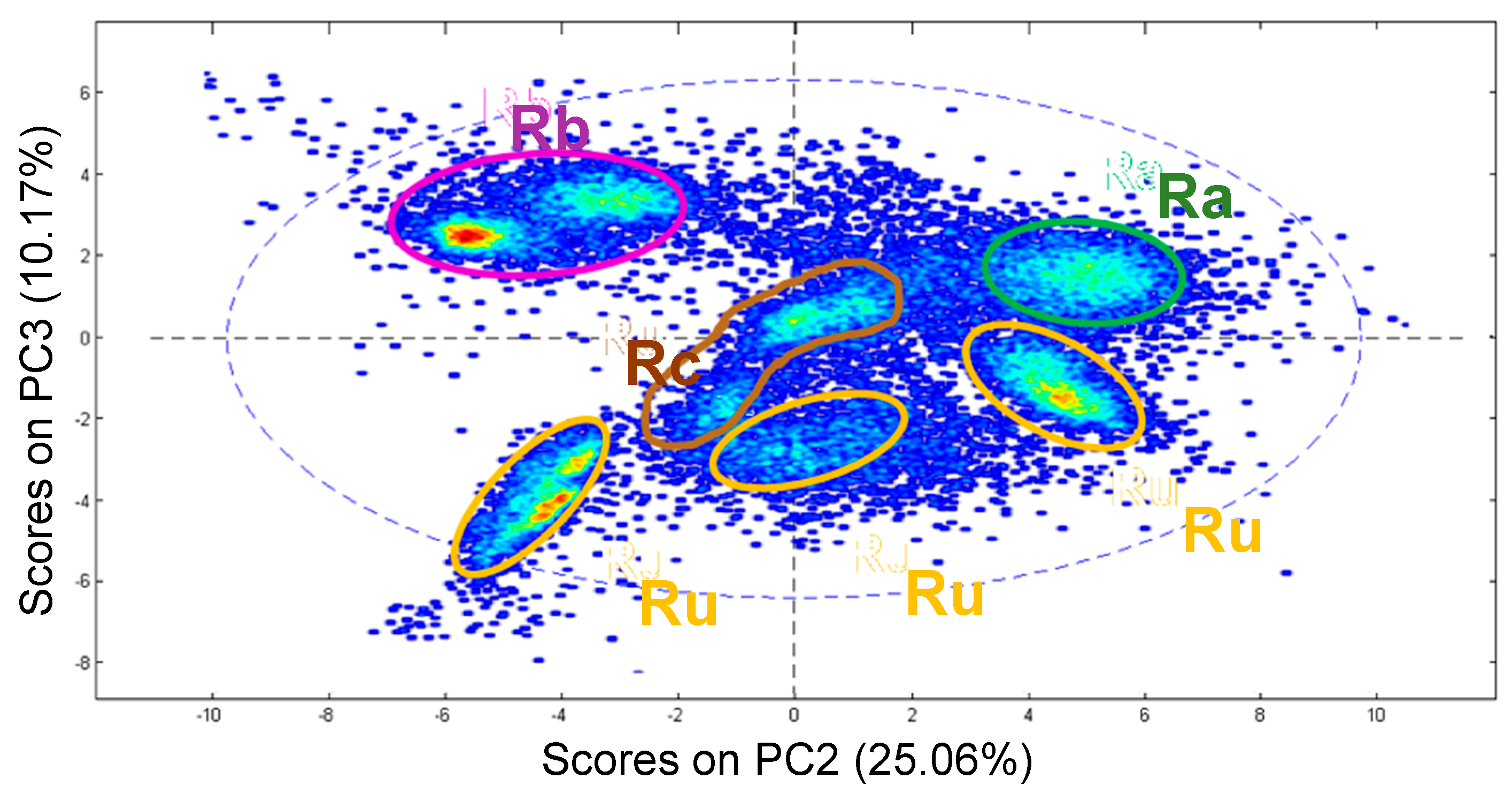
  • Rc: Concrete, concrete products, mortar, and concrete masonry units;
  • Ru: Unbound aggregates, natural stones, and hydraulically bound aggregates;
  • Rb: Clay masonry units (i.e., brick and tiles), calcium silicate masonry units, and aerated non-floating concrete;
  • Ra: Bituminous materials;
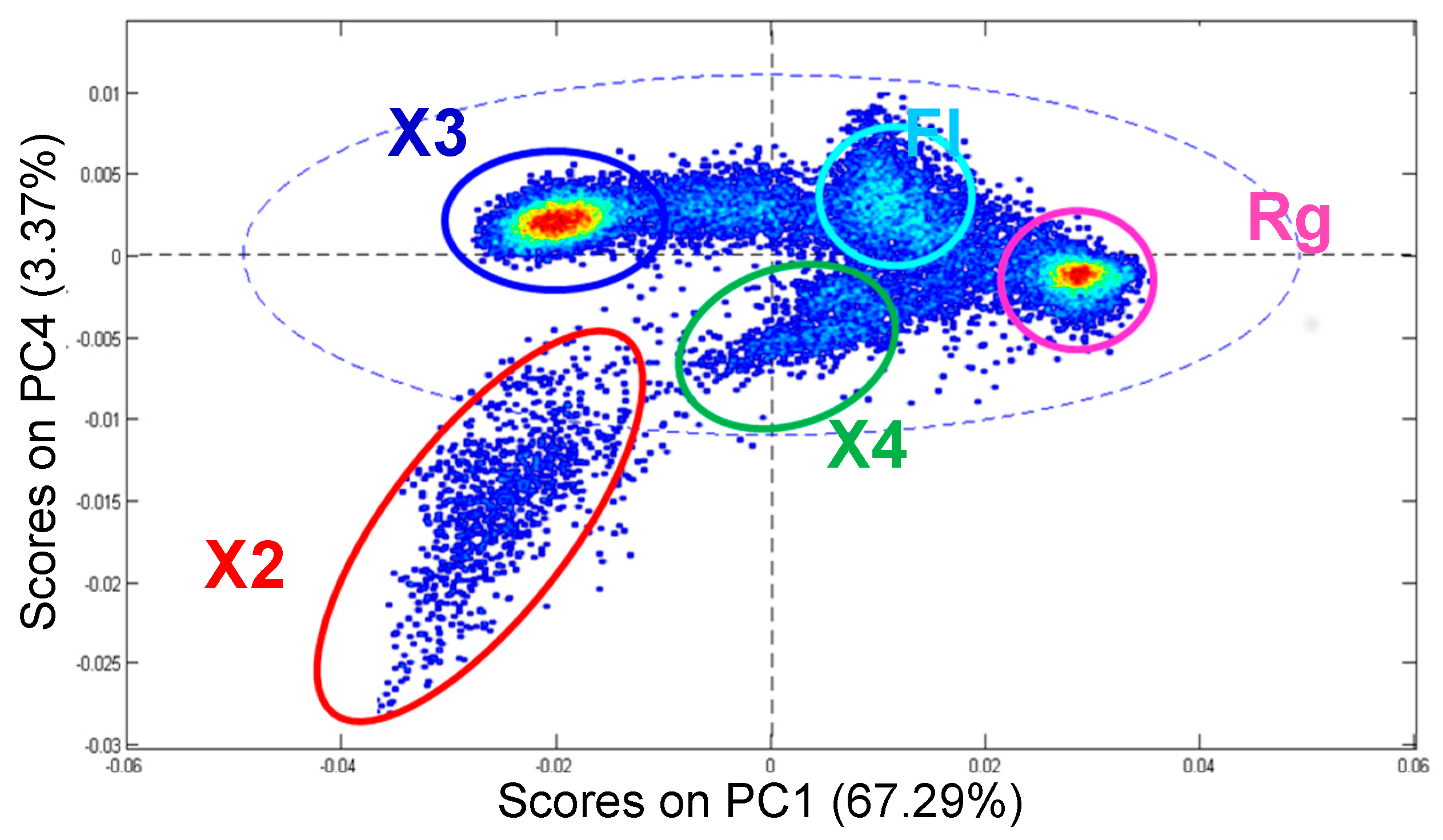
  • Rg: Glass;
  • X: Other cohesive materials (i.e., clay and soil) and miscellaneous materials, such as metals (ferrous and non-ferrous metals), non-floating wood, plastic and rubber, and gypsum plaster.
Class X was then subdivided into four classes:
  • X1: Metals (ferrous and non-ferrous);
  • X2: Non-floating wood;
  • X3: Cardboard;
  • X4: Parget and gypsum plaster.
The categories Rc, Ru, Rb, and Ra were considered recyclable materials in accordance with the legislation, while classes Fl, Rg, X1, X2, X3, and X4 were considered contaminants with respect to the main applications of C&DW products (i.e., road foundations, material production as aggregates for concrete, etc.).
The list of the 10 different categories of materials is summarized in Table 1.
From each of the 10 categories, particles were selected, and HSI-based classifications were performed, adopting two different acquisition set-ups as described in the following:
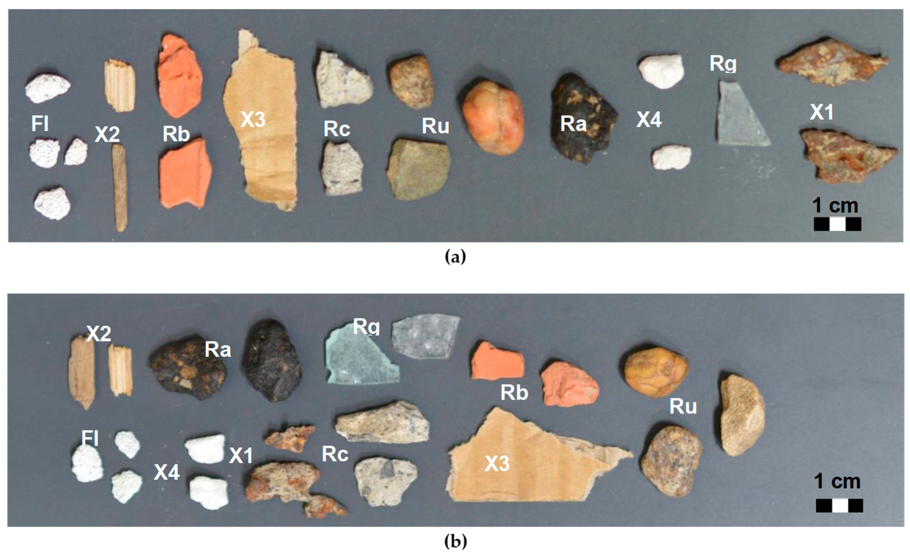
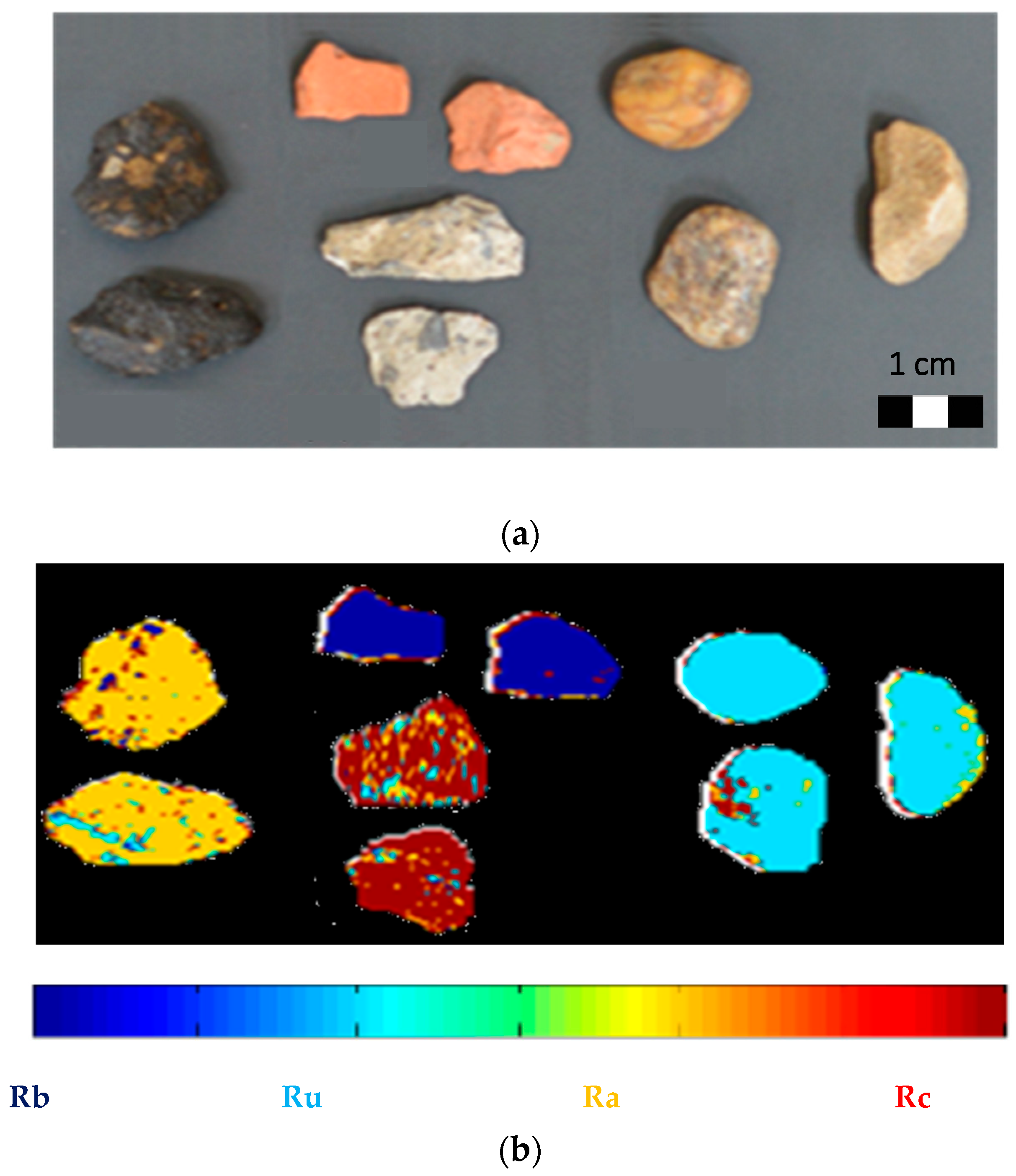
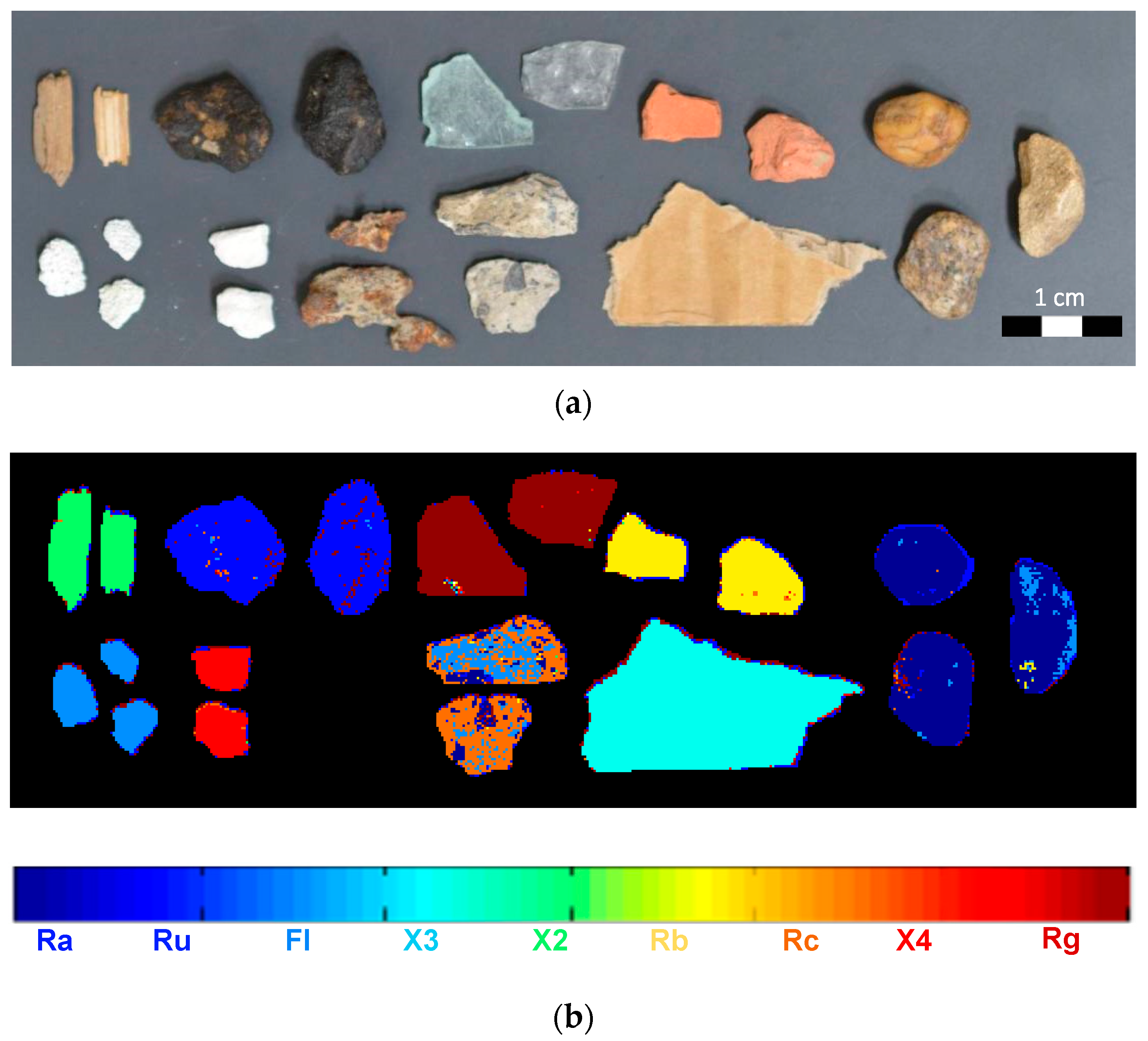
  • 1st set-up. A training image to be utilized for the classification stage was generated (Figure 1a). More specifically, a set of 20 particles clearly identified as floating materials (4 particles), wood (2 particles), masonry (2 particles), paperboard (1 particle), concrete (2 particles), aggregates (3 particles), hydrocarbons (1 particle), parget (2 particles), glass (1 particle), and metals (2 particles) were used in order to build the classification model.
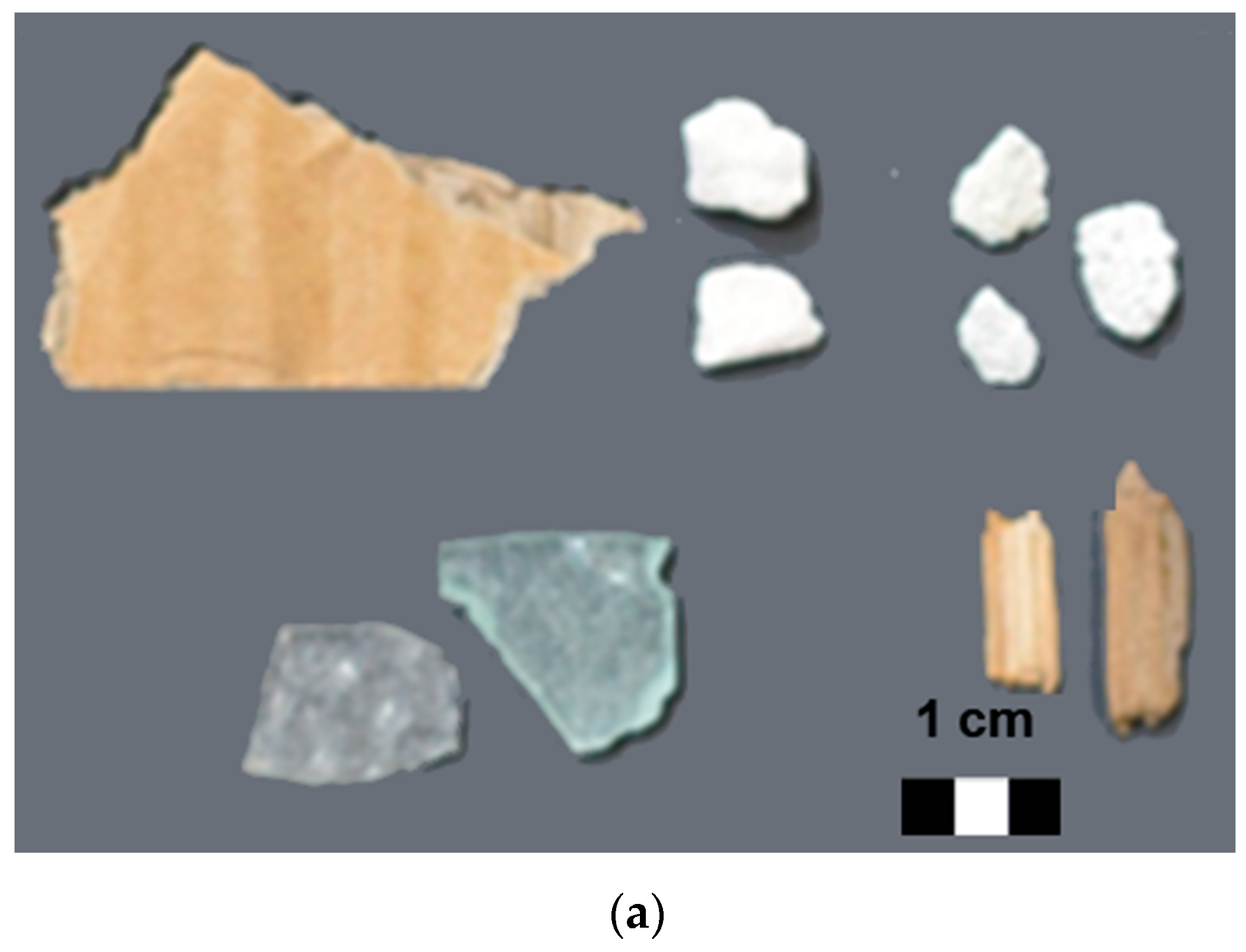
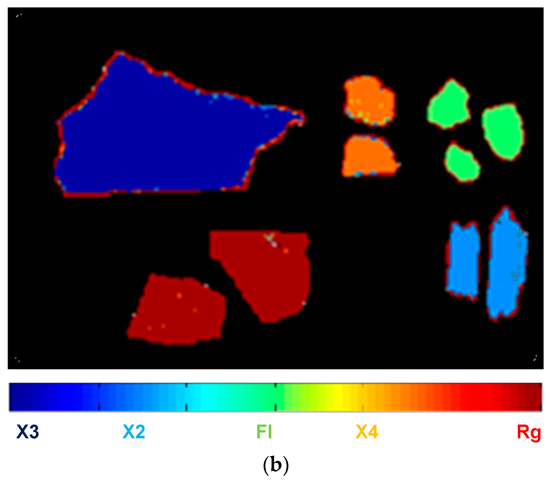
  • 2nd set-up. A validation image, constituted by particles of the same materials but different from those utilized for training, was then created to perform the validation (Figure 1b).

2.2. Hyperspectral Imaging System

Hyperspectral imaging acquisitions were carried out at the Raw Materials Laboratory (RawMaLab) of the Department of Chemical Engineering, Materials and Environment (Sapienza—University of Rome, Rome, Italy).
The analyses were performed in a controlled environment, imitating the operative conditions of a similar sensing unit in a real processing plant. However, the push-broom acquisition logic of the HSI system (e.g., the sensor remains stationary while the object being observed is moved) simulates a conveyor belt setup that can be employed in a processing facility.
A SisuCHEMA XL Chemical Imaging Workstation (Specim Spectral Imaging Oy Ltd., Oulu, Finland), equipped with an ImSpector N25E imaging spectrograph (Specim Spectral Imaging Oy Ltd., Oulu, Finland) and working in the SWIR range (1000–2500 nm), was used. More in detail, a 31 mm lens with a field of view of 100 mm was adopted, and 256 wavelengths were collected. To acquire, collect, and manage hyperspectral data, ChemaDAQ software (Ver. 3.62; Specim Spectral Imaging Oy Ltd., Oulu, Finland) was used. Spectral data were analyzed using PLS_Toolbox (Ver. 8.2; Eigenvector Research, Inc., Wenatchee, WA, USA) and MIA_Toolbox (Ver. 3.1.0; Eigenvector Research, Inc., Wenatchee, WA, USA) working in a MATLAB (Ver. 8.6; The Mathworks, Inc., Natick, MA, USA) environment.

2.3. The Developed HSI Procedures

Starting from the same training data set, two different strategies were adopted in order to discriminate Rc, Ru, Rb, Ra, Fl, Rg, X1, X2, X3, and X4, as described in the following:
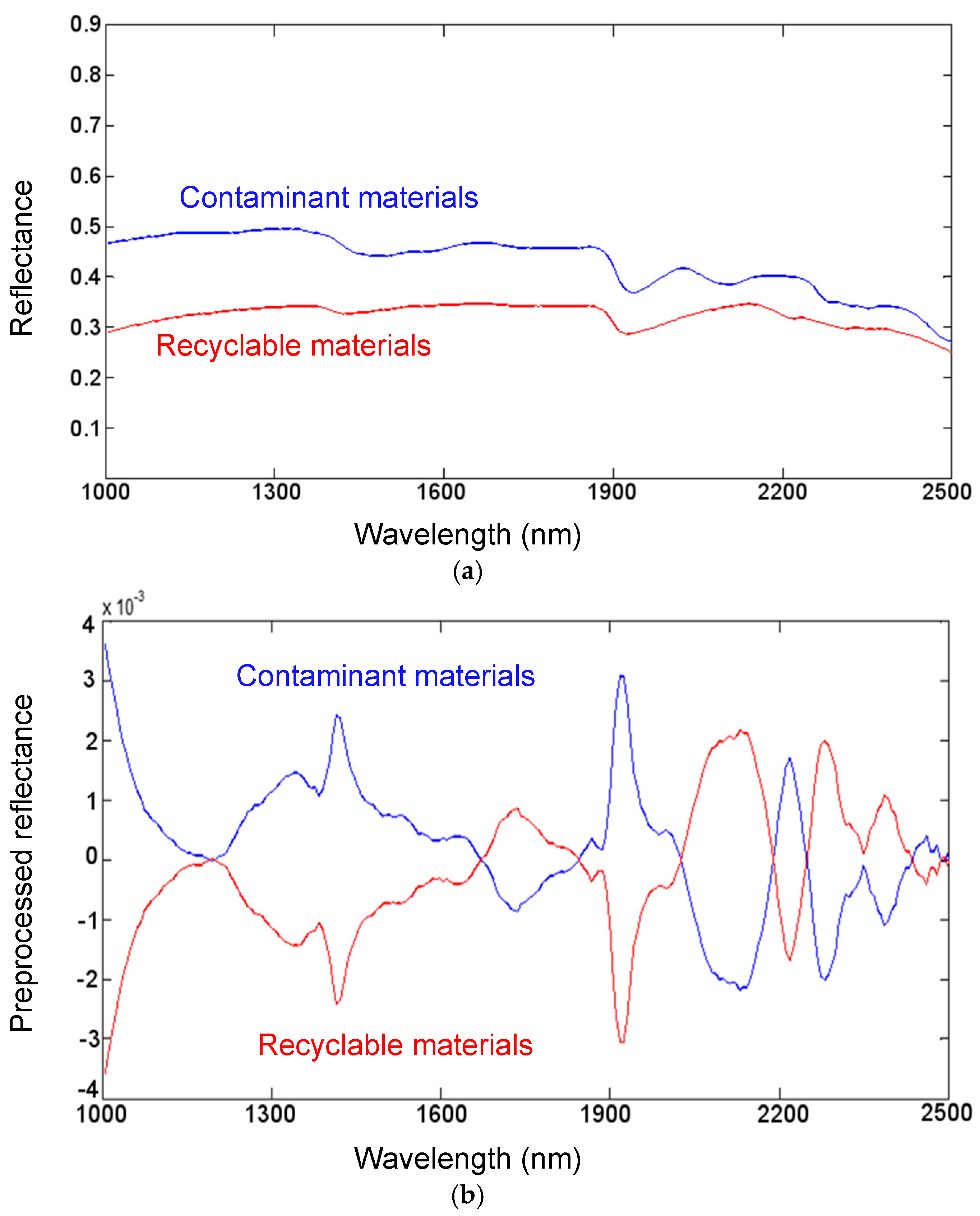
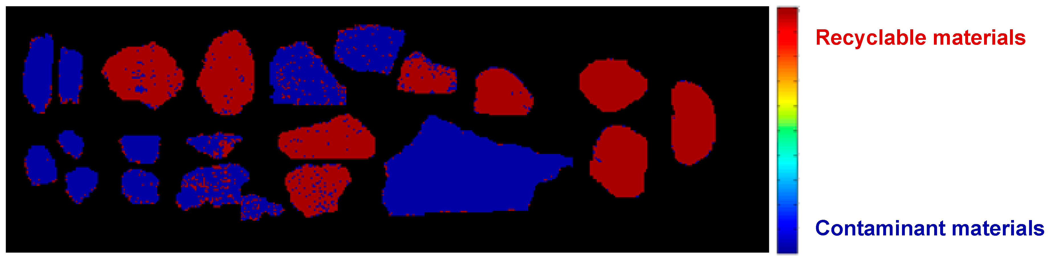
  • Two-classes model. In the first strategy, a two-classes model was built to identify recyclable (Class 1: Rc, Ru, Rb, and Ra) and contaminant (Class 2: Fl, Rg, X1, X2, X3, and X4) materials. Two classification models were then developed to recognize the single materials of Class 1 (4-classes model) and of Class 2 (5-classes model), assuming that the X1 class was removed during a metal removal step (i.e., magnetic separation).
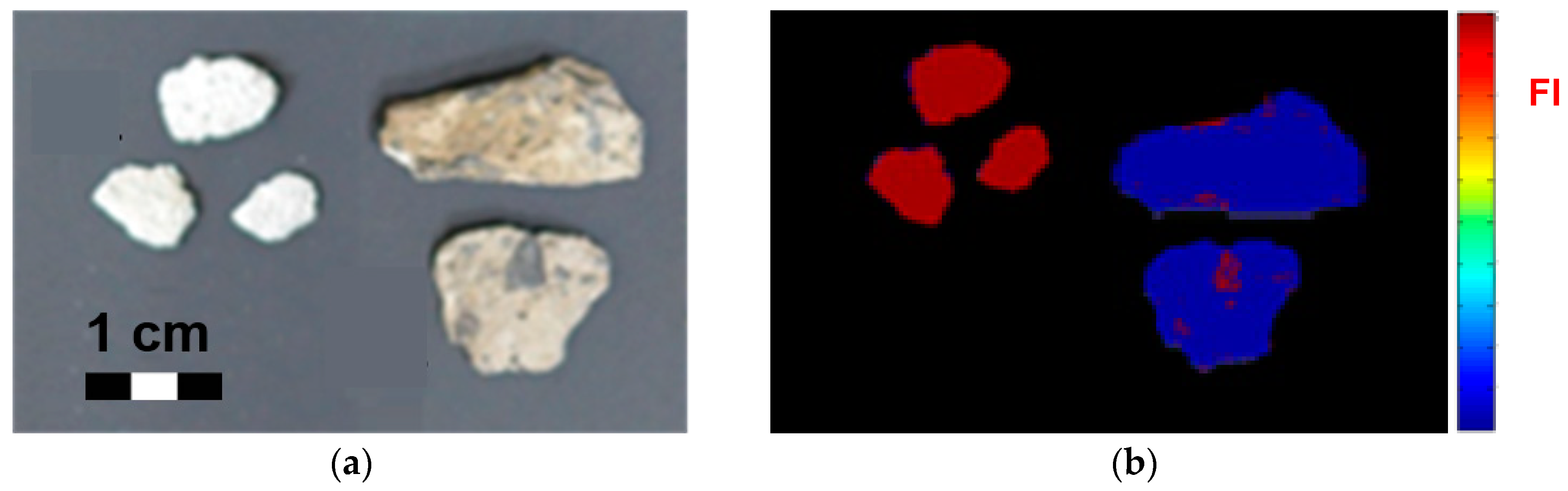
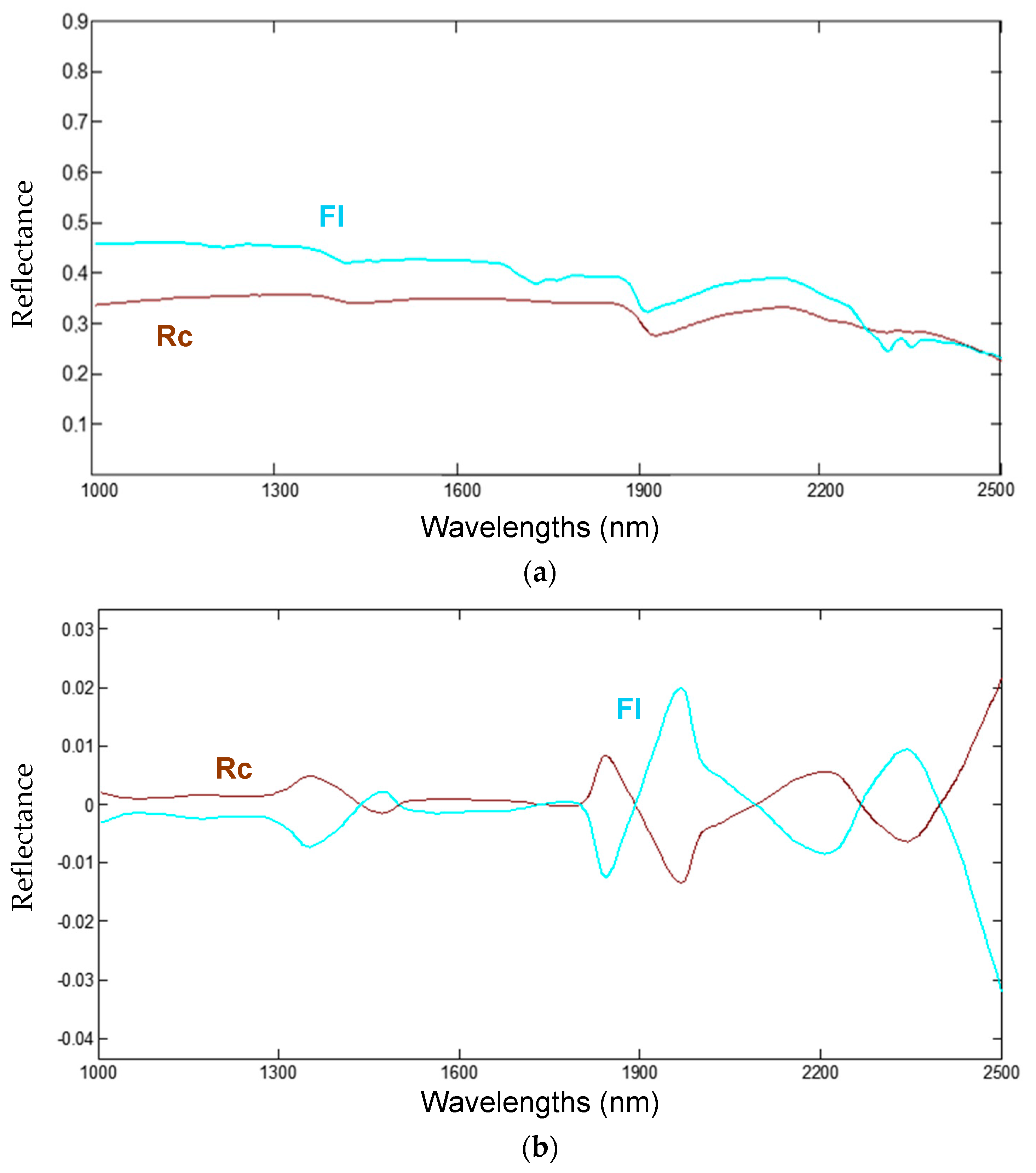
  • Nine-classes model. In the second strategy, a metal removal step (i.e., magnetic separation of X1) was firstly assumed, and then the remaining 9 categories of materials (i.e., Rc, Ru, Rb, Ra, Fl, Rg, X2, X3, and X4) were classified individually by a single model. Since Rc (i.e., concrete) is sometimes misclassified with Fl (i.e., floating materials/autoclaved aerated concrete), a 2-classes model to discriminate only these two concrete categories was built.
Starting from the 2nd set-up, for each classification purpose, a subset of particles was picked up and arranged in order to build the corresponding validation dataset.
A simplified scheme showing the adopted procedures is reported in Figure 2.
For the 2-classes model (i.e., “recyclable materials” and “contaminant materials”) classification strategy, due to the huge variability of spectra, regions of interest (ROIs) were selected on the training image in order to set the classes to be recognized in the validation image. In the other cases, a training dataset for the following classification purposes was obtained by selecting pixels belonging to each different investigated category based on principal component analysis (PCA) score plot. Spectra preprocessing was applied in each experimental setup in order to highlight the differences between the considered classes. Preprocessed spectra extracted from ROIs or PCA scores clusters were used to train the partial least-squares–discriminant analysis (PLS-DA) classification models. Classifications and model validations were finally defined using test sets.

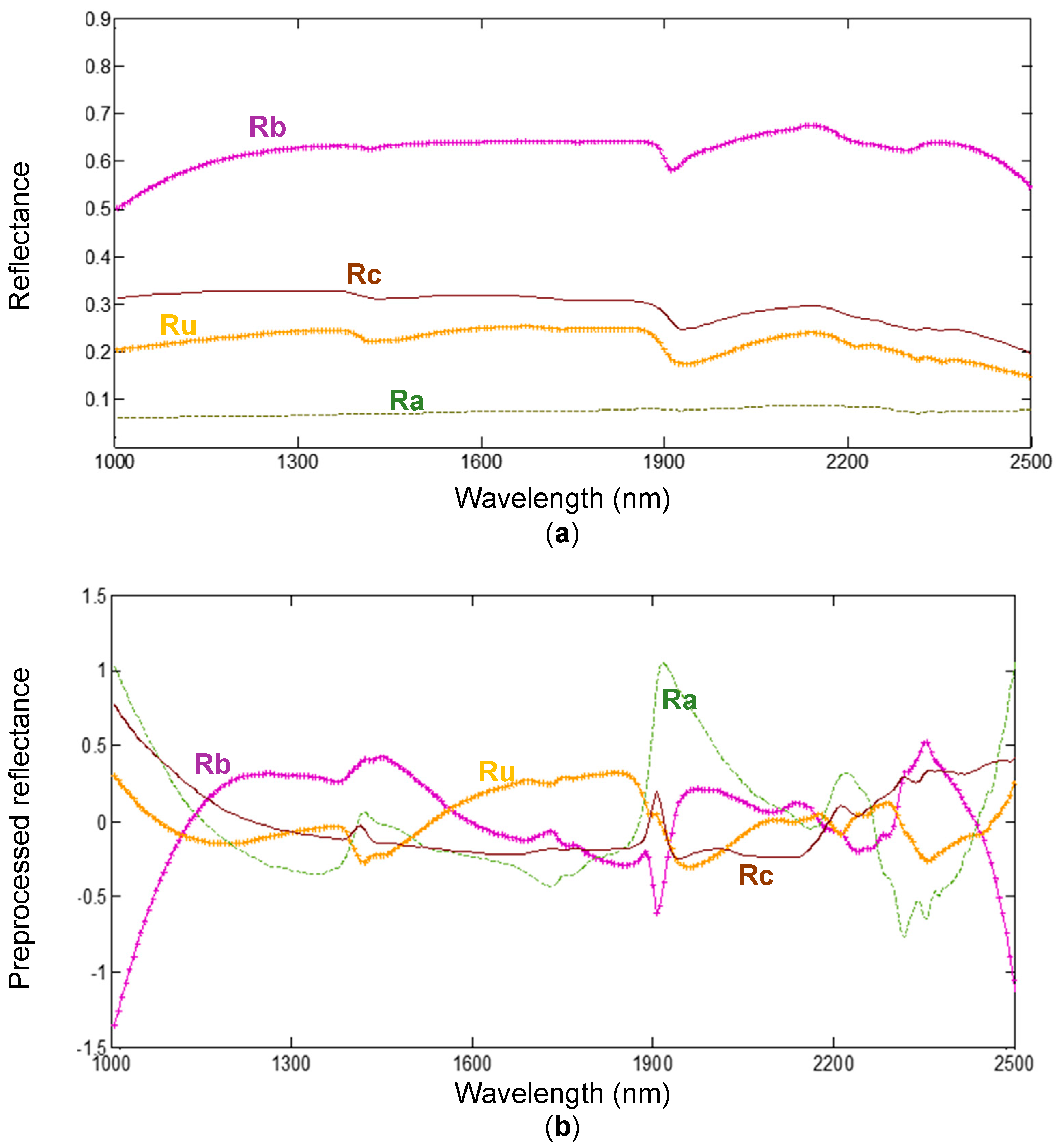
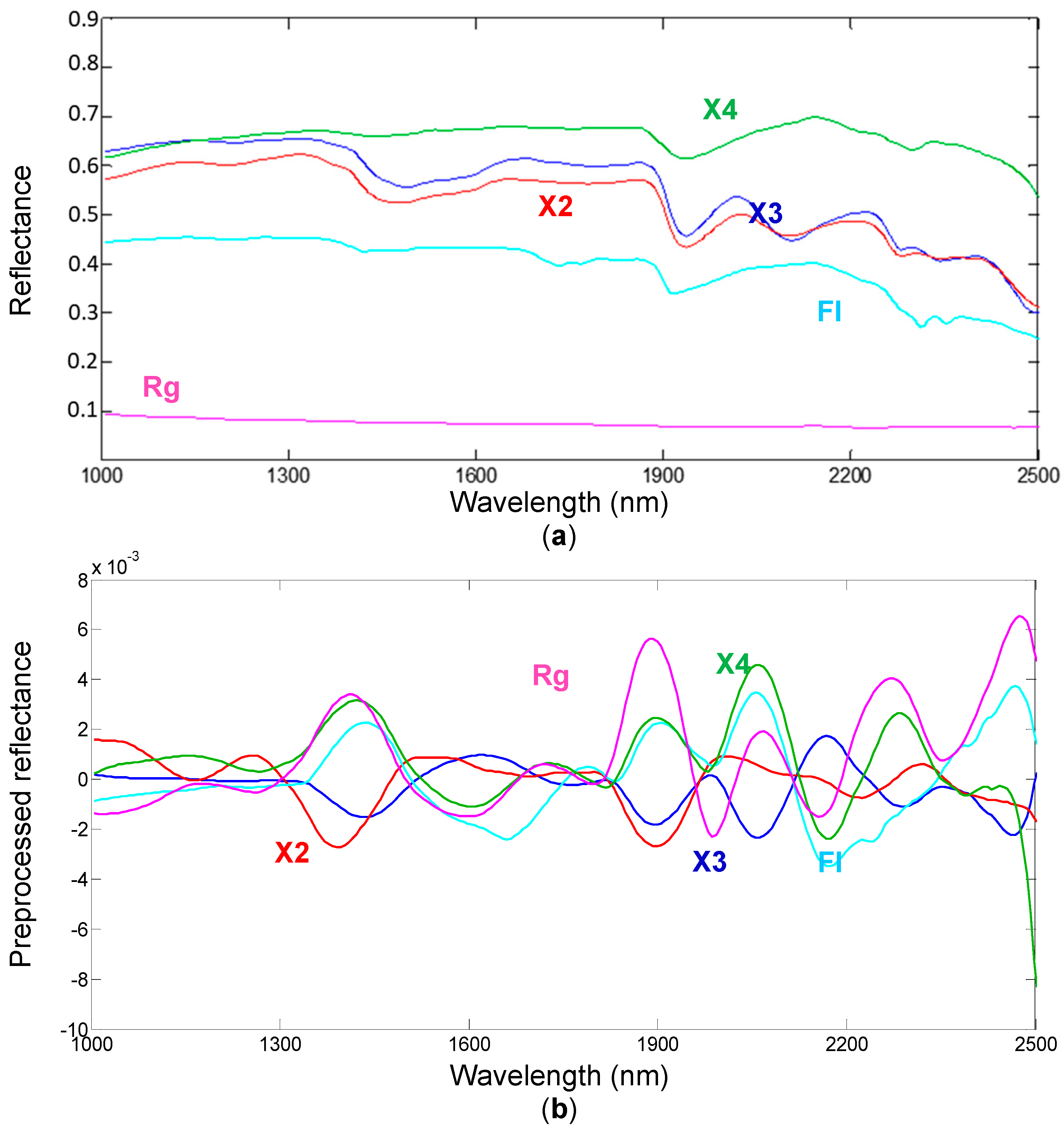
2.3.1. Spectra Preprocessing

Spectral data were preprocessed to enhance sample spectral features and to reduce the impact of possible external sources of variability [29]. Preprocessing was carried out utilizing the sequential application of different algorithms such as mean center (MC), Savitzky–Golay derivative, detrend, standard normal variate (SNV), and generalized least-squares weighting (GLSW).
MC is one of the most common preprocessing methods, and it is useful to remove constant offsets not significant for the data variance interpretation [30]. Derivative is a useful method for removing baseline signal from samples, the detrend algorithm was applied to remove constant, linear, or curved offset, while SNV is a weighted normalization used to solve scaling or gain effects, due to path length effects, scattering effects, source or detector variations, or other general instrumental sensitivity effects [31]. The GLSW algorithm calculates a filter matrix based on the differences between pairs or groups of samples that should be similar [32]. The filter matrix aims to reduce the weight of these variations, which are regarded as interferences.

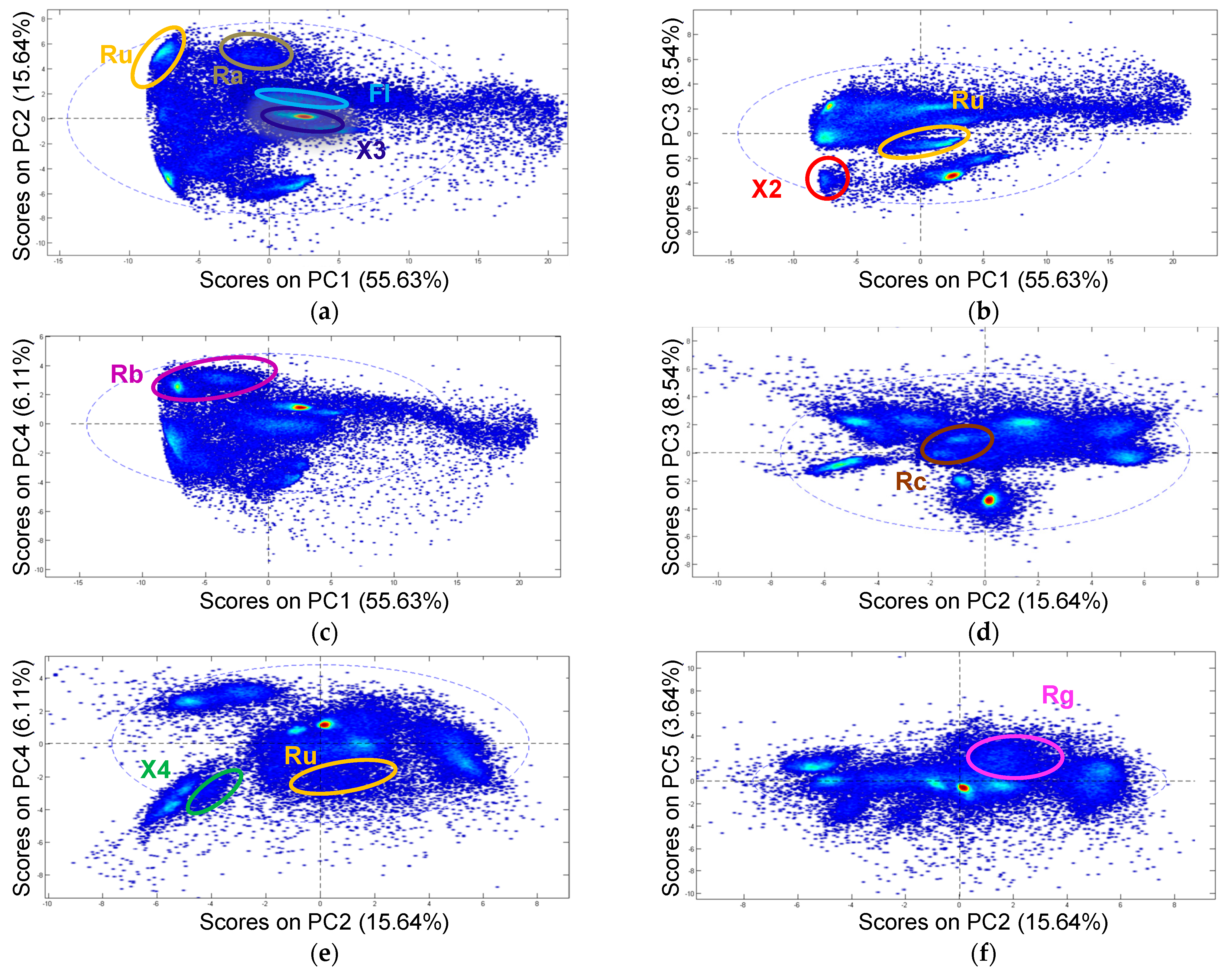
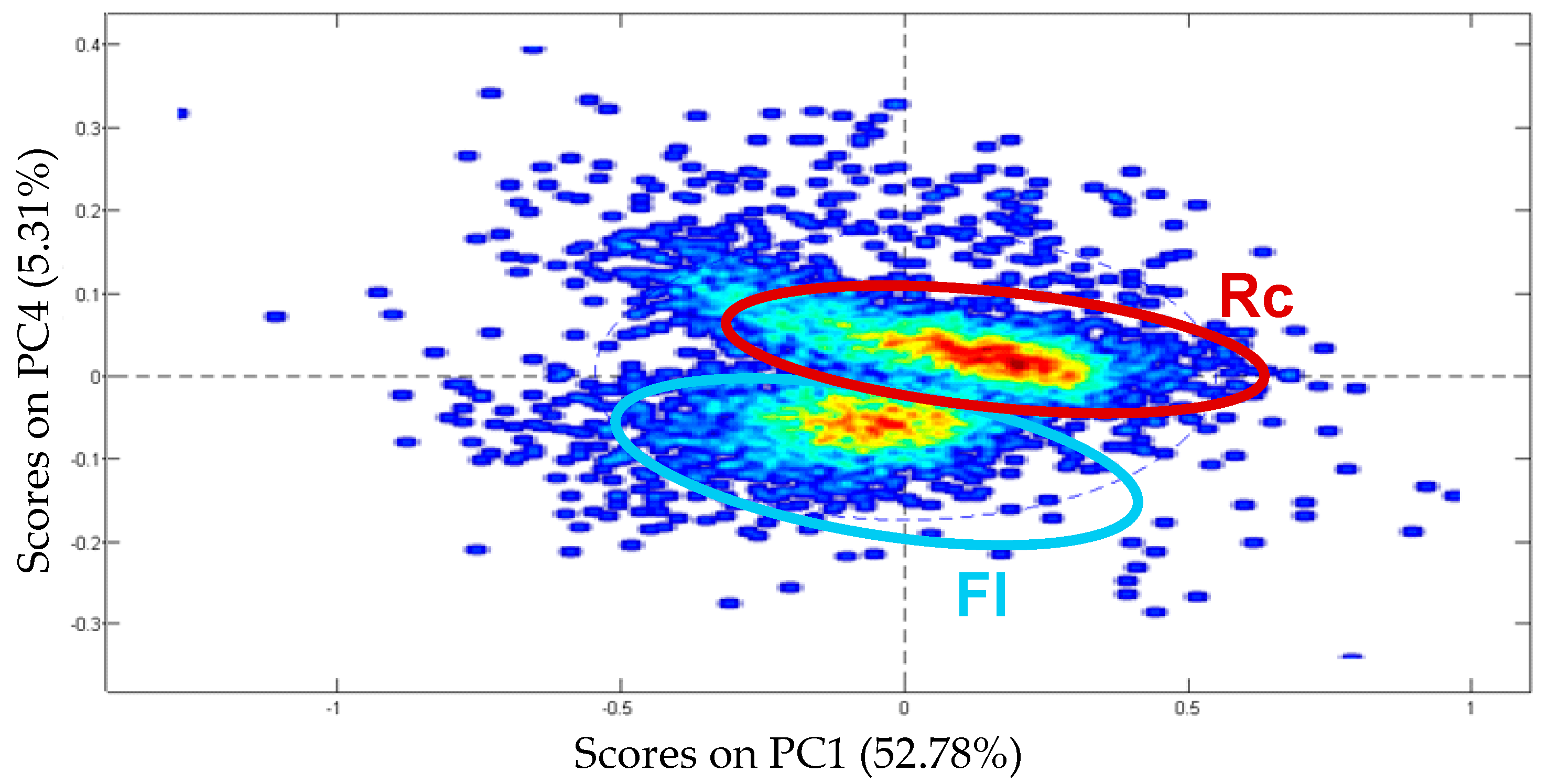
2.3.2. Principal Component Analysis (PCA)

PCA is an unsupervised method for reducing data dimensionality by projecting the samples into a low-dimensional subspace where the axes are called principal components (PCs) [33]. The PCs point in the direction of maximum variance.
Usually, the first principal component (PC1) accounts for the most variance in data, with significant variations indicated by the separation between points along PC1 and PC2.
The sample grouping into clusters in the PC space is an indicator of their similarity. The PCA scores plot can be used to visualize and understand existing relationships and/or patterns within the hyperspectral image or dataset. In the PCA scores plot, each data point (i.e., pixel or spectrum) from the original dataset is represented as a point.

2.3.3. Partial Least-Squares–Discriminant Analysis (PLS-DA)

Machine learning (ML) and deep learning (DL) algorithms are capable of analyzing hyperspectral data and autonomously label materials based on their different spectral patterns [34,35]. These algorithms allow us to precisely identify and classify materials after being trained with large databases of spectral fingerprints.
DL is a particular form of ML, which is inspired by the structure and function of the brain, attempting to replicate how the human brain learns. Artificial neural networks (ANNs)-based architectures are usually utilized to reach this goal. PLS-DA, ANN, convolutional neural network (CNN), naïve Bayes, decision trees (DT), k-nearest neighbor (k-NN), k-means clustering, classification and regression tree (CART), boosted regression tree (BRT), random forest (RF), and support vector machines (SVM) are among the most popular techniques used to manage multivariate datasets [34,35,36,37]. Image recognition and classification are the most common applications of ML and DL.
In this context, PLS-DA is considered one of the most suitable ML techniques for HSI analysis due to several key advantages. This multivariate approach is, in fact, a supervised classification method combining the properties of partial least-squares (PLS) regression analysis with the distinguishing ability of a classification technique [38]. This method is used to predict known classes in an unknown image, and it requires prior data knowledge (i.e., known samples are used to build the classification model). In more detail, PLS-DA aims to maximize the separation between different classes or groups in the data, providing interpretable results.
Classification models were trained by using preprocessed spectra extracted from ROIs or PCA score clusters. Venetian blinds (VBs) was chosen as cross-validation algorithm in order to assess the optimal complexity of the PLS-DA model [37]. PLS-DA classification performance is usually assessed using statistical parameters calculated from the confusion matrix of the classifier [39]. In this work, PLS-DA performance is reported in terms of Sensitivity and Specificity in calibration and cross-validation. The metric that evaluates a model’s ability to predict true positives in each available category is called Sensitivity, while Specificity measures a model’s ability to predict true negatives in each available category.

3. Experimental Results

3.1. Recyclable and Contaminant Materials Recognition (First Classification Strategy)

In order to set classes, ROIs were selected for the two-classes model (i.e., recyclable materials and contaminant materials) on the training image (Figure 3).
Preprocessing was applied to the ROIs’ collected spectra. The averaged raw and preprocessed spectra, obtained using the GLSW preprocessing algorithm, are reported in Figure 4. The selected preprocessing highlighted the spectral behavior of the two classes, allowing for an excellent PLS-DA classification in terms of prediction map, as shown in Figure 5.
The prediction results of the classification are very promising. It is easy to understand the correspondence existing between every object in the image and one of the two classes. Some pixel misclassifications are probably due to light scattering problems or the presence of fine particles (i.e., dust) on the particle surface. In Table 2, the Sensitivity and Specificity of the classification model are reported.
In order to perform the recognition of the four recyclable material classes and the identification of the five contaminant material classes individually, two different PLS-DA models were built.

3.1.1. Recyclable Materials Four-Classes Model

Starting from the training image, a subset of particles belonging to recyclable materials (i.e., Rc, Ru, Rb, and Ra) was selected. In order to correctly extract the significant spectral features, this new hyperspectral image was preprocessed, applying a sequential combination of three algorithms: derivative, SNV, and MC. The average raw and preprocessed spectra of concrete (Rc), aggregates (Ru), masonry (Rb), and hydrocarbon (Ra) are reported in Figure 6.
The absorption features, detectable around 1400 nm and 1900 nm in the spectra, are due to the O-H stretching and H-O-H bending vibrations in the water molecules [40]. Other absorption features in the Ru spectral signature around 2180–2220 nm can be related to Al-O-H, while 2250–2380 nm features in all the investigated spectra can be linked to Fe-O-H and/or Mg-O-H combination bands.
After preprocessing, an exploratory data analysis, based on PCA, was carried out. By analyzing the score plot of Figure 7, it is possible to distinguish, according to their grouping, different classes of products: PC2 and PC3 explaining 25.06% and 10.17% of the variance, respectively. Pixel grouping is an indicator of spectral similarity and can therefore reveal the variation in the chemical make-up of the samples even if they belong to the same set category. For instance, Ru (i.e., aggregate) shows more than one “pixel cloud” on the score plot, since particles belonging to Ru are probably not identical in terms of chemical composition.
The results achieved after the application of the PLS-DA model are shown in Figure 8. Satisfactory classification results were obtained, with excellent recognition of all four classes. Occurring pixel misclassifications are probably related to the particle edge effect and light scattering or due to the presence of extraneous inclusions in the particles. The Sensitivity and the Specificity parameters related to the developed model are reported in Table 3.

3.1.2. Contaminant Materials Five-Classes Model

Another subset of particles belonging to contaminant materials (i.e., Fl, Rg, X2, X3, and X4) was selected from the training image. The collected spectra were preprocessed using derivative and MC algorithms. In Figure 9, raw and preprocessed spectra are reported. Even in this case, preprocessing highlights spectral features. In addition to the spectra absorption related to the water presence (around 1400 nm and 1900 nm), other absorptions are related, in the cases of X2 and X3 samples, to the presence of lignin and cellulose [41].
Since not much information is available about the chemical composition of the other samples, it is not possible to associate all the spectra absorptions with a unique molecular bond. However, the SWIR range allows us to investigate material characteristics and status according to the presence of specific groups such as OH, NH, CH, SH, and CO.
PCA was applied, as explorative data analysis, after spectra preprocessing (Figure 10), and some pixels were selected onto the score plot in order to build the training dataset for the definition and the setup of the classification model. The best sample grouping was obtained by plotting PC1 and PC4 components: the first PC explains 67.29% of the data variance, while the fourth PC explains 3.37%.
The prediction image resulting from the application of the contaminant material model is reported in Figure 11. The classification results are satisfactory. Slight misclassifications occur along the particle boundaries, probably due to ragged particle edges. The Specificity and Sensitivity parameters of the PLS-DA model built to classify Fl, Rg, X2, X3 and X4 are reported in Table 4.

3.2. Single Material Classes Recognition (Second Classification Strategy)

After the removal of metal particles, the training image was used to define the nine-classes model able to identify Rc, Ru, Rb, Ra, Fl, Rg, X2, X3, and X4 at the same time. The original and the preprocessed average spectra obtained after the sequential application of the SNV, detrend, and MC algorithms are reported in Figure 12.
Even if it is quite difficult to perform a careful interpretation of acquired spectra behavior, the association of the main absorption bands to C-H, O-H, and N-H stretching vibrations is possible. In more detail, as mentioned before, the absorption features visible around 1400 nm and 1900 nm are due to the O-H stretching and H-O-H bending vibrations in the water molecules; meanwhile, the absorption around 2350 nm could be attributable to the calcite presence, which is one of the cement mortar constituents in the form of limestone and other forms of calcium carbonate [42]. Other absorption features in the spectral signatures around 2200–2400 nm can be related to the O-H combination bands. The preprocessing step can highlight the spectral behavior of the investigated samples.
PCA was applied after spectra preprocessing, and the different PC combinations obtained are reported in Figure 13. PC1 accounts for 55.63% of the variance, followed by PC2 (15.64%), PC3 (8.54%), PC4 (6.11%), and PC5 (3.54%). Starting from the analysis of the grouping of the different classes of materials on the score plots, the nine classes were set, and the training dataset for PLS-DA classification was built.
The results achieved after the nine-classes model application in terms of the prediction image are shown in Figure 14. The corresponding Specificity and Sensitivity parameters are reported in Table 5.
The classification produces good results with the exception of particles belonging to concrete (Rc class), which are confused with floating materials (Fl class), which are the autoclaved aerated concrete samples. Since Rc is a recyclable material, and Fl is a contaminant material, an adequate discrimination between these two classes is required; thus, a new PLS-DA model was built to achieve this goal.

Concrete and Floating Materials Model

Starting from the training image data set, particles belonging to Rc and Fl were cut, and a new training image was realized. Collected spectra were preliminarily preprocessed sequentially applying SNV, derivative and MC. In Figure 15, the raw and preprocessed spectra are reported.
PCA was applied after spectra preprocessing (Figure 16), and the two classes (i.e., Fl and Ru) are clustered in two groups on the PC1-PC4 score plot. The PC1 explains 52.78% of the data variance, while the PC4 explains the 5.31%.
After the application of the built PLS-DA onto the validation image constituted by Ru and Fl particles, a good classification was obtained (Figure 17). Statistical parameters relating to the efficiency of the built classification model (i.e., Sensitivity and Specificity) are reported in Table 6.

3.3. Results Comparison with Previous Benchmark Studies

The present findings obtained through two ad hoc classification strategies are in line with recent studies carried out by different authors, dealing with different C&DW materials. In a previous study [43], a PLS-DA classification strategy, adopting near-infrared (NIR)—HSI, was applied to C&DW materials. In more detail, a Sensitivity of 0.99, 1.00, 1.00, 1.00, 0.98, and 1.00 was reached for aggregates, brick, gypsum, plastic, wood, and foam classes, respectively.
Xiao et al. [26] designed an automatic sorting robot based on NIR hyperspectral images that was able to identify four different categories (i.e., wood, rubber, brick, concrete) adopting two different machine learning techniques. In more detail, they used extreme learning machine (ELM) and random forest (RF). Using ELM, a Sensitivity of 0.85, 0.96, 0.97, and 0.99 was obtained for wood, rubber, brick, and concrete, respectively, while using RF, a Sensitivity of 0.98, 0.94, 0.96, and 0.98 was obtained for wood, rubber, brick, and concrete, respectively.
Trotta et al. [28] obtained a PLS-DA Sensitivity ranging from 0.93 to 0.98 for the tile and cement mortar classes coming from post-earthquake building waste using SWIR-HSI.

4. Conclusions

A procedure based on HSI in the SWIR range (1000–2500 nm) was developed and different experimental set-ups were defined and implemented in order to recognize and classify different materials constituting DW.
Two different goals were achieved: (i) the recognition of contaminants in recyclable materials and (ii) the classification of each material category individually according to the technical specification EN 933-11:2009 [22]. In more detail, the goals were reached through two strategies:
  • Samples were first classified as recyclable (Class 1: Rc, Ru, Rb, and Ra) and contaminant (Class 2: Fl, Rg, X1, X2, X3, and X4) materials. Then, in a cascade detection perspective, the Rc, Ru, Rb, and Ra categories were correctly identified in the recyclable set and Fl, Rg, X1, X2, X3, and X4 were recognized in the contaminant material group.
  • All the samples (i.e., nine categories) were involved in the same classification model. Since some pixel misclassifications occur between concrete and floating materials, a two-classes model was built to recognize them.
Chemometric methods have been adopted to recognize the different classes of materials. PCA was applied to explore the data and set the classes, while PLS-DA was used to build classification models. The obtained results show that the applied techniques allow us to correctly identify the investigated categories in both the followed approaches, with Sensitivity and Specificity higher than 0.9 in all the built models.
As shown by the present findings, SWIR-HSI can be profitably utilized to discriminate different materials (i.e., recyclables and contaminants). Using this method, data may be acquired quickly, allowing for a significantly shorter analytical time and more effective and high-throughput analysis of samples. Moreover, such a non-destructive technique provides detailed spatial information, enabling the identification and recognition of the different materials in the C&DW stream. On the other hand, the limitations of SWIR-HSI for C&DW materials detection are mainly connected to sample conditions (i.e., sample overlapping can cause a blending of spectral fingerprints or the undetectability of the overlapped materials, making it difficult to identify separate components exactly) and instrumentation resolution (i.e., a limit on object size). Moreover, black or dark materials are difficult to identify via SWIR-his, since their spectral features may rely on subtle scattering effects.
Additionally, future studies should be conducted to attain a comprehensive characterization, encompassing both chemical and mechanical aspects, since it can be beneficial to ascertain the ultimate characteristics of the examined recyclable categories. In this context, efforts should be made to provide a thorough chemical characterization of the recycled materials by using X-ray fluorescence analysis.
The suggested strategy can be viewed as a methodological process to be applied consistently at the scale of recycling plants. In fact, the recycling process might be effectively automated by using these analytical techniques, supplementing or replacing human operations and sorting steps. This would result in a large cost decrease by improving and speeding up the recycling process.

Author Contributions

Conceptualization, G.B., S.S. and R.P.; methodology, R.P. and R.G.; software, R.P.; validation, R.P., G.B., G.H., H.B., R.G. and S.S.; formal analysis, R.P.; investigation, G.B., G.H., H.B., R.G., R.P. and S.S.; resources, G.H., H.B., G.B. and S.S.; data curation, R.G. and R.P.; writing—original draft preparation, R.P.; writing—review and editing, G.B., G.H., H.B., R.G., R.P. and S.S.; visualization, G.B. and S.S.; supervision, G.B. and S.S. All authors have read and agreed to the published version of the manuscript.

Funding

This research did not receive any specific grant from funding agencies in the public, commercial, or not-for-profit sectors.

Institutional Review Board Statement

Not applicable.

Informed Consent Statement

Not applicable.

Data Availability Statement

The data presented in this study are available on request from the corresponding authors.

Acknowledgments

The authors wish to thank Anna Angeluzzi for her support in HSI analyses.

Conflicts of Interest

The authors declare no conflict of interest.

References

  1. Eurostat. Waste Statistics in Europe. 2020. Available online: https://ec.europa.eu/eurostat/databrowser/view/cei_wm040/default/table?lang=en (accessed on 14 December 2022).
  2. Ossa, A.; García, J.; Botero, E. Use of recycled construction and demolition waste (CDW) aggregates: A sustainable alternative for the pavement construction industry. J. Clean. Prod. 2016, 135, 379–386. [Google Scholar] [CrossRef]
  3. Wang, T.; Wang, J.; Wu, P.; Wang, J.; He, Q.; Wang, X. Estimating the environmental costs and benefits of demolition waste using life cycle assessment and willingness-to-pay: A case study in Shenzhen. J. Clean. Prod. 2018, 172, 14–26. [Google Scholar] [CrossRef]
  4. Bonoli, A.; Zanni, S.; Serrano-Bernardo, F. Sustainability in Building and Construction within the Framework of Circular Cities and European New Green Deal. The Contribution of Concrete Recycling. Sustainability 2021, 13, 2139. [Google Scholar]
  5. European Commission. The European Green Deal; European Council: Brussels, Belgium, 2019.
  6. Ulsen, C.; Kahn, H.; Hawlitschek, G.; Masini, E.A.; Angulo, S.C. Separability studies of construction and demolition waste recycled sand. Waste Manag. 2013, 33, 656–662. [Google Scholar] [CrossRef]
  7. BRE. Recycled Aggregates. In BRE Digest 433, CI/SfB P(T6); Building Research Establishment: Watford, UK, 1998; p. 6. [Google Scholar]
  8. Silva, R.; De Brito, J.; Dhir, R. Properties and composition of recycled aggregates from construction and demolition waste suitable for concrete production. Constr. Build. Mater. 2014, 65, 201–217. [Google Scholar] [CrossRef]
  9. Silva, R. Use of Recycled Aggregates from Construction and Demolition Waste in the Production of Structural Concrete. Ph.D. Thesis, Instituto Superior Tecnico, Lisboa, Portugal, 2015. [Google Scholar]
  10. Martín-Morales, M.; Zamorano, M.; Ruiz-Moyano, A.; Valverde-Espinosa, I. Characterization of recycled aggregates construction and demolition waste for concrete production following the Spanish Structural Concrete Code EHE-08. Constr. Build. Mater. 2011, 25, 742–748. [Google Scholar] [CrossRef]
  11. Zhang, C.; Hu, M.; Di Maio, F.; Sprecher, B.; Yang, X.; Tukker, A. An overview of the waste hierarchy framework for analyzing the circularity in construction and demolition waste management in Europe. Sci. Total Environ. 2022, 803, 149892. [Google Scholar] [CrossRef]
  12. Mrad, C.; Frölén Ribeiro, L. A Review of Europe’s Circular Economy in the Building Sector. Sustainability 2022, 14, 14211. [Google Scholar] [CrossRef]
  13. Joseph, H.S.; Pachiappan, T.; Avudaiappan, S.; Maureira-Carsalade, N.; Roco-Videla, Á.; Guindos, P.; Parra, P.F. A Comprehensive Review on Recycling of Construction Demolition Waste in Concrete. Sustainability 2023, 15, 4932. [Google Scholar] [CrossRef]
  14. Angulo, S.C.; Carrijo, P.M.; Figueiredo, A.D.; Chaves, A.P.; John, V.M. On the classification of mixed construction and demolition waste aggregate by porosity and its impact on the mechanical performance of concrete. Mater. Struct. 2010, 43, 519–528. [Google Scholar] [CrossRef]
  15. Pereira, P.M.; Vieira, C.S. A Literature Review on the Use of Recycled Construction and Demolition Materials in Unbound Pavement Applications. Sustainability 2022, 14, 13918. [Google Scholar] [CrossRef]
  16. Dosho, Y. Development of a sustainable concrete waste recycling system-Application of recycled aggregate concrete produced by aggregate replacing method. J. Adv. Concr. Technol. 2007, 5, 27–42. [Google Scholar] [CrossRef]
  17. Eguchi, K.; Teranishi, K.; Nakagome, A.; Kishimoto, H.; Shinozaki, K.; Narikawa, M. Application of recycled coarse aggregate by mixture to concrete construction. Constr. Build. Mater. 2007, 21, 1542–1551. [Google Scholar] [CrossRef]
  18. Lotfi, S.; Deja, J.; Rem, P.; Mróz, R.; van Roekel, E.; van der Stelt, H. Mechanical recycling of EOL concrete into high-grade aggregates. Resour. Conserv. Recycl. 2014, 87, 117–125. [Google Scholar] [CrossRef]
  19. Chini, A.R.; Bruening, S. Deconstruction and materials reuse in the United States. Future Sustain. Constr. 2003, 14, 1–22. [Google Scholar]
  20. Gebremariam, A.T.; Di Maio, F.; Vahidi, A.; Rem, P. Innovative technologies for recycling End-of-Life concrete waste in the built environment. Resour. Conserv. Recycl. 2020, 163, 104911. [Google Scholar] [CrossRef]
  21. Ferrández, D.; Saiz, P.; Zaragoza-Benzal, A.; Zúñiga-Vicente, J.A. Towards a more sustainable environmentally production system for the treatment of recycled aggregates in the construction industry: An experimental study. Heliyon 2023, 9, e16641. [Google Scholar] [CrossRef]
  22. NBN EN 933-11:2009; Tests for Geometrical Properties of Aggregates—Part 11: Classification Test for the Constituents of Coarse Recycled Aggregate. Comité Européen de Normalisation: Brussels, Belgium, 2009.
  23. Hyvarinen, T.S.; Herrala, E.; Dall’Ava, A. Direct sight imaging spectrograph: A unique add-in component brings spectral imaging to industrial applications. In Digital Solid State Cameras: Designs and Applications; International Society for Optics and Photonics: Bellingham, WA, USA, 1998. [Google Scholar]
  24. Geladi, P.; Grahn, H.; Burger, J. Multivariate images, hyperspectral imaging: Background and equipment. In Techniques and Applications of Hyperspectral Image Analysis; Wiley: Hoboken, NJ, USA, 2007; pp. 1–15. [Google Scholar]
  25. Bonifazi, G.; Palmieri, R.; Serranti, S. Hyperspectral imaging applied to end-of-life (EOL) concrete recycling. Tm-Tech. Mess. 2015, 82, 616–624. [Google Scholar] [CrossRef]
  26. Xiao, W.; Yang, J.; Fang, H.; Zhuang, J.; Ku, Y.; Zhang, X. Development of an automatic sorting robot for construction and demolition waste. Clean Technol. Environ. Policy 2020, 22, 1829–1841. [Google Scholar] [CrossRef]
  27. Hollstein, F.; Cacho, Í.; Arnaiz, S.; Wohllebe, M. Challenges in automatic sorting of construction and demolition waste by hyperspectral imaging. In Advanced Environmental, Chemical, and Biological Sensing Technologies; SPIE: Baltimore, MD, USA, 2016; Volume 9862, pp. 73–82. [Google Scholar]
  28. Trotta, O.; Bonifazi, G.; Capobianco, G.; Serranti, S. Recycling-Oriented Characterization of Post-Earthquake Building Waste by Different Sensing Techniques. J. Imaging 2021, 7, 182. [Google Scholar] [CrossRef]
  29. Rinnan, Å.; Van Den Berg, F.; Engelsen, S.B. Review of the most common pre-processing techniques for near-infrared spectra. TrAC Trends Anal. Chem. 2009, 28, 1201–1222. [Google Scholar] [CrossRef]
  30. Tauler, R.; Peré-Trepat, E.; Lacorte, S.; Barceló, D. Chemometrics modelling of environmental data. In Proceedings of the 2nd International Congress on Environmental Modelling and Software, Osnabrück, Germany, 14–17 June 2004. [Google Scholar]
  31. Wise, B.M.; Gallagher, N.B.; Bro, R.; Shaver, J.M.; Windig, W.; Koch, R.S. Chemometrics Tutorial for PLS_Toolbox and Solo; Eigenvector Research, Inc.: Wenatchee, WA, USA, 2006; Volume 3905, pp. 102–159. [Google Scholar]
  32. Martens, H.; Høy, M.; Wise, B.M.; Bro, R.; Brockhoff, P.B. Pre-whitening of data by covariance-weighted pre-processing. J. Chemom. J. Chemom. Soc. 2003, 17, 153–165. [Google Scholar] [CrossRef]
  33. Wold, S.; Esbensen, K.; Geladi, P. Principal component analysis. Chemom. Intell. Lab. Syst. 1987, 2, 37–52. [Google Scholar] [CrossRef]
  34. Gewali, U.B.; Monteiro, S.T.; Saber, E. Machine learning based hyperspectral image analysis: A survey. arXiv 2018, arXiv:1802.08701. [Google Scholar]
  35. Paoletti, M.E.; Haut, J.M.; Plaza, J.; Plaza, A. Deep learning classifiers for hyperspectral imaging: A review. ISPRS J. Photogramm. Remote Sens. 2019, 158, 279–317. [Google Scholar] [CrossRef]
  36. Manna, T.; Anitha, A. Deep Ensemble-Based Approach Using Randomized Low-Rank Approximation for Sustainable Groundwater Level Prediction. Appl. Sci. 2023, 13, 3210. [Google Scholar] [CrossRef]
  37. Anitha, A.; Shivakumara, P.; Jain, S.; Agarwal, V. Convolution Neural Network and Auto-encoder Hybrid Scheme for Automatic Colorization of Grayscale Images. In Smart Computer Vision; Springer: Berlin/Heidelberg, Germany, 2023; pp. 253–271. [Google Scholar]
  38. Barker, M.; Rayens, W. Partial least squares for discrimination. J. Chemom. J. Chemom. Soc. 2003, 17, 166–173. [Google Scholar] [CrossRef]
  39. Fawcett, T. An introduction to ROC analysis. Pattern Recognit. Lett. 2006, 27, 861–874. [Google Scholar] [CrossRef]
  40. Crowley, J.; Williams, D.; Hammarstrom, J.; Piatak, N.; Chou, I.-M.; Mars, J. Spectral reflectance properties (0.4–2.5 μm) of secondary Fe-oxide, Fe-hydroxide, and Fe-sulphate-hydrate minerals associated with sulphide-bearing mine wastes. Geochem. Explor. Environ. Anal. 2003, 3, 219–228. [Google Scholar] [CrossRef]
  41. Schwanninger, M.; Rodrigues, J.C.; Fackler, K. A review of band assignments in near infrared spectra of wood and wood components. J. Near Infrared Spectrosc. 2011, 19, 287–308. [Google Scholar] [CrossRef]
  42. Bonifazi, G.; Palmieri, R.; Serranti, S. Evaluation of attached mortar on recycled concrete aggregates by hyperspectral imaging. Constr. Build. Mater. 2018, 169, 835–842. [Google Scholar] [CrossRef]
  43. Bonifazi, G.; Capobianco, G.; Palmieri, R.; Serranti, S.S. Hyperspectral imaging applied to the waste recycling sector. Spectrosc. Eur. 2019, 31, 8–11. [Google Scholar] [CrossRef]
Figure 1. Digital images of the training (a) and validation set (b). The analyzed categories are concrete (Rc), aggregates (Ru), masonry (Rb), hydrocarbons (Ra), floating materials (autoclaved aerated concrete) (Fl), glass (Rg), metals (X1), wood (X2), cardboard (X3), and parget (X4).
Sustainability 15 15009 g001
Figure 2. Block diagram showing the strategies followed to define the different classification models. For the “model a”, regions of interest (ROIs) were selected to set the classes from the training image, while for the “model b”, training dataset was obtained by selecting pixels belonging to each different investigated category on PCA score plot.
Sustainability 15 15009 g002
Figure 3. Example of different regions of interest (ROIs) selection for class for the two-classes model (i.e., recyclable and contaminants recognition).
Sustainability 15 15009 g003
Figure 4. Raw (a) and preprocessed (b) spectra of recyclable and contaminant materials contained in the analyzed C&DW samples.
Sustainability 15 15009 g004
Figure 5. Prediction map resulting from the application of the 2-classes PLS-DA model to the validation image shown in Figure 1b. The two classes are “recyclable materials” (dark red) and “contaminant materials” (dark blue).
Sustainability 15 15009 g005
Figure 6. Raw (a) and preprocessed (b) spectra of Rc (i.e., concrete, mortar), Ru (i.e., natural stones, aggregates), Rb (i.e., masonry, mainly bricks, tiles, and ceramics), and Ra (i.e., hydrocarbons).
Sustainability 15 15009 g006
Figure 7. PC2-PC3 score plot showing the data point clustering of 4 classes of materials (i.e., Rc, Ru, Rb, and Ra).
Sustainability 15 15009 g007
Figure 8. Digital image (a) and corresponding prediction map (b) resulting from the application of the 4-classes PLS-DA model for recyclable materials. The 4 classes are “Rc” (dark red), “Ra” (yellow), “Ru” (cyan), and “Rb” (dark blue).
Sustainability 15 15009 g008
Figure 9. Raw (a) and preprocessed (b) spectra of Fl (i.e., floating materials), Rg (i.e., glass), X2 (i.e., wood), X3 (i.e., cardboard), and X4 (i.e., parget).
Sustainability 15 15009 g009
Figure 10. PC1-PC4 score plot showing the data point clustering of 5 classes of materials (i.e., Fl, Rg, X2, X3, and X4).
Sustainability 15 15009 g010
Figure 11. Source digital image set (a) and corresponding prediction map (b) resulting from the application of the 5-classes PLS-DA model for contaminant materials. The 5 classes are “Fl” (green), “Rg” (dark red), “X2” (dark cyan), “X3” (dark blue), and “X4” (orange).
Sustainability 15 15009 g011aSustainability 15 15009 g011b
Figure 12. Raw (a) and preprocessed (b) spectra of Rc, Ru, Rb, Ra, Fl, Rg, X2, X3, and X4 samples.
Sustainability 15 15009 g012
Figure 13. Different combinations of PC score plots showing the spatial position of the different classes of materials after the application of preprocessing algorithms and the identification of pixels belonging to each class: PC1-PC2 (a), PC1-PC3 (b), PC1-PC4 (c), PC2-PC3 (d), PC2-PC4 (e), and PC2-PC5 (f).
Sustainability 15 15009 g013
Figure 14. Source digital image set (a) and corresponding prediction map (b) resulting from the application of the 9-classes PLS-DA model for contaminant materials. The 9 classes are “Rc” (orange), “Ru” (blue), “Rb” (yellow), “Ra” (dark blue), “Fl” (dark cyan), “Rg” (dark red), “X2” (green), “X3” (cyan), and “X4” (red).
Sustainability 15 15009 g014
Figure 15. Raw (a) and preprocessed (b) spectra of Rc and Fl samples.
Sustainability 15 15009 g015
Figure 16. PC1-PC4 score plot showing the clustering of the 2 classes of materials (i.e., Fl and Ru).
Sustainability 15 15009 g016
Figure 17. Source digital image set (a) and corresponding prediction map (b) resulting from the application of the 2-classes PLS-DA model for concrete and floating materials. The 2 classes are “Rc” (blue) and “Fl” (red).
Sustainability 15 15009 g017
Table 1. Adopted identification and description of the sinking and floating materials as resulting from hydraulic separation.
Identification CodeConditionDescription
RecyclablesRcNon-floatingConcrete and mortar
RuNon-floatingNatural stones and aggregates
RbNon-floatingMasonry (i.e., bricks, tiles, ceramics, etc.)
RaNon-floatingHydrocarbons
ContaminantsRgNon-floatingGlass
X1Non-floatingMetals (ferrous and non-ferrous)
X2Non-floatingNon-floating wood
X3Non-floatingCardboard
X4Non-floatingParget, gypsum plaster
FlFloatingAutoclaved aerated concrete
Table 2. Sensitivity and Specificity values of PLS-DA model built to recognize recyclable and contaminant materials.
Contaminant
Materials
Recyclable
Materials
SensitivityCalibration0.9640.974
Cross-validation0.9420.962
SpecificityCalibration0.9740.964
Cross-validation0.9620.942
Table 3. Sensitivity and Specificity values of PLS-DA model built to recognize Rc, Ru, Rb, and Ra classes of materials.
RcRuRbRa
SensitivityCalibration0.9740.9821.0001.000
Cross-validation0.9730.9811.0001.000
SpecificityCalibration0.9860.9941.0000.981
Cross-validation0.9850.9951.0000.981
Table 4. Sensitivity and Specificity values of PLS-DA model built to recognize Fl, Rg, X2, X3, and X4 sample.
FlRgX2X3X4
SensitivityCalibration1.0001.0000.9991.0001.000
Cross-validation1.0001.0000.9991.0001.000
SpecificityCalibration1.0001.0000.9931.0000.997
Cross-validation1.0001.0000.9921.0000.997
Table 5. Sensitivity and Specificity values of PLS-DA model built to recognize Rc, Ru, Rb, Ra, Fl, Rg, X2, X3, and X4 samples.
RcRuRbRaFlRgX2X3X4
SensitivityCalibration0.9830.9970.9941.0000.9860.9980.9990.9750.995
Cross-validation0.9830.9970.9921.0000.9860.9980.9990.9750.995
SpecificityCalibration0.9970.9880.9961.0000.9950.9990.9890.9750.994
Cross-validation0.9970.9880.9961.0000.9950.9990.9890.9750.994
Table 6. Sensitivity and Specificity values of PLS-DA model built to recognize Rc and Fl.
RcFl
SensitivityCalibration0.9990.997
Cross-validation0.9990.997
SpecificityCalibration0.9970.999
Cross-validation0.9970.999
Disclaimer/Publisher’s Note: The statements, opinions and data contained in all publications are solely those of the individual author(s) and contributor(s) and not of MDPI and/or the editor(s). MDPI and/or the editor(s) disclaim responsibility for any injury to people or property resulting from any ideas, methods, instructions or products referred to in the content.

