Article

Hyperspectral Imaging Applied to WEEE Plastic Recycling: A Methodological Approach

by
Giuseppe Bonifazi
1,2,
Ludovica Fiore
1,
Riccardo Gasbarrone
3,
Roberta Palmieri
1,* and
Silvia Serranti
1,2
1
Department of Chemical Engineering, Materials and Environment, Sapienza University of Rome, 00184 Rome, Italy
2
Research Center for Biophotonics, Sapienza University of Rome, 04100 Latina, Italy
3
Research and Service Center for Sustainable Technological Innovation, Sapienza University of Rome, 04100 Latina, Italy
*
Author to whom correspondence should be addressed.
Sustainability 2023, 15(14), 11345; https://doi.org/10.3390/su151411345
Submission received: 5 June 2023 / Revised: 18 July 2023 / Accepted: 19 July 2023 / Published: 21 July 2023
(This article belongs to the Special Issue Hyperspectral Imaging for Sustainable Waste Recycling)

Abstract

:
In this study, the possibility of applying the hyperspectral imaging (HSI) technique in the Short-Wave InfraRed (SWIR) spectral range to characterize polymeric parts coming from Waste from Electric and Electronic Equipment (WEEE) is explored. Different case studies are presented referring to the identification of (i) plastic flakes inside a mixed waste stream coming from a recycling plant of monitors and flat screens, (ii) different polymers inside a mixed plastic waste stream coming from End-Of-Life (EOL) electronic device housings and trims, (iii) contaminants (i.e., metals) in a mix of shredded plastic particles coming from a recycling line of electrical cables, and (iv) brominated plastics in mixed streams constituted by small appliances (i.e., cathode-ray tube televisions and monitors). The application of chemometric techniques to hyperspectral data demonstrated the potentiality of this approach for systematic utilization for material characterization, quality control and sorting purposes. The experimental findings highlight the feasibility of employing this method due to its user-friendly nature and quick detection response. To increase and optimize WEEE valorization avoiding disposal in landfills or incineration, recycling-oriented characterization and/or quality control of the processed products are fundamental to identify and quantify substances to be recovered.

1. Introduction

The widespread presence and use of Electrical and Electronic Equipment (EEE) has become an integral part of modern life. This accessibility and widespread adoption have considerably improved the quality of life for a sizable segment of the worldwide population [1]. However, the way we generate, use and dispose of e-waste is often not sustainable. In the last few decades, the manufacture of EEE has become one of the fastest-expanding industrial sectors due to the rapid advancement of technology. One consequence of the progress in the technology sector is the increased production of Waste from Electrical and Electronic Equipment (WEEE) [2], also due to the fact that most consumers tend to discard their devices very often because they are perceived as obsolete. Moreover, considering that WEEE has intrinsic potential toxicity for environment and human/animal health, special treatments are needed in order to manage these materials, mostly from recycling and recovery perspectives [3]. Consequently, many countries have to face the significant environmental and human health risks posed by improperly managed WEEE [1]. Unsafe treatment and improper disposal of WEEE pose substantial problems for the accomplishment of the Sustainable Development Goals (SDGs) identified in the 2030 Agenda for Sustainable Development adopted by the United Nations and all European member states [1].
On the other hand, WEEE contains precious and critical elements (i.e., gold, silver, copper, rare earths, etc.) as well as other important materials such as plastic, glass and wood that, if correctly managed, can become secondary raw materials to be placed on the market again [4].
Plastic, which is becoming more and more relevant for recovery or material recycling systems, is one of the most common materials found in WEEE, being on average 10–30% [5]. Polymers are usually used for electronic equipment housings because they exhibit excellent properties and are relatively inexpensive. Typically, polymers have such meritorious features such as lightness, high flexibility, workability at low temperatures, and low electrical and thermal conductivity. The use of additives can further enhance these characteristics (i.e., fillers, fibers, carbon black and plasticizers).
Acrylonitrile/butadiene/styrene (ABS), polypropylene (PP), high-impact polystyrene (HIPS) and polyphenylene oxide/high-impact polystyrene (PPO/HIPS) are the most common polymers used in EEE [6]. Polycarbonate (PC) and PC/ABS mixtures are increasingly being used today. Table 1 lists several polymer types employed in electrical and electronic equipment, along with their applications [7].
In 2020, 29.5 million tons of post-consumer plastic waste were collected in the European Union, including Norway, Switzerland and the United Kingdom (EU27 + 3) [8]. This volume is approximately 1% of the entire amount of post-consumer waste generated in the EU27 + 3 in the same year (e.g., organic waste, glass, paper, metals, wood, cardboard, concrete, etc.). The majority of post-consumer plastic waste collected in 2020 came from packaging, accounting for 61% of the total. This was followed by waste from construction and building-related applications at 6% and waste from electrical and electronic applications, which accounted for 6%.
Over 10 million tons of post-consumer plastic were recycled in 2020. But in the same year, 65% of the collected plastic waste was not valorized in a circular economy approach [4]. The employment of expensive and/or complex machinery in the recycling industry is problematic mainly due to a wide range of technical (such as particles of various sizes, shapes, compositions and physical conditions of the waste to be processed), environmental (such as harsh operational environments) and financial (e.g., low values of recovered materials or products) factors.
As a consequence, efficient and cost-effective solutions are necessary for material characterization, quality control of recycled products and sorting applications. The use of Hyperspectral Imaging (HSI)-based sensors working in the Short-Wave InfraRed (SWIR) spectral range can be a viable solution to this challenge. HSI is a cutting-edge approach to waste management that is rapidly gaining popularity as a quality control tool and as a core for sorting engines in several recycling processes [9]. Different HSI-based approaches have been proposed for plastic recycling [10,11,12], Construction and Demolition Waste (C&DW) recycling [13,14] and WEEE recycling [15,16].
In this work, a methodological approach based on the utilization of SWIR-HSI techniques for both sorting and/or quality control applications of different plastic streams from WEEE is presented.

2. Hyperspectral Imaging

Hyperspectral imaging (HSI) is a method combining digital imaging with conventional spectroscopy to simultaneously acquire spatial and spectral data of the materials being analyzed [17,18]. This information is stored in a three-dimensional dataset known as a “hypercube,” where two dimensions (x, y) represent spatial information and the third provides spectral data. In addition to the morphological properties of the investigated sample as a conventional image, a hypercube also contains its physical and chemical characteristics, which can be examined based on the specific wavelengths under investigation. Thus, a complete spectrum is obtained for each pixel, and depending on the various wavelengths under investigation, each pixel provides information about different sample physico-chemical properties.
In terms of material characterization and product quality control, HSI enables, inside a WEEE stream, the identification of plastic, the recognition of polymers and contaminant detection [12,19,20].

2.1. Hyperspectral Imaging System and Data Handling

The HSI analyses were carried out at the Raw Materials Laboratory (RawMaLab) of the Department of Chemical Engineering, Materials & Environment located at Sapienza University of Rome (Rome, Italy). The adopted equipment was the SisuCHEMA XL™ Chemical Imaging workstation (Specim Spectral Imaging Oy Ltd., Oulu, Finland). This system consists of a CCD camera and a Specim ImSpector N25E spectrograph, operating in the SWIR region of the electromagnetic spectrum (1000–2500 nm), with a spectral resolution of 10 nm and spectral/pixel sampling of 6.3 nm, a mobile platform on which the samples can be positioned, a halogen source lighting system and an integrated white calibration system that allows optimization of the focus lens. The entire system is controlled by a personal computer with the Specim ChemaDAQ™ software for spectra acquisition and collection. The HSI-employed platform operates as a line scan camera of the push-broom type, enabling the capture of spectral data for every pixel along the scanning line.
Calibration is performed automatically by the ChemaDAQ™ software. The calibration procedure involves capturing a dark image ( D ), recording an image obtained by closing the camera shutter and measuring a white spectral reflectance standard by collecting the white reference image ( W ). After this calibration phase, the raw hyperspectral image ( R 0 ) is acquired, and the reflectance image ( R ) of the acquired image is then calculated, thanks to the equation:
R = R 0 D W D
PLS_Toolbox (Ver 9.0; Eigenvector Research, Inc., Wenatchee, WA, USA) and MIA_toolbox (Ver 3.1; Eigenvector Research, Inc., Wenatchee, WA, USA) running in the MATLAB® (R2021b Ver. 9.11; The Mathworks, Inc., Natick, MA, USA) environment were adopted to handle and analyze hypercubes.

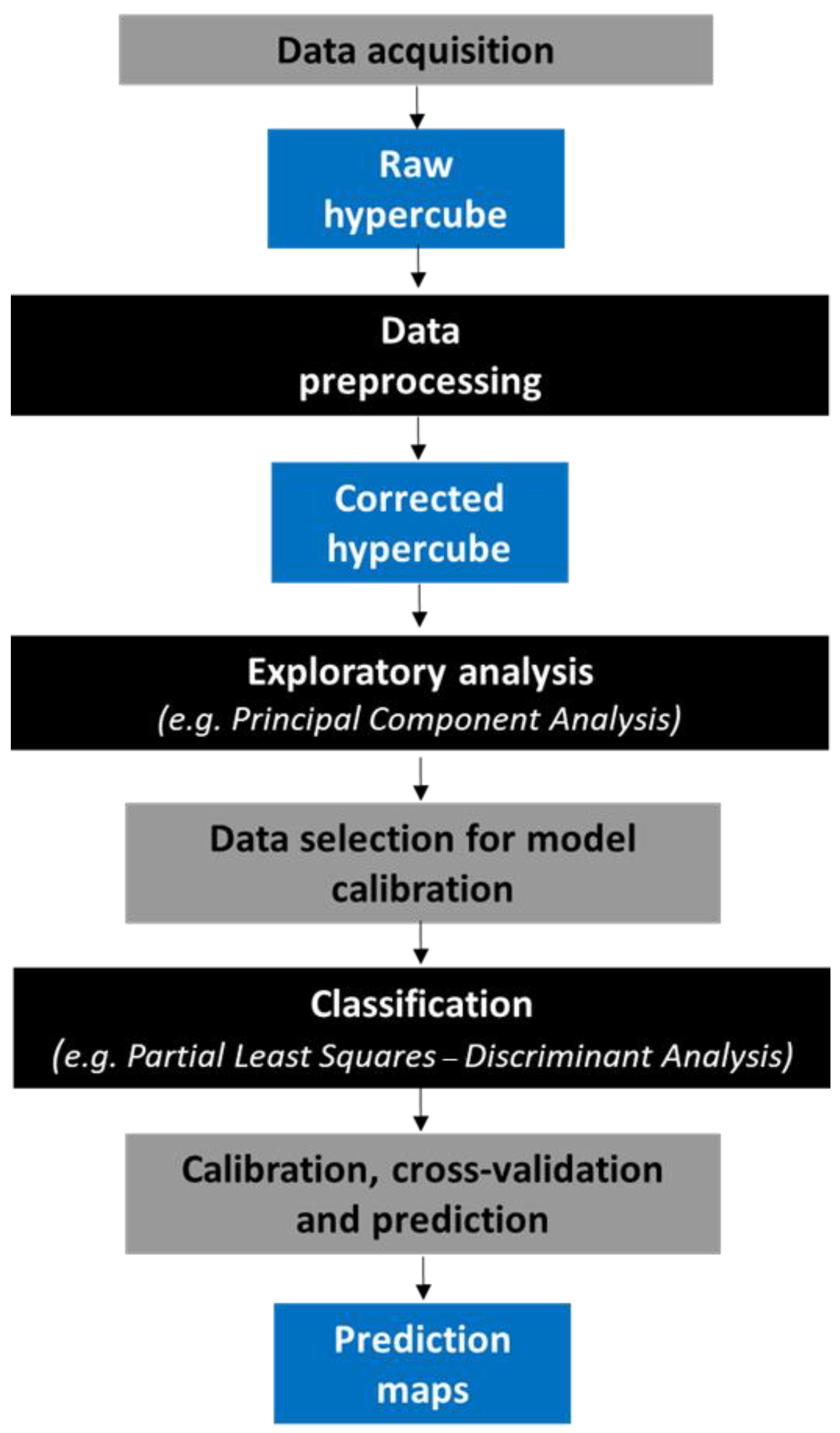
2.2. Hyperspectral Images Analysis Procedure

Hyperspectral images typically contain many spectra and are very informative. The main purpose of hyperspectral image analysis is usually to reduce its size while maintaining sufficient information to identify, classify and/or quantify the areas of a sample from a physico-chemical point of view [21,22]. The analysis of hyperspectral data is based on techniques that combine signal processing, image processing and spectroscopy.
Starting from the raw data of the hypercube, a data preprocessing phase is necessary to remove unwanted variations from the spectral information and to prepare the data for further processing. These artifacts (i.e., dead pixels and spikes) must be identified and excluded from subsequent analyses [21]. Following the identification and correction of these causes of variation in the data, or alternatively, downstream of this approach, it may be essential to remove the image’s background (i.e., the portion of the image that does not contain the sample).
Once the hypercube data has been preprocessed, the next stage of investigation commonly followed is exploratory analysis [22]. Exploratory analysis is a qualitative tool. Principal Component Analysis (PCA) is a basic chemometric approach useful to perform an exploratory analysis of HSI data, allowing to investigate all possible sources of variability within a hypercube. The purpose of this multivariate analysis technique is to reduce the number of variables describing a data matrix to a smaller number of Principal Components (PCs), which are a linear combination of the original descriptors (experimental variables), limiting the loss of information as much as possible [23].
To classify the data of a hypercube, it is necessary to develop a robust and reliable model. Certain regions of the image, or Regions of Interest (ROIs), which are subsets of spectra, can be utilized to calibrate a classification model. There are many pixel-based or object-based classification techniques, including unsupervised methods (such as K-Nearest Neighbors (k-NN)) and supervised methods (i.e., Partial Least Squares–Discriminant Analysis (PLS-DA)).
A prediction map can be obtained from any model developed from spectral data by applying it to each pixel in a hypercube.
The HSI methodology presented in this work follows the steps shown in the diagram presented in Figure 1. ROIs were selected on each acquired particle in the hyperspectral images. Spectra obtained from ROIs were then compared with reference spectra in order to perform a preliminary sample identification.
PCA was adopted as an exploratory analysis of reference plastic spectra. The classes required for the following classification tasks were defined as a result of this investigation.
A classification procedure based on Partial Least Squares–Discriminant Analysis (PLS-DA) was then adopted, depending on the goal of the study. The PLS-DA, which is related to another classification technique called Linear Discriminant Analysis (LDA), is essentially an extension of Partial Least Squares (PLS) regression for classification purposes [24]. The model was validated by applying it to the hyperspectral images.
The confusion matrix is assessed to determine how well a supervised classifier performs [25]. Among the most important parameters that can be calculated starting from the confusion matrix are Sensitivity, defined by Equation (2), which measures the ability of the system to identify instances of the positive class (i.e., the percentage of instances classified as positive among all the instances that are actually positive), and Specificity, calculated on the basis of the negative class with Equation (3). The PLS-DA classifications were evaluated in terms of Sensitivity and Specificity.
Both Sensitivity and Specificity have values ranging from 0 to 1. A Sensitivity of 1 means the model properly recognized all positive instances, while a Specificity of 1 means the model correctly identified all negative instances. A Sensitivity or Specificity of 0, on the other hand, indicates that the model failed to identify any positive or negative instances.
The PLS-DA classifications were evaluated in terms of Sensitivity and Specificity.
S e n s i t i v i t y = T r u e   P o s i t i v e ( T r u e   P o s i t i v e + F a l s e   N e g a t i v e )
S p e c i f i c i t y = T r u e   N e g a t i v e ( T r u e   P o s i t i v e + F a l s e   N e g a t i v e )

3. Case Studies

Four different case studies were investigated, related to different WEEE waste streams containing plastics and their potential recycling. In all cases, samples have been collected from different recycling plants and represent real current critical issues for the recycling of plastic fractions from other materials (i.e., identification for sorting and/or quality control purposes).

3.1. Plastic Flake Identification in Mixed Waste from EOL Monitors and Flat Screens

3.1.1. Analyzed Samples and Procedure Set-Up

In this case study, the analyzed sample comes from a milling process of mixed waste from EOL monitors and flat screens. A procedure was developed in order to recognize plastic flakes from other materials (mainly constituted by fragments of Printed Circuit Boards (PCBs) and various metal particles).
The process of sample selection involved the utilization of coning and quartering procedure, followed by a subsequent manual sorting stage.
Particles were categorized into two classes: (1) Plastic class, 68% in weight of the sample (wt%), and (2) Other class (i.e., fragments of PCBs and mixed metal particles; 32 wt%). ROIs of Plastic and Other particles were selected in order to calibrate a PLS-DA classifier. Reflectance spectra extracted from ROIs were preprocessed with Standard Normal Variate (SNV) and Mean Center (MC). The SNV algorithm is a weighted normalization approach [26], whereas MC, one of the most often used preprocessing techniques, computes the column mean and subtracts it from the column value. PCA was adopted in order to explore the calibration data and identify and exclude outliers. Finally, PLS-DA was applied to recognize the two classes.

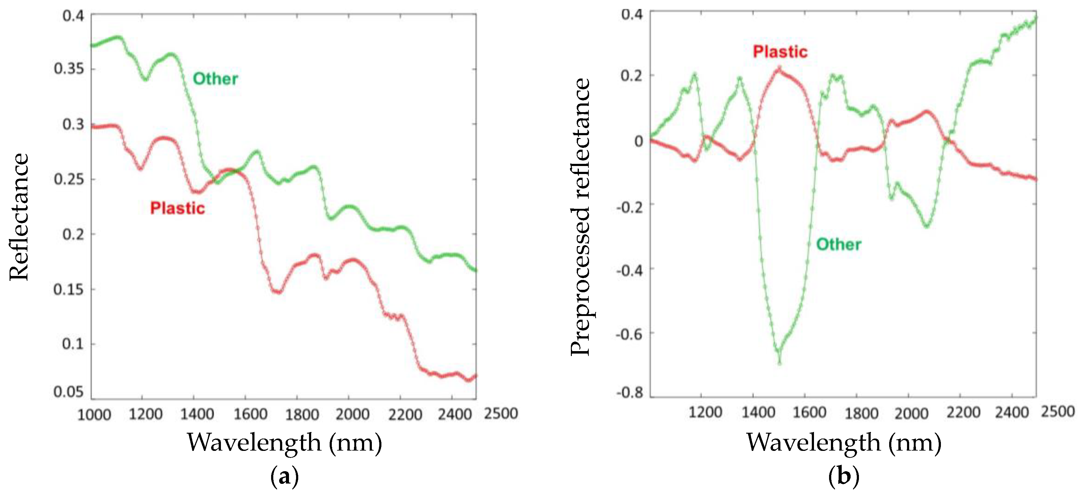
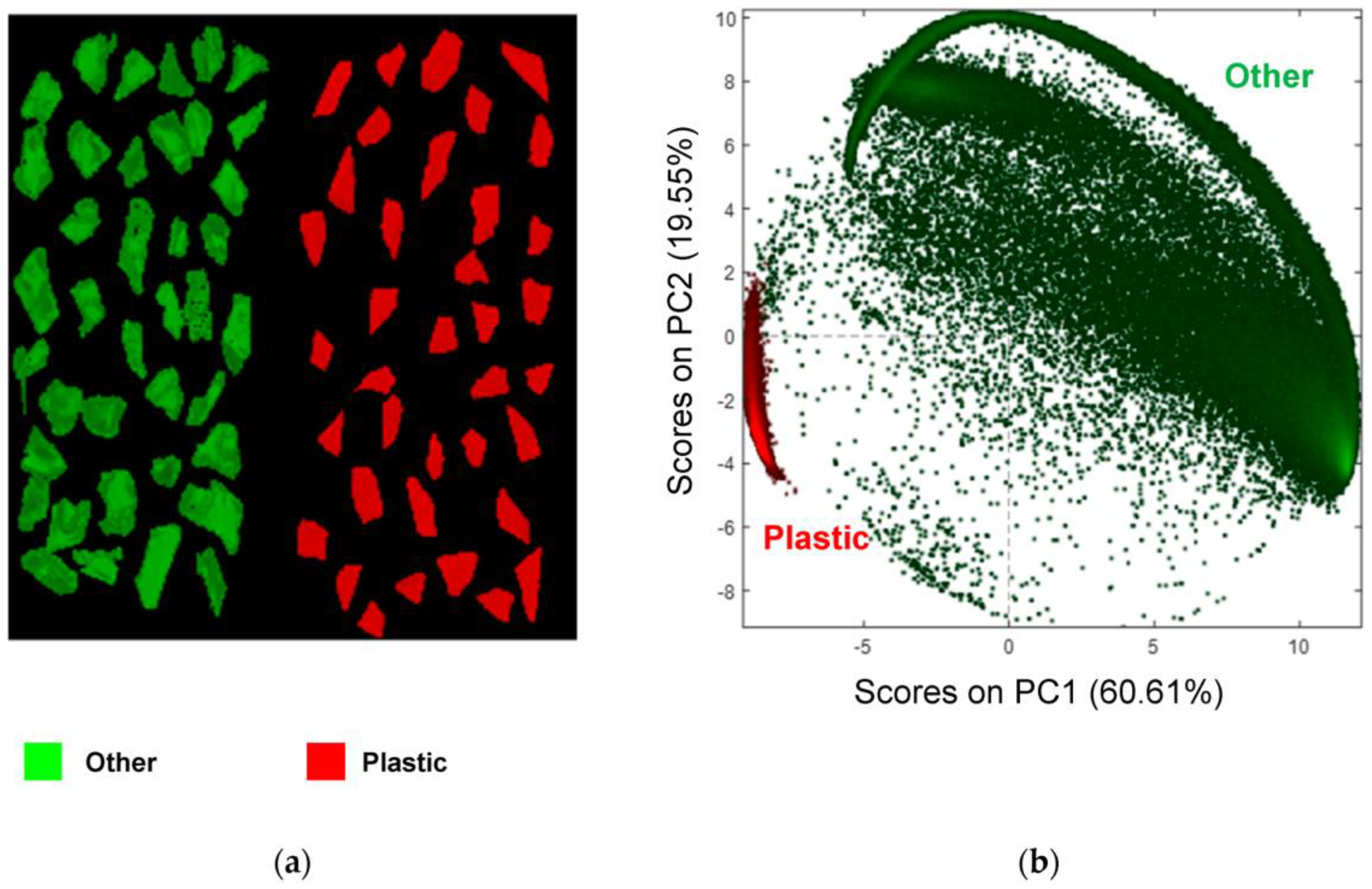
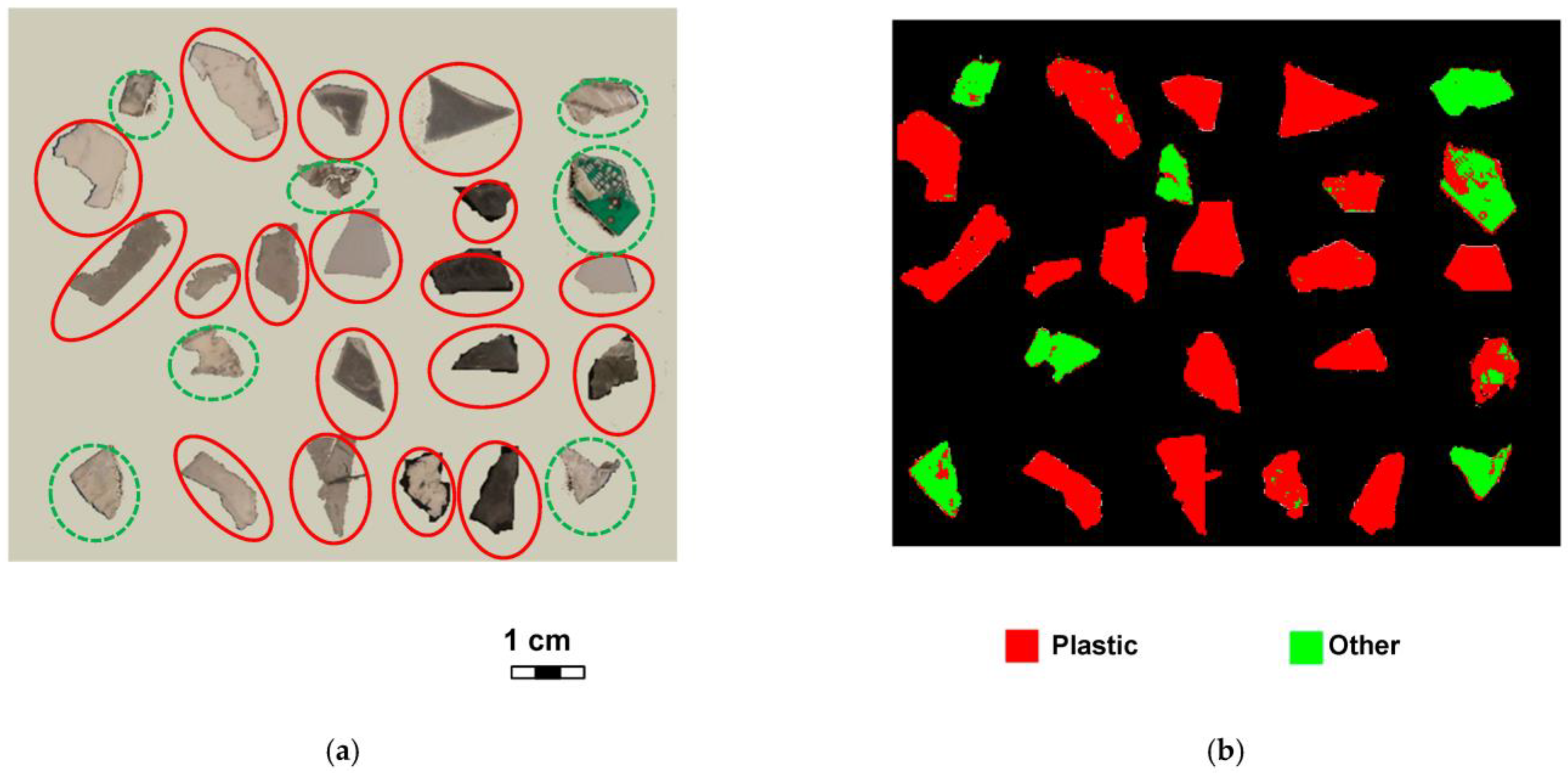
3.1.2. Results of Plastic Flake Identification

The average reflectance spectra before and after preprocessing of the two classes of materials are shown in Figure 2. As can be noted in Figure 2a, the main difference between Plastic and Other raw spectra is found at around 1400–1600 nm, which corresponds to the first overtone combination band of CH [27]. Since most of the Other materials are composed of PCB fragments and various metal particles, it can be assumed that they are inorganic compounds. Nevertheless, the presence of discernible absorptions related to the CH and SH overtones (1700–1750 nm) in the Other spectra suggests the potential existence of organic materials (e.g., cellulose layers or additives) within the investigated samples.
Such a difference is further highlighted by the application of the preprocessing algorithms to the spectra, as shown in Figure 2b.
In Figure 3a, the selected ROIs of Plastic and Other material flakes (training dataset) are shown. In Figure 3b, the obtained PCA score plot of the first two PCs is reported. Most of the variance was captured by the first PC explaining 60.61% of the variance. Classification results in terms of prediction image are reported in Figure 4.
All plastic flakes were correctly identified. The Sensitivity in calibration and cross-validation for the Plastic class reached 0.921 (Table 2), whereas the Sensitivity in calibration and cross-validation for the Other class is 0.813.
In prediction, some misclassified pixels occur for the Other class (Figure 4b). This can be explained by the non-homogeneous nature of the PCB’s surface.

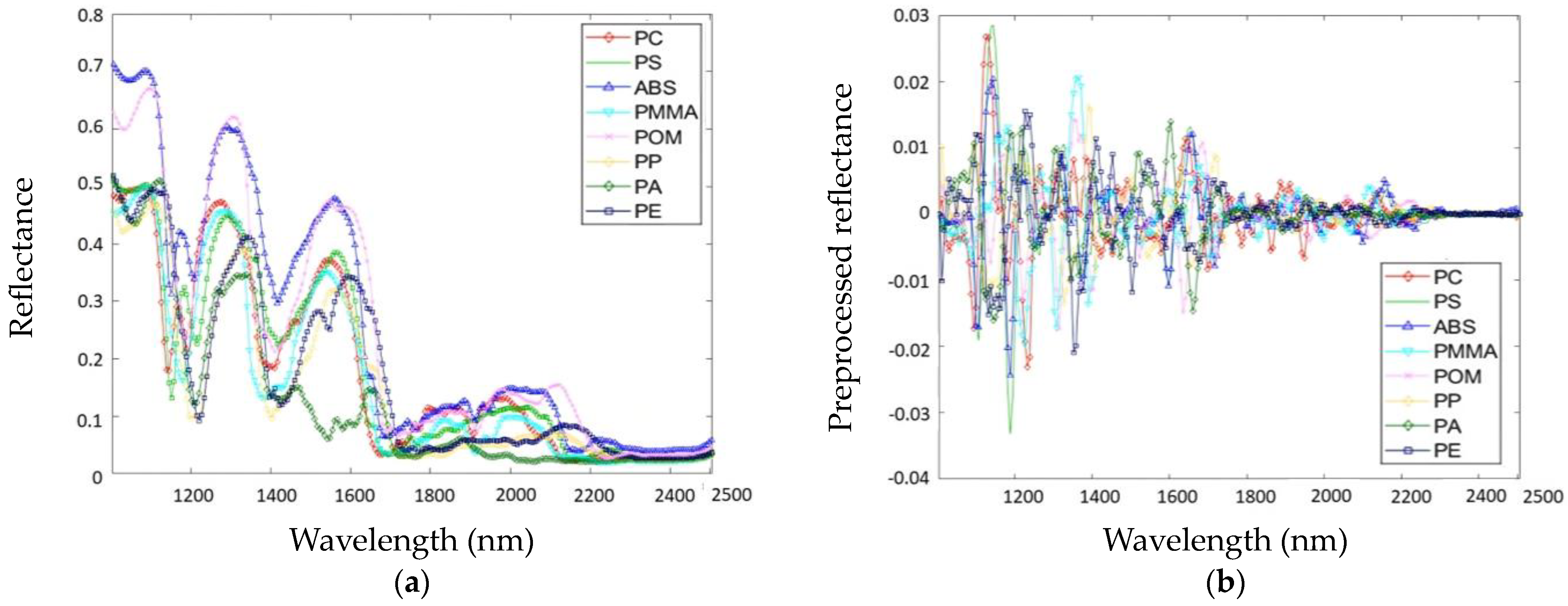
3.2. Polymer Identification Inside a Mixed Plastic Waste Stream Coming from EOL Electronic Devices

3.2.1. Analyzed Samples and Procedure Set-Up

In this case study, plastic flakes resulting from mechanical separation of EOL electronic devices (i.e., housings and trims) were selected in order to build a classification model able to identify the different polymer types for their further recycling in separated streams.
Known virgin polymers were used to build the calibration set, while plastic flakes resulting from the mechanical separation of EOL electronic devices (i.e., housings and trims) were used in the validation set. In more detail, starting from the acquired hyperspectral images of nine different virgin polymers (i.e., PC, PS, ABS, PMMA, PP, PA, PE and POM), preprocessing algorithms were firstly applied. More specifically, Savitzky-Golay (S-G) Smoothing, S-G 2nd Derivative, Normalize and MC algorithms were applied. The S-G algorithm is frequently used to smooth data when taking the derivative, considerably enhancing the usefulness of derivatized data [24]. S-G smoothing fits individual polynomials to windows surrounding each spectrum point. Data are then smoothed using these polynomials. Derivatives tend to amplify noise by de-emphasizing lower frequencies and emphasizing higher frequencies (high-frequency signals).
After that, a PCA model was built to explore the variability of the different polymer spectra. Finally, a PLS-DA was trained using the reference polymer spectra to classify the investigated plastic flakes.

3.2.2. Results of Polymer Identification

In Figure 5, raw and preprocessed spectra related to the virgin spectra are shown.
The SWIR range is a valuable source of information for characterizing polymers due to the absorption of light by overtone or combination bands of carbon-hydrogen (CH) vibrations in their molecules [27].
The analysis of the obtained PCA score plot allows for the identification of pixel grouping according to their spectral signature (Figure 6). The first two PCs captured most of the variance, with PC1 explaining 42.53% and PC2 explaining 29.51% of the total variance. The more the pixels are closer, the more they have similar spectral behavior.
The obtained PLS-DA results, in terms of classification images, are shown in Figure 7, while the corresponding performance parameters are reported in Table 3.
Six polymers in the validation image were correctly detected by the developed PLS-DA model with just a small number of misclassified pixels, mostly due to the border effect. The few incorrectly assigned pixels, however, have little impact on the correctness of classified images. The classification performances revealed Sensitivity and Specificity values in calibration and cross-validation equal to 1.000.

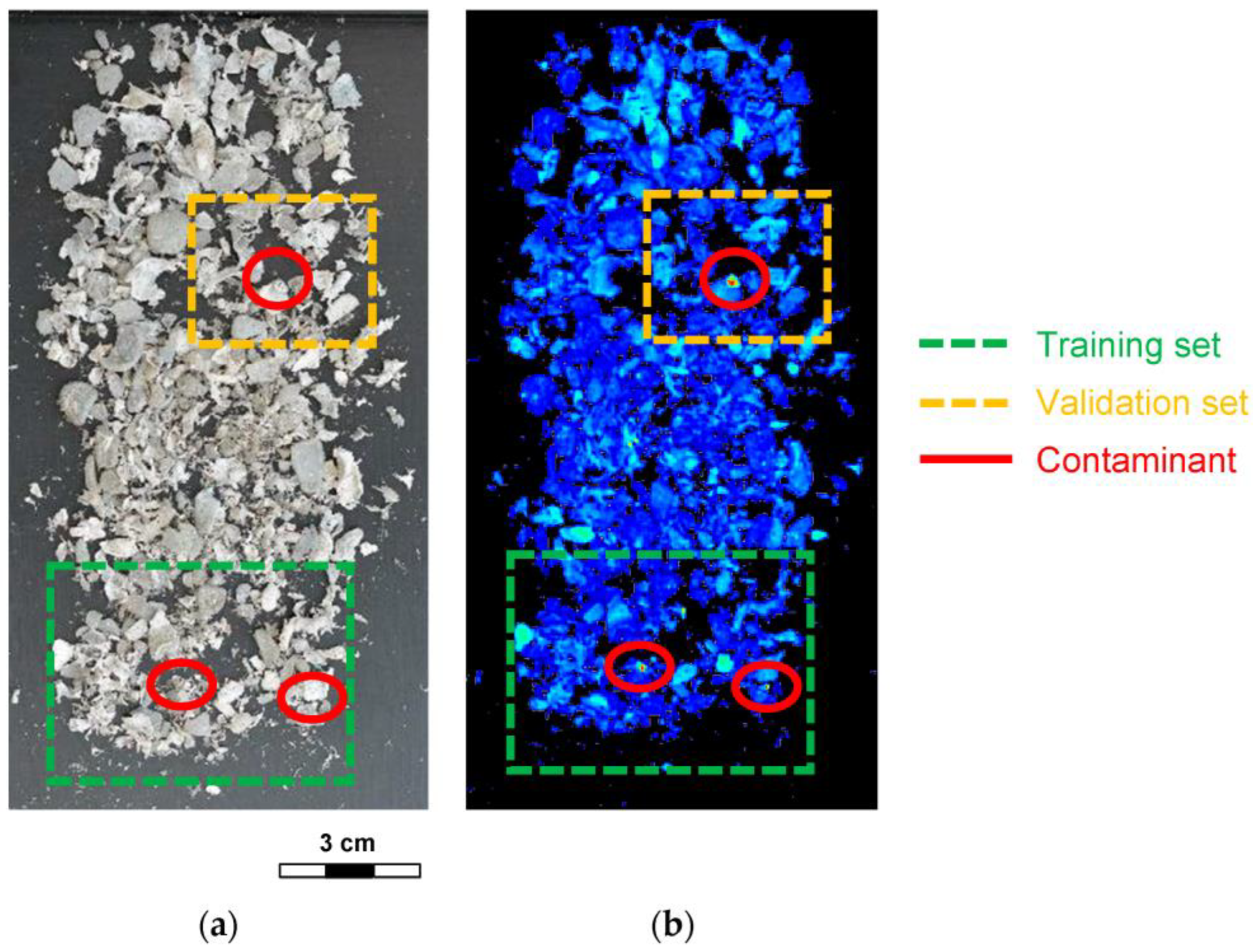
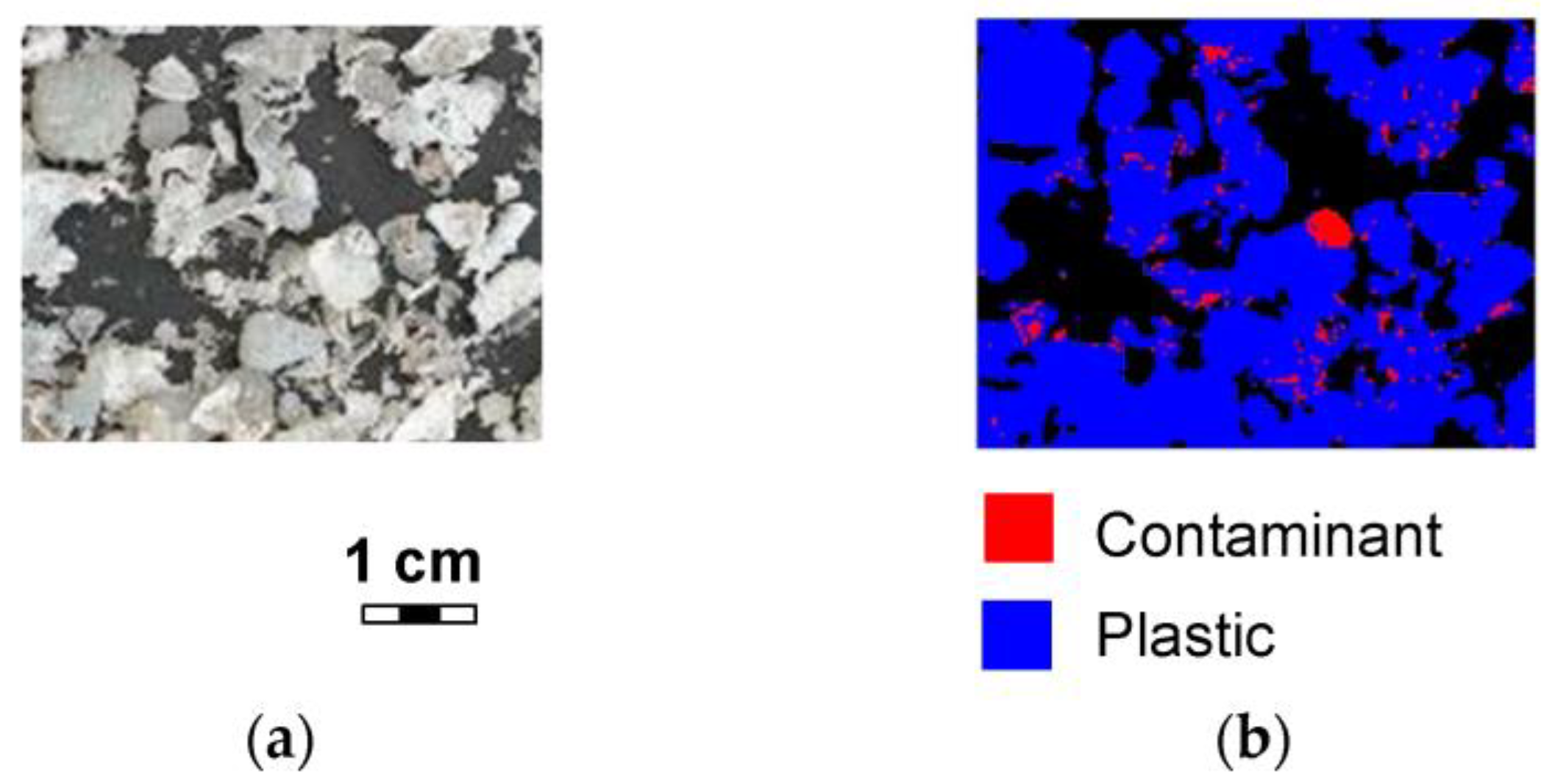
3.3. Contaminant Identification in a Mixed Plastic Waste Stream from the Recycling Line of Electrical Cables

3.3.1. Analyzed Samples and Procedure Set-Up

In this case study, plastic waste particles, resulting from a WEEE treatment plant of electrical cables, were analyzed in order to identify the possible presence of contaminants (i.e., metal particles, such as copper or aluminum) that can negatively affect their further recycling. ROIs were selected from the collected hyperspectral image to obtain a training and validation set (Figure 8).
Plastic and Contaminant classes were assigned to the training set. S-G Smoothing, SNV and MC were chosen for preprocessing purposes. A PCA was performed on the preprocessed hyperspectral image in order to detect and topologically localize metal contaminants. Finally, a PLS-DA was built using the training set and then applied to the validation set, allowing the classification of Plastic and Contaminant classes.

3.3.2. Results of Contaminant Identification

In Figure 8a, the image representing the investigated plastic sample is shown. In the corresponding acquired hyperspectral image (Figure 8b), the presence of metal contaminants is detectable thanks to their ability to reflect more of the source light in comparison to that of plastic particles (Figure 8b). Indeed, red pixels in the hyperspectral image denote spectra with higher average reflectance values. In Figure 9, average raw spectra of the Plastic and Contaminant classes are shown. The Contaminant class shows higher reflectance values than the Plastic class in all the investigated spectral ranges.
As most of the absorption bands seen in the wavelength region 1000–2500 nm are overtones or combination bands of carbon-hydrogen (C-H) vibrations, the investigated NIR range is particularly effective for identifying plastic. Due to their distinctive forms in three wavelength ranges (1150–1250 nm, 1350–1450 nm and 1650–1750 nm), plastic and contaminant spectral fingerprints may be easily distinguished. This is because they have various chemical structures and formulas. The presence of metal contaminants (i.e., aluminum or copper) defines a spectrum with slightly higher reflectance values but distinctive from the plastic spectral signature.
Through the PCA (Figure 10), pixels belonging to the Contaminant class are easily detectable as the related scores in the PCA score plot are far from the Plastic pixel grouping.
The obtained PLS-DA results are shown in Figure 11. Sensitivity and Specificity values in calibration and cross-validation are equal to 1.000 for the Plastic and Contaminant classes. As shown in Figure 11b, the PLS-DA classifier is able to topologically detect the contaminant in the mixed plastic waste stream.

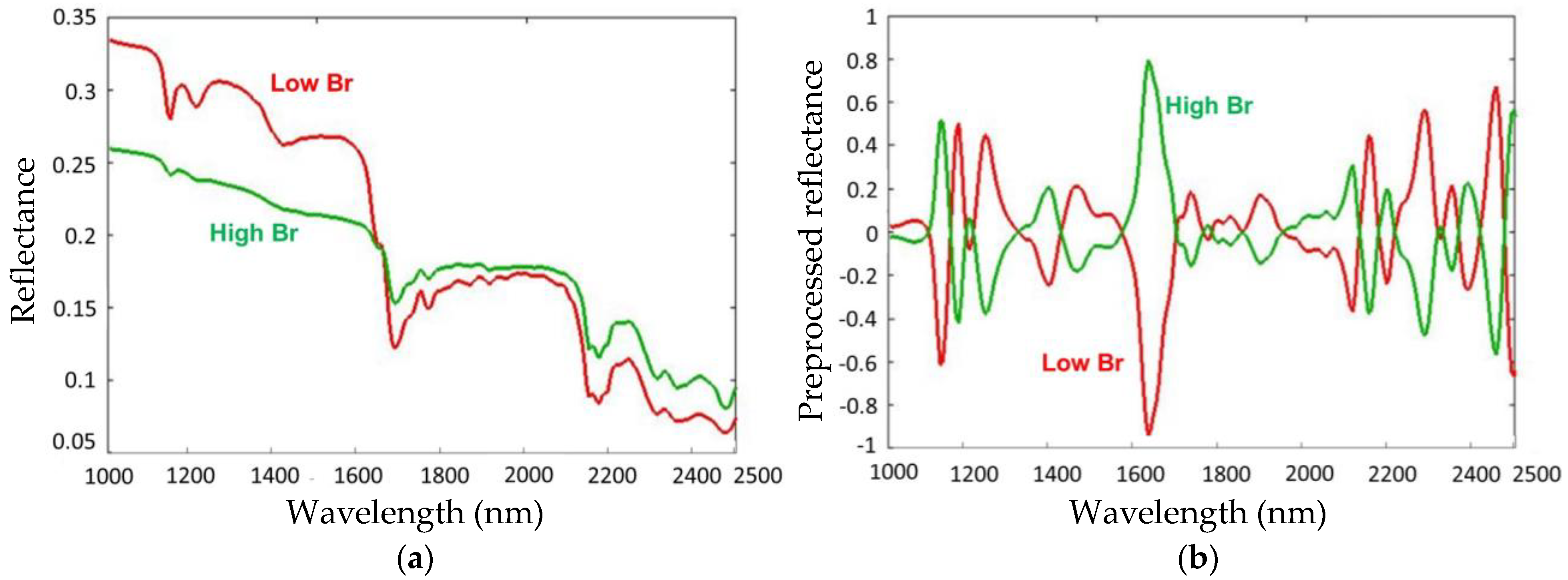
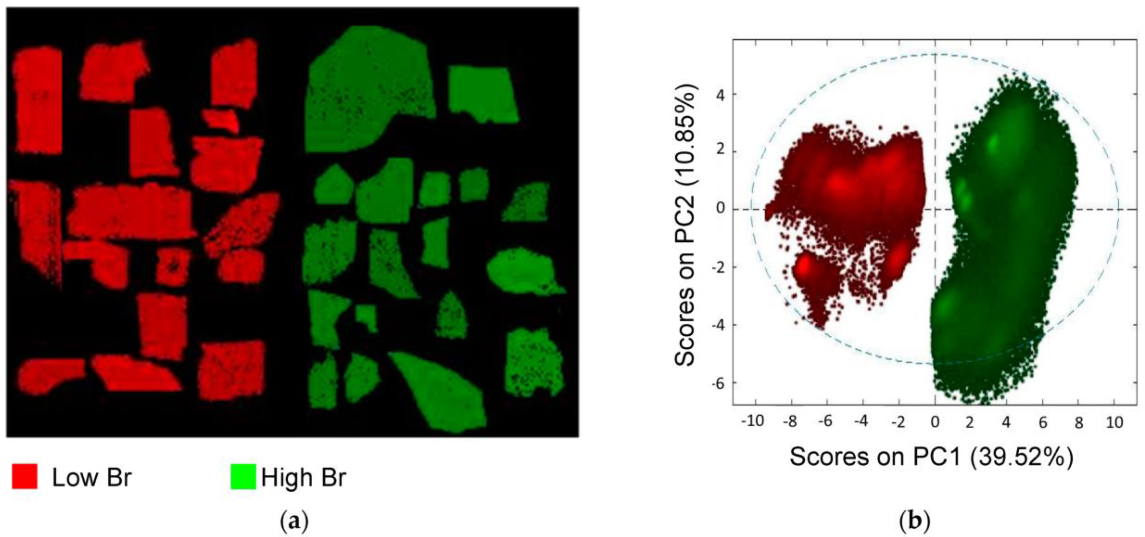
3.4. Identification of WEEE Plastics with Brominated Flame Retardants

3.4.1. Analyzed Samples and Procedure Set-Up

Fragments of plastics waste from small appliances (i.e., cathode-ray tube televisions and monitors) were selected in order to build a classification model capable of recognizing plastics containing quantities of Bromine (i.e., plastic waste containing brominated flame retardants, BFRs) exceeding the limit of 2000 ppm imposed by legislation (CLC/TS 50625-3-1) [21]. These samples were previously analyzed by micro-X-ray fluorescence (micro-XRF) to perform elemental analysis and detect Bromine (Br) concentration. The micro-XRF analysis results regarding the Br content assessment on the validation set used in the HSI procedure are reported in the Supplementary Materials.
This analysis allowed the categorization of the samples into two distinct classes based on their Br content: High Br (Br > 2000 mg/kg) and Low Br (Br < 2000 mg/kg). A PLS-DA classification model was developed to effectively separate the samples into these two classes.
Appropriate preprocessing has been used to correct instrumental noises, scattering effects or any other signal disturbances, but also to enhance the differences between samples. More specifically, S-G 1st Derivative, SNV and MC were applied.

3.4.2. Results of Plastic with Brominated Flame Retardants Identification

In Figure 12, average raw and preprocessed spectra related to the investigated WEEE plastics are shown.
The raw reflectance average spectra of two classes of Br content were analyzed in the SWIR range as it is useful both for identifying the polymer type (harmonic bands of the fundamental groups containing C-H and O-H bonds [28]) and to discriminate samples exceeding the limit of 2000 ppm imposed by the legislation.
Samples with a high Br content, in fact, show an extra absorption peak around 1400–1500 nm and more precisely at 1469 nm. According to previous studies, this peak is due to the presence of tetrabromobisphenol A (TBBPA) [29,30,31]. This difference is highlighted using appropriate preprocessing (Figure 12b).
The analysis of the obtained PCA score plot allows for the identification of pixel groupings according to their Bromine content (Figure 13). PC1 negative values identify the samples with low Br content, while PC1 positive values identify those with high Br content. Most of the variation in the data was accounted for by the first two PCs. In more detail, PC1 explained 39.52% of the variance, while PC2 explained 10.85% of the variance.
The obtained PLS-DA results, in terms of classification images, are shown in Figure 14. The results of the PLS-DA model applied to the validation dataset show that the samples were correctly identified and classified (red: plastic samples with low Br; green: plastic samples with high Br). Sensitivity and Specificity values in calibration and cross-validation are equal to 1.000 for both High Br and Low Br classes.

4. Conclusions and Future Perspectives

The potentialities of the SWIR-HSI system to characterize, inspect and perform quality control or sorting of plastics derived from e-waste solid particles, both during the feeding process and as a result of the different processing activities involved in their recovery.
The results of the investigated case studies demonstrated that the proposed SWIR-HSI approach can be effectively employed: (i) to continuously monitor various streams of plastic waste derived from WEEE prior to or following handling or processing operations, and (ii) to develop new strategies for quality certification and/or sorting applications of waste-derived products.
The presented methodological approach can be seen as a tool to maximize the recyclable polymer fractions by removing contaminants (i.e., metals and plastic waste containing BFRs) and identifying polymer types.
The implementation of this methodology can contribute to the promotion of the principles of a circular economy and achieving the Sustainable Development Goals (SDGs), such as SDG9 (Industry, Innovation, and Infrastructure), SDG12 (Responsible Consumption and Production), SDG13 (Climate Action), SDG14 (Life Below Water) and SDG15 (Life on Land). By improving the circular use of materials, minimizing pollution, toxic emissions and landfills, and also helping to mitigate the impacts on climate change, this approach aligns with the objectives outlined in these SDGs.

Supplementary Materials

The following supporting information can be downloaded at: https://www.mdpi.com/article/10.3390/su151411345/s1, Figure S1. Examples of the micro-XRF distribution maps for Br inside on plastic waste samples; Figure S2. Source images of plastic scraps sample (Low Br and High Br) adopted to define the validation dataset; Table S1: Main characteristics of waste plastics samples with different content of Brominated flame retardant utilized for validation.

Author Contributions

Conceptualization, G.B., S.S. and R.P.; methodology, R.P., L.F. and R.G.; software, R.P., L.F. and R.G.; validation, R.P., G.B., L.F., R.G. and S.S.; formal analysis, L.F., R.G. and R.P.; investigation, G.B., L.F., R.G., R.P. and S.S.; resources, G.B. and S.S.; data curation, L.F., R.G. and R.P.; writing—original draft preparation, R.P., L.F. and R.G.; writing—review and editing, G.B., R.P. and S.S.; visualization, G.B. and S.S.; supervision, G.B. and S.S. All authors have read and agreed to the published version of the manuscript.

Funding

This research received no external funding.

Institutional Review Board Statement

Not applicable.

Informed Consent Statement

Not applicable.

Data Availability Statement

The data presented in this study are available on request from the corresponding authors.

Conflicts of Interest

The authors declare no conflict of interest.

References

  1. Forti, V.; Balde, C.P.; Kuehr, R.; Bel, G. The Global E-Waste Monitor 2020: Quantities, Flows and the Circular Economy Potential. 2020. Available online: https://ewastemonitor.info/wp-content/uploads/2020/11/GEM_2020_def_july1_low.pdf (accessed on 19 July 2023).
  2. Buekens, A.; Yang, J. Recycling of WEEE plastics: A review. J. Mater. Cycles Waste Manag. 2014, 16, 415–434. [Google Scholar] [CrossRef]
  3. Robinson, B.H. E-waste: An assessment of global production and environmental impacts. Sci. Total Environ. 2009, 408, 183–191. [Google Scholar] [CrossRef] [PubMed]
  4. Álvarez-de-los-Mozos, E.; Rentería-Bilbao, A.; Díaz-Martín, F. WEEE recycling and circular economy assisted by collaborative robots. Appl. Sci. 2020, 10, 4800. [Google Scholar] [CrossRef]
  5. Maisel, F.; Chancerel, P.; Dimitrova, G.; Emmerich, J.; Nissen, N.F.; Schneider-Ramelow, M. Preparing WEEE plastics for recycling–How optimal particle sizes in pre-processing can improve the separation efficiency of high quality plastics. Resour. Conserv. Recycl. 2020, 154, 104619. [Google Scholar] [CrossRef]
  6. Chaine, C.; Hursthouse, A.S.; McLean, B.; McLellan, I.; McMahon, B.; McNulty, J.; Miller, J.; Viza, E. Recycling Plastics from WEEE: A Review of the Environmental and Human Health Challenges Associated with Brominated Flame Retardants. Int. J. Environ. Res. Public Health 2022, 19, 766. [Google Scholar] [CrossRef]
  7. Makenji, K.; Savage, M. 10—Mechanical methods of recycling plastics from WEEE. In Waste Electrical and Electronic Equipment (WEEE) Handbook; Goodship, V., Stevels, A., Eds.; Woodhead Publishing: Soston, UK, 2012; pp. 212–238. [Google Scholar] [CrossRef]
  8. Plastics Europe Plastics—The Facts 2022. 2022. Available online: https://plasticseurope.org/wp-content/uploads/2022/10/PE-PLASTICS-THE-FACTS_V7-Tue_19-10-1.pdf (accessed on 19 July 2023).
  9. Calvini, R.; Ulrici, A.; Amigo, J.M. Growing applications of hyperspectral and multispectral imaging. Data Handl. Sci. Technol. 2020, 32, 605–629. [Google Scholar]
  10. Bonifazi, G.; Palmieri, R.; Serranti, S. Short wave infrared hyperspectral imaging for recovered post-consumer single and mixed polymers characterization. In Image Sensors and Imaging Systems 2015; International Society for Optics and Photonics: Bellingham, WA, USA, 2015. [Google Scholar]
  11. Neo, E.R.K.; Yeo, Z.; Low, J.S.C.; Goodship, V.; Debattista, K. A review on chemometric techniques with infrared, Raman and laser-induced breakdown spectroscopy for sorting plastic waste in the recycling industry. Resour. Conserv. Recycl. 2022, 180, 106217. [Google Scholar] [CrossRef]
  12. Zheng, Y.; Bai, J.; Xu, J.; Li, X.; Zhang, Y. A discrimination model in waste plastics sorting using NIR hyperspectral imaging system. Waste Manag. 2018, 72, 87–98. [Google Scholar] [CrossRef]
  13. Bonifazi, G.; Palmieri, R.; Serranti, S. Concrete drill core characterization finalized to optimal dismantling and aggregates recovery. Waste Manag. 2017, 60, 301–310. [Google Scholar] [CrossRef]
  14. Bonifazi, G.; Palmieri, R.; Serranti, S. Hyperspectral imaging applied to end-of-life (EOL) concrete recycling. tm-Tech. Mess. 2015, 82, 616–624. [Google Scholar] [CrossRef] [Green Version]
  15. Bonifazi, G.; Gasbarrone, R.; Palmieri, R.; Serranti, S. Near infrared hyperspectral imaging-based approach for end-of-life flat monitors recycling. At—Automatisierungstechnik 2020, 68, 265–276. [Google Scholar] [CrossRef]
  16. Bonifazi, G.; Gasbarrone, R.; Palmieri, R.; Serranti, S. Hierarchical modelling for recycling-oriented classification of shredded spent flat monitor products based on HyperSpectral Imaging. Detritus 2020, 2020, 122–130. [Google Scholar] [CrossRef]
  17. Geladi, P.; Grahn, H.; Burger, J. Multivariate images, hyperspectral imaging: Background and equipment. In Techniques and Applications of Hyperspectral Image Analysis; Wiley: Hoboken, NJ, USA, 2007; pp. 1–15. [Google Scholar]
  18. Hyvarinen, T.S.; Herrala, E.; Dall’Ava, A. Direct sight imaging spectrograph: A unique add-in component brings spectral imaging to industrial applications. In Digital Solid State Cameras: Designs and Applications; International Society for Optics and Photonics: Bellingham, WA, USA, 1998. [Google Scholar]
  19. Amigo, J.M.; Babamoradi, H.; Elcoroaristizabal, S. Hyperspectral image analysis. A tutorial. Anal. Chim. Acta 2015, 896, 34–51. [Google Scholar] [CrossRef] [PubMed]
  20. Bonifazi, G.; Capobianco, G.; Palmieri, R.; Serranti, S. Hyperspectral imaging applied to the waste recycling sector. Spectrosc. Eur. 2019, 31, 8–11. [Google Scholar] [CrossRef]
  21. Burger, J. Replacement of hyperspectral image bad pixels. NIR News 2009, 20, 19–21. [Google Scholar] [CrossRef]
  22. Burger, J.; Gowen, A. Data handling in hyperspectral image analysis. Chemom. Intell. Lab. Syst. 2011, 108, 13–22. [Google Scholar] [CrossRef]
  23. Wold, S.; Esbensen, K.; Geladi, P. Principal component analysis. Chemom. Intell. Lab. Syst. 1987, 2, 37–52. [Google Scholar] [CrossRef]
  24. Barker, M.; Rayens, W. Partial least squares for discrimination. J. Chemom. J. Chemom. Soc. 2003, 17, 166–173. [Google Scholar] [CrossRef]
  25. Fawcett, T. An introduction to ROC analysis. Pattern Recognit. Lett. 2006, 27, 861–874. [Google Scholar] [CrossRef]
  26. Barnes, R.; Dhanoa, M.S.; Lister, S.J. Standard normal variate transformation and de-trending of near-infrared diffuse reflectance spectra. Appl. Spectrosc. 1989, 43, 772–777. [Google Scholar] [CrossRef]
  27. Weyer, L. Practical Guide to Interpretive Near-Infrared Spectroscopy; CRC Press: Boca Raton, FL, USA, 2007. [Google Scholar]
  28. Workman, J., Jr.; Weyer, L. Practical Guide and Spectral Atlas for Interpretive Near-Infrared Spectroscopy; CRC Press: Boca Raton, FL, USA, 2012. [Google Scholar]
  29. Leitner, R.; McGunnigle, G.; Kraft, M.; De Biasio, M.; Rehrmann, V.; Balthasar, D. Real-time detection of flame-retardant additives in polymers and polymer blends with NIR imaging spectroscopy. In Advanced Environmental, Chemical, and Biological Sensing Technologies VI; International Society for Optics and Photonics: Bellingham, WA, USA, 2009; pp. 114–122. [Google Scholar]
  30. Schlummer, M. Recycling of postindustrial and postconsumer plastics containing flame retardants. In Polymer Green Flame Retardants; Elsevier: Amsterdam, The Netherlands, 2014. [Google Scholar]
  31. Wu, X.; Li, J.; Yao, L.; Xu, Z. Auto-sorting commonly recovered plastics from waste household appliances and electronics using near-infrared spectroscopy. J. Clean. Prod. 2020, 246, 118732. [Google Scholar] [CrossRef]
Figure 1. Methodological approach followed to perform the analysis of hyperspectral images.
Sustainability 15 11345 g001
Figure 2. Average raw (a) and preprocessed reflectance spectra (b) of WEEE shredded flakes.
Sustainability 15 11345 g002
Figure 3. Class setting on the training data set of WEEE shredded flakes (a) and the corresponding PCA score plot (PC1−PC2) (b).
Sustainability 15 11345 g003
Figure 4. Digital image (a) and corresponding false color prediction map obtained by PLS−DA (b) of the investigated mixed WEEE shredded flakes. In (a), red circles with continuous line represent plastic flakes, while other materials are shown with green circles with dashed line.
Sustainability 15 11345 g004
Figure 5. Average raw (a) and preprocessed reflectance spectra (b) of virgin polymers used as reference.
Sustainability 15 11345 g005
Figure 6. PCA score plot (PC1–PC2) of virgin polymer spectral signatures: PC (red diamonds), PS (light green squares), ABS (blue triangles), PMMA (light blue inverted triangles), POM (pink stars), PP (yellow circles), PA (dark green diamonds) and PE (dark blue squares).
Sustainability 15 11345 g006
Figure 7. Digital image (a) and corresponding false color prediction map obtained by PLS-DA (b) of the polymer particles resulting from WEEE mechanical separation operations.
Sustainability 15 11345 g007
Figure 8. Digital (i.e., pictorial) (a) and corresponding hyperspectral image (b) of plastic waste particles, resulting from a WEEE treatment plant of electrical cables.
Sustainability 15 11345 g008
Figure 9. Average raw (a) and preprocessed (b) reflectance spectra of investigated WEEE plastics and detected contaminants.
Sustainability 15 11345 g009
Figure 10. PCA score plot (PC1–PC2) of WEEE plastic and contaminant.
Sustainability 15 11345 g010
Figure 11. Digital image (a) and corresponding false color prediction map obtained by PLS-DA (b) of investigated WEEE plastics and detected contaminants.
Sustainability 15 11345 g011
Figure 12. Average raw (a) and preprocessed reflectance spectra (b) of WEEE plastics with BFRs used as reference.
Sustainability 15 11345 g012
Figure 13. Class setting on the training data set of WEEE plastics with BFRs (a) and corresponding PCA score plot (PC1–PC2) (b).
Sustainability 15 11345 g013
Figure 14. Digital image (a) and corresponding false color prediction map obtained by PLS-DA (b) of WEEE plastics with BFR.
Sustainability 15 11345 g014
Table 1. Different types of polymers and related applications. Adapted from [7].
PolymerTypical Applications
Acrylonitrile styrene acrylonitrile (ASA)Housings, trim
Acrylonitrile butadiene styrene (ABS)Housings, trim
Polymethylmethacrylate (PMMA)Lenses, lighting
Polytetrafluoroethylene (PTFE)Gears, bearings
Liquid crystal polymer (LCP)Coatings, radio frequency (RF) shielding
Polyacetal/acetal (POM)Gears, bearings, insulators
Polyamide/nylon (PA)Structures, clips, casings
Polyamide-imide (PAI)Bearings, insulators, connectors
Polybutylene terephthalate (PBT)Switches, connectors, insulators
Polyethylene terephthalate (PET)Films, screens
Polycarbonate (PC)Screens, casings
Polyethylene (PE)Packaging
Polyetheretherketone (PEEK)Hinges, switches, membranes
Polyetherimide (PEI)Sensors, connectors
Polyphenylene oxide (PPO)Housings, valves
Polyphenylene sulfide (PPS)Connectors, housings
Polypropylene (PP)Packaging, cases
Polystyrene (PS)Housings, trim
Polysulfone (PSU)High temperature applications
Polyurethane (PU)Connectors, coatings
Polyvinyl chloride (PVC)Seals, trim
Styrene/acrylonitrile (SAN)Housings, trim
Table 2. Performance indicators (Sensitivity and Specificity) for PLS-DA classification model, based on HSI acquisition, referred to Plastic and Other classes.
Class:SensitivitySpecificitySensitivitySpecificity
(Calibration)(Calibration)(Cross-Validation)(Cross-Validation)
Plastic0.9210.8130.9210.813
Other0.8130.9210.8130.921
Table 3. Performance indicators (Sensitivity and Specificity) for PLS-DA classification model, based on HSI acquisition, referred to PC, PS, ABS, PMMA, POM, PP, PA and PE classes.
Class:SensitivitySpecificitySensitivitySpecificity
(Calibration)(Calibration)(Cross-Validation)(Cross-Validation)
PC1.0001.0001.0001.000
PS1.0001.0001.0001.000
ABS1.0001.0001.0001.000
PMMA1.0001.0001.0001.000
POM1.0001.0001.0001.000
PP1.0001.0001.0001.000
PA1.0001.0001.0001.000
PE1.0001.0001.0001.000
Disclaimer/Publisher’s Note: The statements, opinions and data contained in all publications are solely those of the individual author(s) and contributor(s) and not of MDPI and/or the editor(s). MDPI and/or the editor(s) disclaim responsibility for any injury to people or property resulting from any ideas, methods, instructions or products referred to in the content.

