1. Introduction
Precision agriculture (PA) is an agricultural management strategy based on data that are collected, processed, analyzed, and combined with other information to drive decisions based on spatial and temporal variability to improve efficiency in the use of resources and the productivity, quality, and profitability of agricultural production [
1,
2].
Although the benefits offered by PA to humankind and the environment are evident [
3,
4], efforts aimed at transforming its general concepts into actions are in progress.
The present article refers to the use of automated and intelligent techniques to recognize vegetable varieties, differentiate cultivation and weeds, and understand how to treat different portions of a cultivated field.
The identification relies on images of vegetation, usually taken from above, that are subsequently processed using specific image analysis and modeling strategies [
5]. This analysis of vegetal covers has been pursued for years for classification purposes, surveys, mapping, biodiversity analysis, and cover dynamics, tasks typically based on remote sensing (satellites, aircrafts) [
6]. However, there are limitations when attempting to perform mapping/classification exercises.
The vegetation canopy is a dynamically structured biological system made of species that strongly interact with one another. Thus, image acquisition and processing are not effortless. Image quality may be influenced by the time at which the image is captured, as well as the height at which it is taken.
More recently, affordable and pervasive technologies such as unmanned aerial vehicles (UAVs) have allowed for images to be captured closer to the ground and at a higher frequency, increasing the acquired details and features [
7].
The increase in picture details and resolution of images from drones suggests the consideration of the possibility of using similar techniques for applications, such as the identification of vegetation patches and weed recognition in variable-rate herbicide spraying (VRHS), the latter being of particular interest in sustainable agricultural applications, as it can aid in ensuring the optimal use of herbicides by reducing unnecessary use [
8,
9]. Benefits offered by the wide use of UAVs, the Internet of Things, big data, and cloud computing from a smart-farming perspective are offered in [
10].
Some weeding machines are already equipped with ground-based cameras for weed recognition, although not fully developed in terms of efficiency [
11]. The environment (lighting sources) and viewpoint (camera positioning) make images considerably different from one another. Surface reflectance and shading are increasingly relevant closer to the surface, making details clearer but also increasing the information to be managed.
The insufficiency of RGB approaches has been recognized by several authors (e.g., [
12]), and many alternative color models have been tested (e.g., [
13]). Alternative color models, such as the HSV (for hue, saturation, value) or HSL (for hue, saturation, lightness), have been developed to simulate color perception systems [
14], distinguishing the hue value from other components related to direct enlightenment and shading (value) or the richness of pigments (saturation) [
15]. Multispectral cameras [
16] were also introduced in experiments to obtain spectrum-related features along with hyperspectral and UV features, the latter of which is aimed at insulating reflectance or induced fluorescence [
17].
However, together with colors, other features can be profitably extracted from an image, some related to regularities (such as patterns) and others that are more noise-like (called texture). While patterns usually scale with distance, texture strongly depends on the resolution, which, in the case of drones, depends on the flight height. Textural features can be approached with structural, statistical, and time-series approaches. A structural approach is similar to pattern recognition, as it refers to repeated/regular regions called texels/textons, while time-series approaches mostly assume picture-wide stationarity/homogeneity, both of which do not fit most landscape images. A series of statistical texture features are described by [
18], offering clear evidence of their use.
A modern and promising approach is based on the ability of machine learning (ML) tools to recognize shapes and structures in a picture due to their ability for ‘pattern recognition’: this is practically done using image embedders properly trained with thousands of images. However, even if the results are sometimes impressive, the availability of a consistent image dataset for training could represent a limiting factor in agriculture [
19]. For example, small variations in crop or weed varieties can produce very different perspectives that are difficult to recognize, not only for an algorithm but also for an experienced farmer.
The present study aims to demonstrate how preliminary aerial-image analysis based on color representations can be combined with low-resource-cost techniques to permit the identification of vegetal species in field crops, especially the recognition of crops from weeds. In particular, it will be shown how an advanced method for color filtering allows for the selection and categorization of a small number of homogeneous image fragments suitable for training several ML classifiers. This is possible due to the use of powerful image
embedders, which can transform pictures into digits while maintaining safe patterns and information. The combination of these approaches allows for us to overcome the limitations of each of them, as well as improve the overall accuracy in vegetable recognition. The outcome of such a hybrid method can be useful in the definition of prescription maps to guide agricultural robots and rovers in their tasks (e.g., weeding, watering, fertilizing). In this sense, the present study is intended to provide an initial guide for the development of robots for laser-based weeding that are currently under investigation [
20] or for similar applications [
21].
2. Materials and Methods
2.1. Investigation Framework
The following steps define the present investigation, as well as the proposed new procedure for providing useful information to drive autonomous robots based on the integration of UAV visible imagery, the HSV model, and machine learning (
Figure 1):
- (a)
aerial reconnaissance with the aim of collecting photographs (‘flat lay’) performed by a commercial drone flying in hover mode at different heights and visual fields;
- (b)
preliminary HSV analysis of images taken from the highest altitude (and largest viewpoint) with the aim of quickly distinguishing characteristic macro areas;
- (c)
preliminary selection of specific sites (inside such macro areas) to be used for training or testing on the basis of crop/weed presence/absence/predominance;
- (d)
image fragmentation into portions (tiles) and their filtering/categorization (by HSV analysis and thresholds) with the aim of building training/testing datasets;
- (e)
use of the training dataset to rank/select the proper image embedders and machine learning (ML) classifiers based on cross-validation procedures and indices;
- (f)
use of the testing dataset to validate the ML accuracy in predictions (species identification) and develop ensemble models for error reduction;
- (g)
use of the new procedure to recognize the crop/weed presence/absence/predominance in all the other field portions, and define overall parameters for quick evaluations.
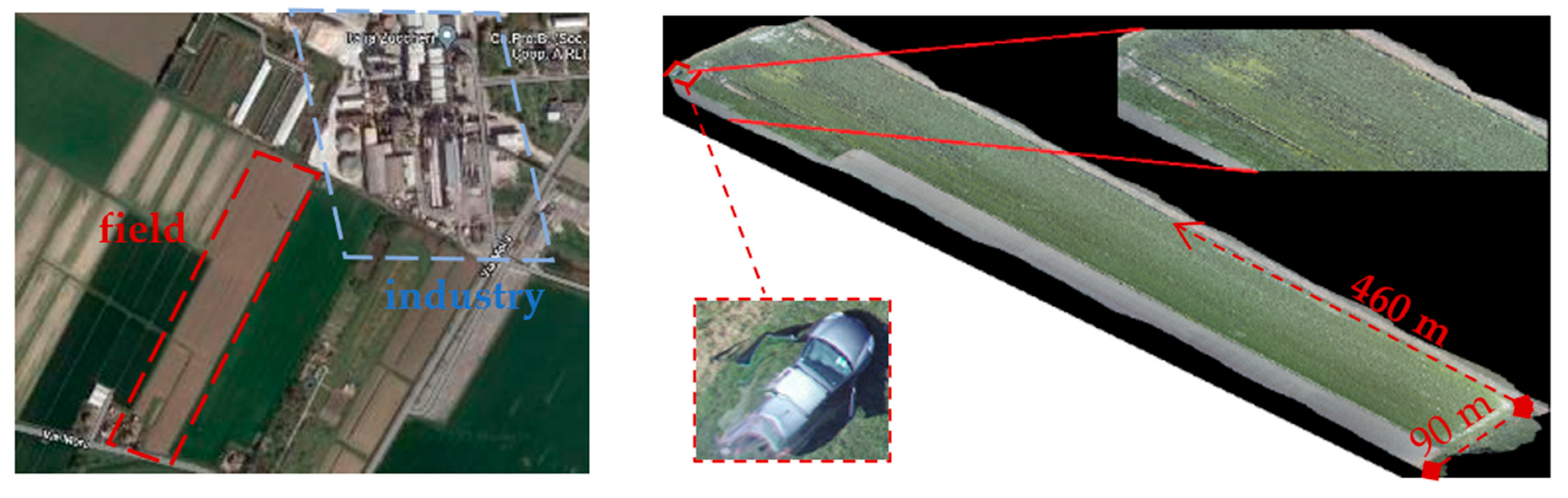
2.2. Experimental Site
The survey was done on a 3-hectare experimental field, ~460 m × 90 m at the largest dimensions, located in Minerbio, North Italy, close to the municipality of Bologna (i.e., lat. 44°37′47.5″ N, long. 11°32′36.6″ E) in late spring (8 May 2020) during the mid-afternoon (3.30–4.30 PM, with a sun azimuth of 259.38° and sun elevation of 35.33°). The field was used for the cultivation of sugar beets, an important crop for the nearby agro-industrial district (
Figure 2), which was left abandoned for several months.
This field, where a well-known commercial crop was obliged to compete with natural species for a long period without external influences, was preferred for its substantial uniqueness. Even if this condition may initially appear to be of little practical use from an ago-economical perspective, it allowed for the evaluation of the efficacy of weed identification in the extreme case of late weeding. Moreover, it permitted the investigation of the ability to identify species in a complex vegetal community that was unexpectedly created.
Weeds are able to outcompete sugar beets for vital resources (solar radiation, water, and nutrients) that are required for optimal production. Infestation significantly affects the productivity of the crop: according to an internal estimate, for every 1000 kg/ha of weeds, there is a reduction of 27 kg/ha of sucrose.
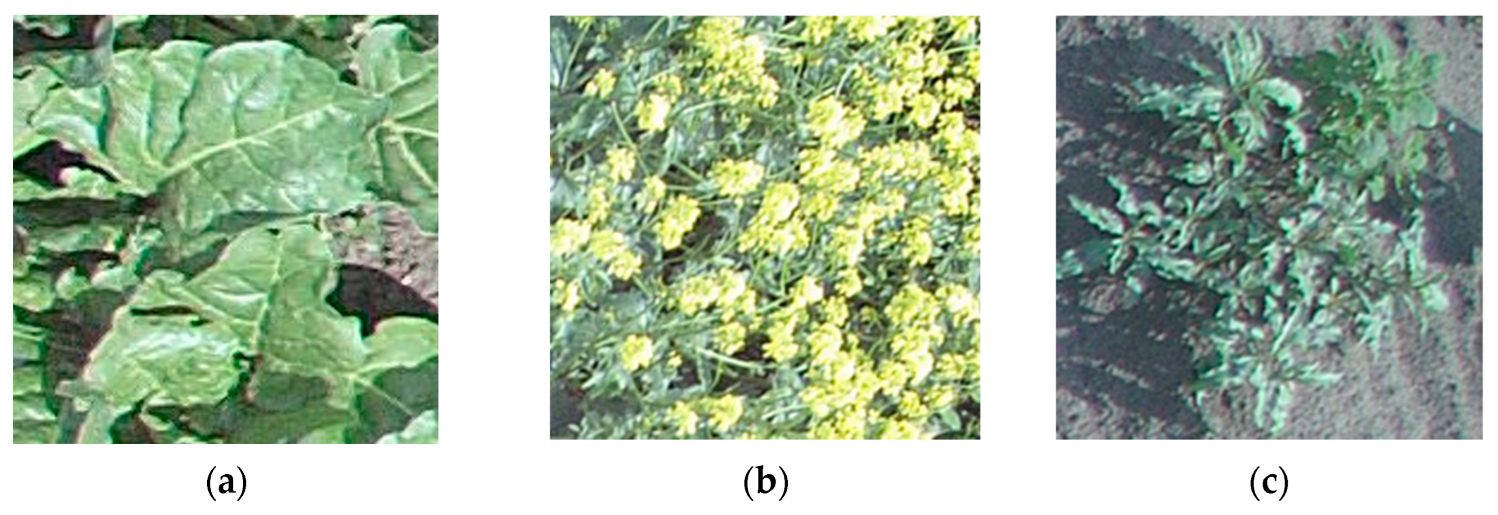
The selected field, rain-fed (no irrigation) and untreated (no herbicides), grown with sugar beet (i.e.,
Beta vulgaris var.
saccharifera), revealed large patches of
Sinapis arvensis and
Chenopodium album, two typical weeds of this part of the Mediterranean area (
Figure 3). The presence of a yellow bloom is also evident for
S. arvensis.
2.3. Aerial Reconnaissance
A commercial drone, mod.
Yuneec Typhoon H, a hexacopter weighing 1.9 kg ([
22]), equipped with a digital camera, was used to take pictures at different altitudes (5, 7, 15, and 35 m), with a 120° lens angle and 4K/DCI resolution (4096 × 2160 pixels). The flight lasted almost 20 min, and 320 photographs were taken in total. The specific altitude influenced the width of the field of the photos, which varied from approx. 80 to 4000 m
2. The altitude also influenced the picture resolution, which ranged between 45 and 325 pixels per meter (PPM), equivalent to a discretization of 10 to 0.2 digital pixels per square centimeter: these values represent the size of the smallest detail that could be recognized in each photo (
Table 1). Lower altitudes would certainly increase the image resolution and, perhaps, the recognition efficacy. On the other hand, they would increase the flyover time, the number of photos taken, and the complexity in the elaboration. The optimal choice depends on several factors, including the experimental methods and equipment, environmental conditions, and vegetables, as well as the research scope. However, past investigations suggested similar altitudes, ranging from 3 m above the canopy in the case of structural studies [
23] to 25 m in the case of UAVs equipped with high-resolution multispectral cameras [
24].
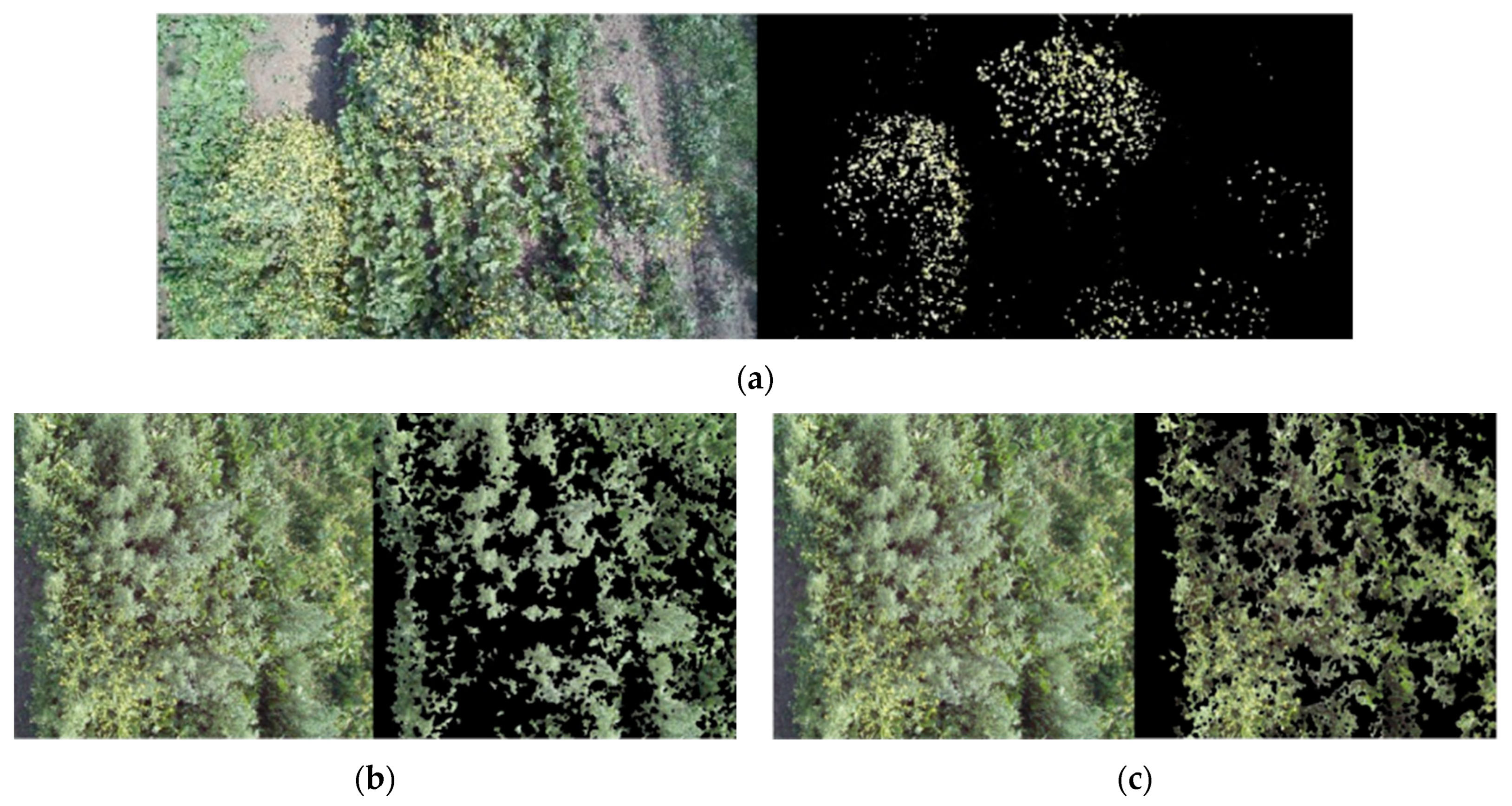
In
Figure 4, images from the two extreme flight heights (35 and 5 m) are shown. From 35 m (
Figure 4a), large patches of
S. arvensis (yellowish middle bottom region) and
C. album (bluish middle top region) were recognizable in the sugar beet field. Going down to 5 m, it is evident how weeds were interspersed with the crop and how the field also included several totally degraded areas. It is also evident how yellow and blue shades could roughly represent the two weeds for an initial classification of species.
The comparison in
Figure 4 also emphasizes the need to detect photos from varying heights when addressing different purposes. Specifically:
Wide photos, taken from 35 m, characterized by lower resolution, were used to identify and select two homogeneous zones inside a quite inhomogeneous moderately sized cultivation field, with the specific aims of training and testing the ML algorithms;
Narrow photos, taken from 5 m, were used to investigate these sites at higher resolution. Homogenous spots (i.e., tiles of 84 × 84 pixels each, approx. 100 × 100 mm) were identified and used to detect (by color-based image analysis) the prevalence of one of the four elements: B. vulgaris, C. album, S. arvensis, and bare soil.
Two sites, namely,
Site A and
Site B, were selected considering aspects related to the presence and spatial distribution of weeds. Photos of the sites are shown in
Figure 5. With a weed prevalence of 39.5% and 57.7% (as evaluated below), these sites were selected to train and test the ML method, respectively. With a lower weed prevalence, also distributed in distinguished zones allowing for a better categorization of images,
Site A was preferred to derive a clear training image dataset. In contrast,
Site B, with opposite characteristics (higher weed prevalence), was considered a better site to test the method potentialities.
2.4. Color-Based Image Analysis
Image analysis and transformation were implemented using the Image Processing Toolbox routines embedded in MATLAB (ver. 2020a, MathWorks) with the aim of:
converting pictures from RGB to HSV color space;
extracting the hue component (H) as a grayscale image;
identifying hue thresholds from uniform surface spots;
identifying texture features;
providing a smooth contour from pixel-based segmentation;
Computing ratios of the segmented area to reference masks and with respect to the total area.
Specifically, in the aerial photos of
Sites A and
B (
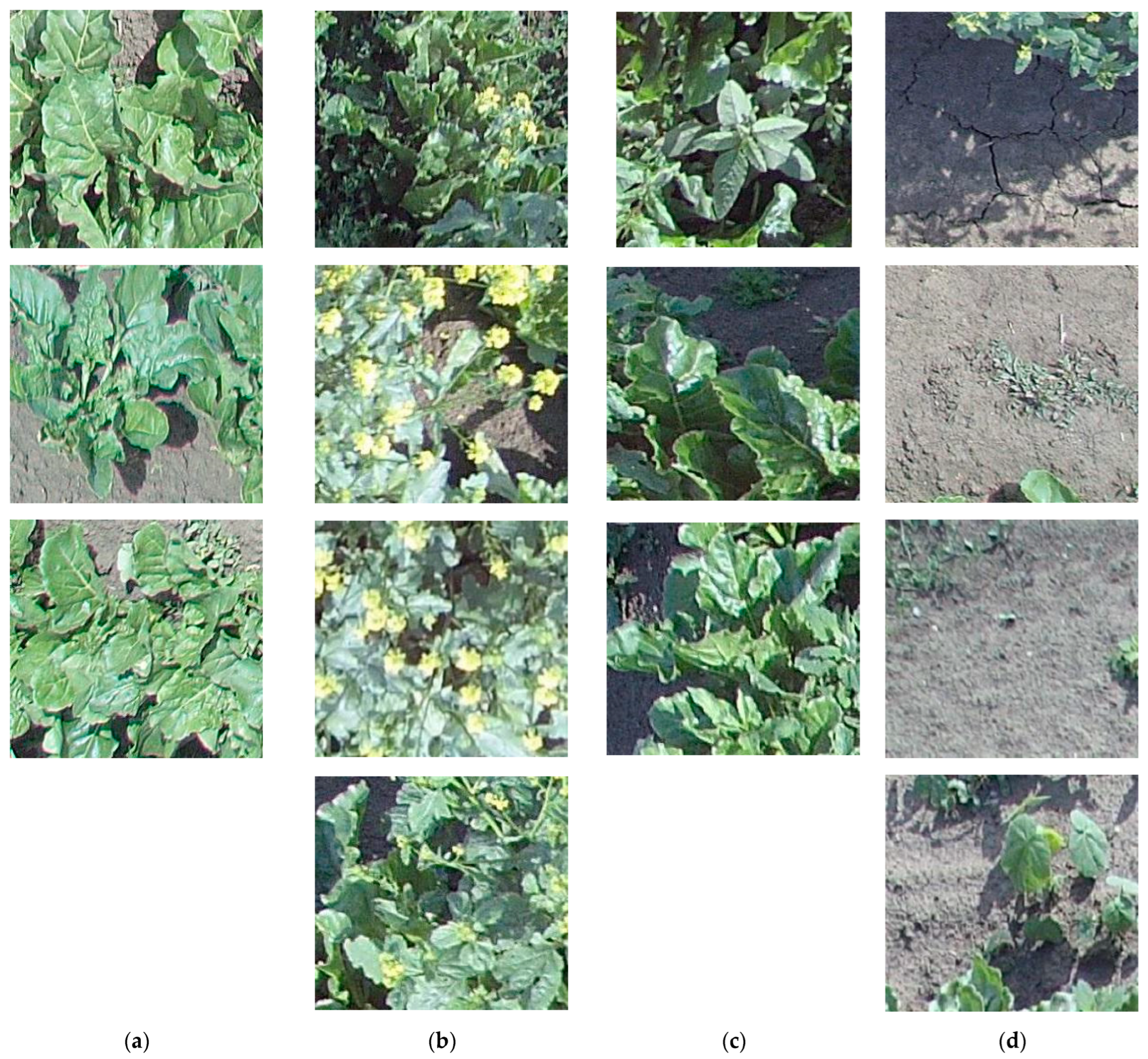
Figure 5), four specific spots characterized by the clear exclusive presence of only one of the four elements (i.e., bare soil,
B. vulgaris,
C. album,
S. arvensis) were first selected (
Table 2), and hue spectra were detected.
The crop hue ranged between 50 and 130, with a predominance in the 65–115 interval.
C. album’s spectrum had more bluish hues, ranging between 65 and 180, and most of the values were below 100.
S. arvensis hues were typically spread between 65–115, with values up to 160. However, since
S. arvensis was in bloom, two discontinuous ranges were clearly detected at 50–100 (with flowers) and 90–140 (without flowers). Similarly, the soil hue had two ranges of hue values, opposites in the scale of values considered, between 10 and 60 in light and between 200 and 270 in shadow. Hue (H) value bars are shown in
Figure 6.
Overlaps between typical hue ranges were evident, especially between
B. vulgaris and
C. album, making it difficult to identify varieties using the HSV method alone, reaffirming the need to integrate a color-based method with a different approach. This is also evident in
Figure 7, where the characteristic hue ranges were applied to pictures showing how
B. vulgaris cannot be easily distinguished (as in the case of
S. arvensis).
Due to such important superimposition, the hue was not used here to detect species (as, e.g., in [
25]), but instead to support the preparation of a training dataset. This was possible by identifying proper thresholds to differentiate the characteristic spectra (everything in between was discarded). As a result, the dataset comprised a smaller number of images, but all of them were clearly defined in terms of characteristics.
Specifically, the photos of
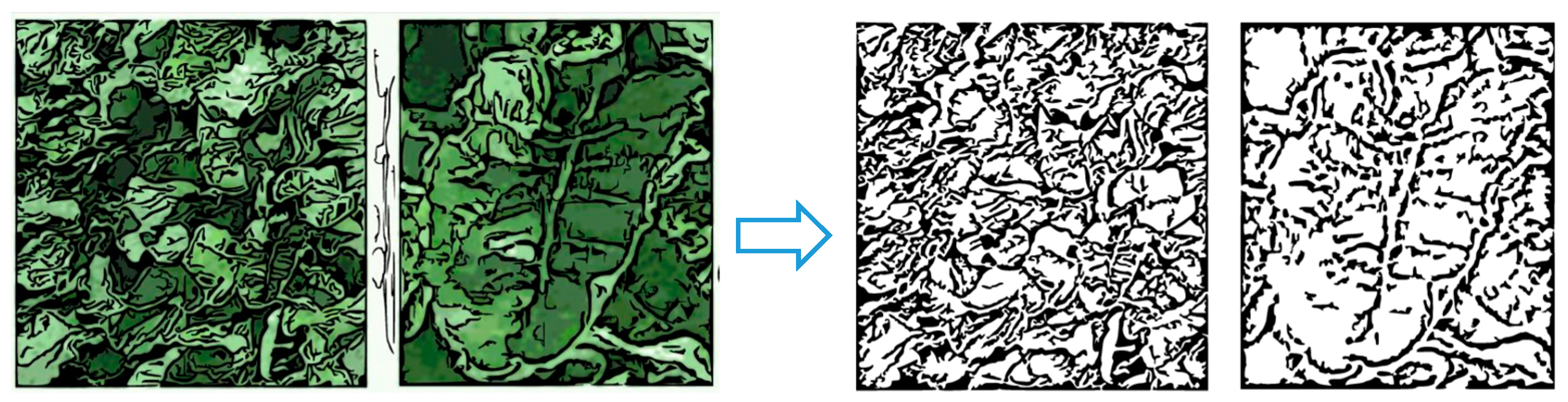
Site A were processed according to the new hue ranges to extract texture. Masks were used for a preliminary identification of the hue intervals. An unsupervised texture segmentation approach using Gabor filters (as in [
26]) was applied. The images were converted to HSV images, and the hue channel was used to reduce the effects of shading and lighting intensity. Dotted results were successively applied using a flood-filling procedure in a way that can be easily automated ([
27]). This process of filtering was applied together with an additional process of partitioning with the aim of providing a convenient number of individual subimages.
2.5. Image Partitioning
The original images were divided into square tiles of different dimensions. Whenever information detected between the tiles showed an overlap in characteristic ranges over a threshold (e.g., 30%), it was excluded to assure a net separation. This approach, based on the preliminary hue analysis of
Site A, allowed for the enhancement of the subdivision in schematic portions (as shown in
Figure 8) for an approach achieved by layering contour masks and weighted overlaps (
Figure 9).
Partitioning aimed to create small groups of subimages, dividing them into homogeneous categories. In the present analysis, four categories were used: B. vulgaris, C. album, S. arvensis, and soil.
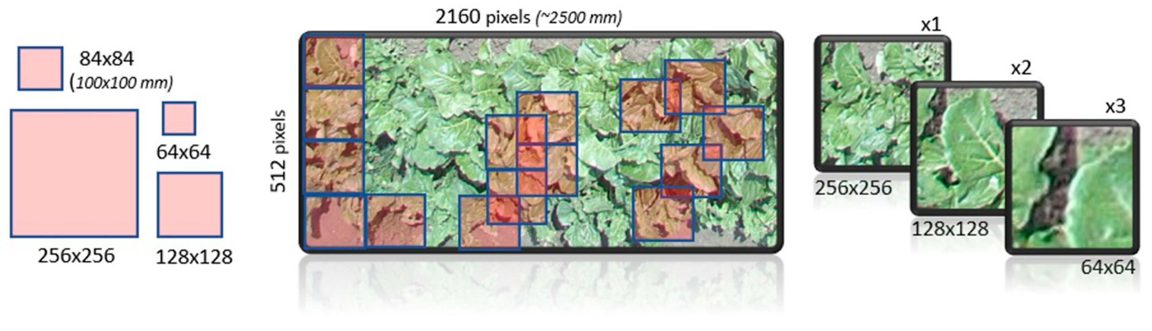
The homogenization also had to consider aspects related to the position of the extraction and size of tiles. Different alternatives were considered as tile sizes: three on a pixel basis (64 × 64, 128 × 128, 256 × 126) and one real size of 100 × 100 mm (84 × 84 pixels). These tiles were taken by splitting the original photos into side-by-side frames. An alternative spatial arrangement, based on partial frame superposition, would have allowed for an increase in the number of extracted images (this maneuver was not necessary, however, since the results were already excellent without overlapping) (
Figure 10).
Several image datasets were built and are summarized in
Table 3.
2.6. Machine Learning
Orange ver. 3.30 platform, an open-source machine learning (ML) toolkit developed by the University of Ljubljana [
28,
29], was used to perform data analysis and visualization, as it provides powerful tools for data classification, clustering, cross-validation and prediction, as well as several useful functions for image analytics. This platform has been applied in many areas of science and engineering, including agriculture [
30].
In this study, a convenient workflow for image analysis and data mining was developed based on a few relevant aspects.
2.6.1. Target Category
First, it was necessary to select the purpose (target) of the analysis to accept the decision effects in terms of the output types and prediction accuracy. Two alternative approaches were considered here based on the way the images from the training dataset were categorized.
In the first case, images were classified considering each of four categories (i.e., B. vulgaris, C. album, S. arvensis and soil). In the second case, a binary classification was performed to distinguish the presence or absence of B. vulgaris. For this purpose, all classes that were not B. vulgaris were grouped together as a single category before training.
Although this second approach seems to offer less information (as it does not allow for distinguishing between C. album, S. arvensis, and soil), it was expected to improve the accuracy in prediction due to the larger number of images the ML algorithms could be based on. Furthermore, such binary information could frequently be sufficient for the scope to know how to proceed (i.e., deciding whether to water or apply an herbicide).
2.6.2. Image Embedding
First, images were converted into numeric vectors using deep learning algorithms to transform each image into its representative features. They returned an enhanced data table with image descriptors that allowed for moving the data mining from images to numbers. Several embedders were available in Orange (e.g.,
Inception by Google,
VGG-16 and
VGG-19 or
DeepLoc) and compared, and the best result was obtained by the so-called
Painters embedder. As it contains ML algorithms that can decompose the image into 2048 numerical features, the embedder was originally trained on 79,433 images of paintings by 1584 painters with the aim of properly predicting painters from artwork images. This general characteristic also pairs with the evidence that tiles from different categories (as shown in
Table 2) mostly looked like paintings painted by different painters.
A data table consisting of 2048 features per image was created, with the number of images depending on the specific dataset under consideration (as in
Table 3). A reduction was also implemented via principal component analysis (PCA), which is a process of computing the principal components and using them to perform a change of basis on the data, sometimes using only the first few principal components and ignoring the rest. Nonrepresentative features were ignored, and the new data table was restricted to 100 features, which were still able to identify the entire dataset.
2.6.3. Hierarchical Clustering
A preliminary analysis was performed on images in terms of distance. It aimed to group the images into clusters based on their similarities (i.e., hierarchical clustering) by evaluating the distance between their representative vectors (as determined by the image embedding process). Such a distance can be weighed by different metrics; the Euclidean metric (i.e., total distance as the square root of the sums of the squares of the distances of each vector component) is the best known. However, the cosine metric was preferred here.
This metric, which evaluates the cosine of the distance between two vectors of an inner product space, allowed for the minimization of distortions related to the scale in the case of images. This means that similar images are clustered regardless of the zoom.
Hierarchical clustering by distance metrics was used here for two reasons:
This means that hierarchical clustering allowed for us to preliminarily assess the ‘goodness’ of information inside datasets to: (i) verify any initial errors in categorization; (ii) exclude uncertain cases (outliers), allowing for a better machine learning process; and (iii) evaluate the prediction accuracy.
Finally, the adoption of a distance metric also allowed for us to search for the elements in the dataset closest to a given element with the aim of understanding the proper category to better allocate such new elements. In this way, the distance itself can be considered a classifier, as it allowed for data classification into groups, but is not considered a learner, as it does not learn anything from information. These differences are explained below.
2.6.4. Classification Models
The study considered 6 of the most common ML algorithms:
Logistic regression (LR);
k-Nearest neighbors (kNN);
Classification/Decision tree (CT);
Random forest (RF);
Neural network (NN);
Support vector machine (SVM).
The above are supervised ML algorithms that are able to operate as classification tools according to different logics: their simultaneous use provided additional information and better predictions. A short overview and comparison of the algorithms are available in [
31,
32,
33] and offer a wider perspective.
Although it would be relatively easy to include additional models (e.g., logistic regression, naïve Bayesian) in the analysis, no added value was evident since good predictions were achieved without them. The accuracy was evaluated considering all available criteria to score/rank each classifier (e.g., R-squared, RMSE, MAE). Specifically, even if all criteria were kept under control to prevent misinterpretations, the final assessment was made in terms of ‘Precision’, defined as the proportion of true positives among instances classified as positive. This criterion was preferred because it can provide a normalized and immediately understandable index.
2.6.5. Learner Test and Score
Notably, there is no a priori method to determine the best model(s) with respect to a given dataset [
34,
35]. A standard approach for the scope consists of using part of the dataset to validate and test the algorithms. Then, the dataset is typically divided into three parts to be applied for training, validation, and testing (
Figure 11).
Representatives of each group are randomly selected from the original dataset, paying special attention to their size. The larger the sample used for validation or testing, the less data are available for training, making it difficult for learners to learn and predict. Conversely, the smaller the sample used for validation or testing, the greater the risk of extracting nonrepresentative elements. To ensure statistical consistency, the procedure must be replicated several times, averaging the outputs.
The same approach was applied here with minimal changes to investigate different validation/test scenarios. During validation, the largest part of the tiles (80–95%) was used for training, while the remaining tiles (5–20%) were used for validation. These sizes were modified to investigate their effects on the output.
An acceptable procedure for validation consisted of using 80% of images for training and 20% for validation; then they were ‘stratified’ to account for the consistency of different subpopulations and replicated 10 times. However, perhaps the best compromise between the execution speed and accuracy in prediction was offered by 90%/10% datasets, repeated 20 times.
No significant change in the accuracy was observed when a cross-validation procedure was performed, which is a resampling method that uses different portions of the same data to test and train a model on different iterations.
To check such a consideration, the so-called ‘leave-one-out’ approach was used, which holds out one instance at a time, inducing the model from the remainder and then classifying the held-out instances. Such a method, which is very stable and reliable, although slow, did not introduce significant changes in the output (i.e., learners’ rank).
Finally, in the case of the test, 90% of the images were used to populate the training dataset and 10% were used for the test dataset. These images were randomly extracted from the original dataset and were categorized manually (not through the hue-based procedure).
3. Results
Although different combinations were investigated and compared, the results herein mainly refer to dataset
c (see
Table 3), consisting of a small number (140) of large tiles (256 × 256 pixels, ~104 mm
2) derived from one aerial photo of
Site A (as shown in
Figure 5a), which was fragmented and categorized by hue-based image analysis (which also discarded the uncategorizable tiles). Specifically, the presence of
B. vulgaris was detected in 23 tiles;
S. arvensis was detected in 56 tiles;
C. album was detected in 26 tiles, and bare soil was detected in the other 35 tiles.
3.1. Neighbors
Based on the cosine distance, hierarchical clustering was performed first. With respect to a maximum depth of 10 levels, the 23 tiles of B. vulgaris were always classified in the same group, sharply separated by others. This suggests an excellent clustering of the training data.
Figure 12 shows an example of how to interpret the concept of
neighborhood between images by showing representative images at an increasing distance from the selected image.
It can be seen that very close images to the reference image of a sugar beet are almost indistinguishable, with minimal differences in the shape and thickening of leaves. Moving away toward the extreme of the sugar beet group, the images are more differentiated. For instance, leaves are more scattered, and visible areas of soil emerge. Moving further away, the first elements of other categories become apparent. Specifically, it is evident that C. album is not so different from the starting image because C. album and B. vulgaris are intertwined in cultivation in such areas. Moving significantly away, another category emerges in photos containing a significant presence of bare soil. These photos suggest that B. vulgaris is rarer. Finally, in the last category, S. arvensis is clearly different in terms of the shape, size and color.
Thus, everything appears correct in this preliminary clustering, especially when focused on B. vulgaris. At a deeper level of detail (as done later), some overlapping areas between S. arvensis and C. album or between C. album and bare soil are evident.
3.2. Learner Selection and Validation
Orange implements a feasible tool to test and score learners (i.e., ‘
Test and Score’) that permits the quick modification of criteria and parameters. In the stratified case of 90% of data used for training and 10% used for testing, it reported a very high precision over the classes. When measured as the area under ROC curve (AUC), LR scored 0.991, higher than NN (0.983), SVM (0.976), and slightly less than others, while the CT accuracy was significantly lower (0.796). Nothing truly changes if other evaluation criteria (such as the classification accuracy, F1, recall, etc.) are preferred, with minimal differences in ranking. When the precision is focused on
B. vulgaris as the target class, all five classifiers (excluding CT) offer 100% accuracy, confirming the value of the procedure (
Table 4).
Using a confusion matrix, it is possible to define the risk that a prediction is right or wrong with respect to each classifier.
Table 5 reports the confusion matrix for the very effective NN and RF classifiers, as well as the worse-performing CT. It is evident that NN and RF never result in confusion in the case of sugar beet, correctly predicting it in 100% of cases (unlike the CT that gets it right 68.2% of the time). Bare soil was also easily recognized by the NN and RF (93.9% accuracy), while the remaining cases (6%) were considered synapsis by the RF and were not distinguished by the NN. Furthermore, NN and RF showed a certain difficulty (between 11.5% and 23.8%) in recognizing
C. album, with NN weaker on
S. arvensis and vice versa. However, this lack of precision could not depend on the learners when it can be traced back to an imperfect clustering of the starting information, which is also evident from the previous hierarchical clustering analysis. An improvement could be achieved by the better filtering and classification of the images.
3.3. Direct Validation
A second validation on
Site A was carried out by extracting a small number of items and checking them. This procedure was manually implemented to have total control over the test case. Specifically, 14 photos from the 4 categories of
B. vulgaris (3),
S. arvensis (4),
C. album (3), and soil (4) were randomly extracted from the dataset and used for comparison (
Figure 13). Before any other consideration, it should be noted that the 14 photos represent a nonnegligible amount (10%) with respect to the whole dataset consistency (140): their extraction weakens the training process and impacts the overall accuracy. In this regard, it should also be remarked that cross-validation identifies one single item (instead of 14) for the extraction at a time. Thus, the training dataset remains almost complete.
As expected, the accuracy slightly dropped: the AUC ranks SVM (0.993), LR (0.986), kNN (0.976), NN (0.973) RF (0.908), and CT (0.767), confirming the learners’ ability to offer valid predictions even in the case of a 10% reduction in training data.
Finally, it was also possible to verify the prediction offered by each classifier with respect to all 14 testing photos. Some of them are shown in
Table 6, where the actual and predicted categorization in terms of probability is reported. For instance, in the case of the first row, the LR classifier correctly predicted
B. vulgaris and bare soil, with a probability of 99%. Then, it suggests considering the third image, initially clustered as
S. arvensis, soil, since the probability of correspondence with
S. arvensis is approximately 29% (with a probability of 71%). Similarly, it suggests considering the fourth image as
S. arvensis instead of
C. album, although in this case the difference in probability is marginal (53% vs. 47%).
The results show how learners were very accurate, and the faults with respect to conditions were rather difficult to interpret (e.g., shadows). For instance, in addition to the accurate recognition of the sugar beet in almost all cases, learners correctly identified (78–100%) the soil even when shadows and traces of S. arvensis might have been confusing. They even found a mismatch with respect to the initial cataloging in the case of the third tile, incorrectly entitled S. arvensis due to some small flowers shining under the direct sun against the dark soil. All classifiers ignored such disturbing factors and recognized the potential misclassification, suggesting the presence of soil.
Finally, the fourth photo was the most uncertain even for human experts due to the contents of the photo, where the presence of C. album can be observed against a background of B. vulgaris. With respect to this, each classifier offered a different answer based on its peculiarities. For example, the TR that works on multiple image levels recognized (100%) and highlighted the presence of B. vulgaris, which is predominant, masking C. album. The other 4 learners confirmed the original classification by identifying such a situation as similar to others in which they noticed C. album infesting the substrate.
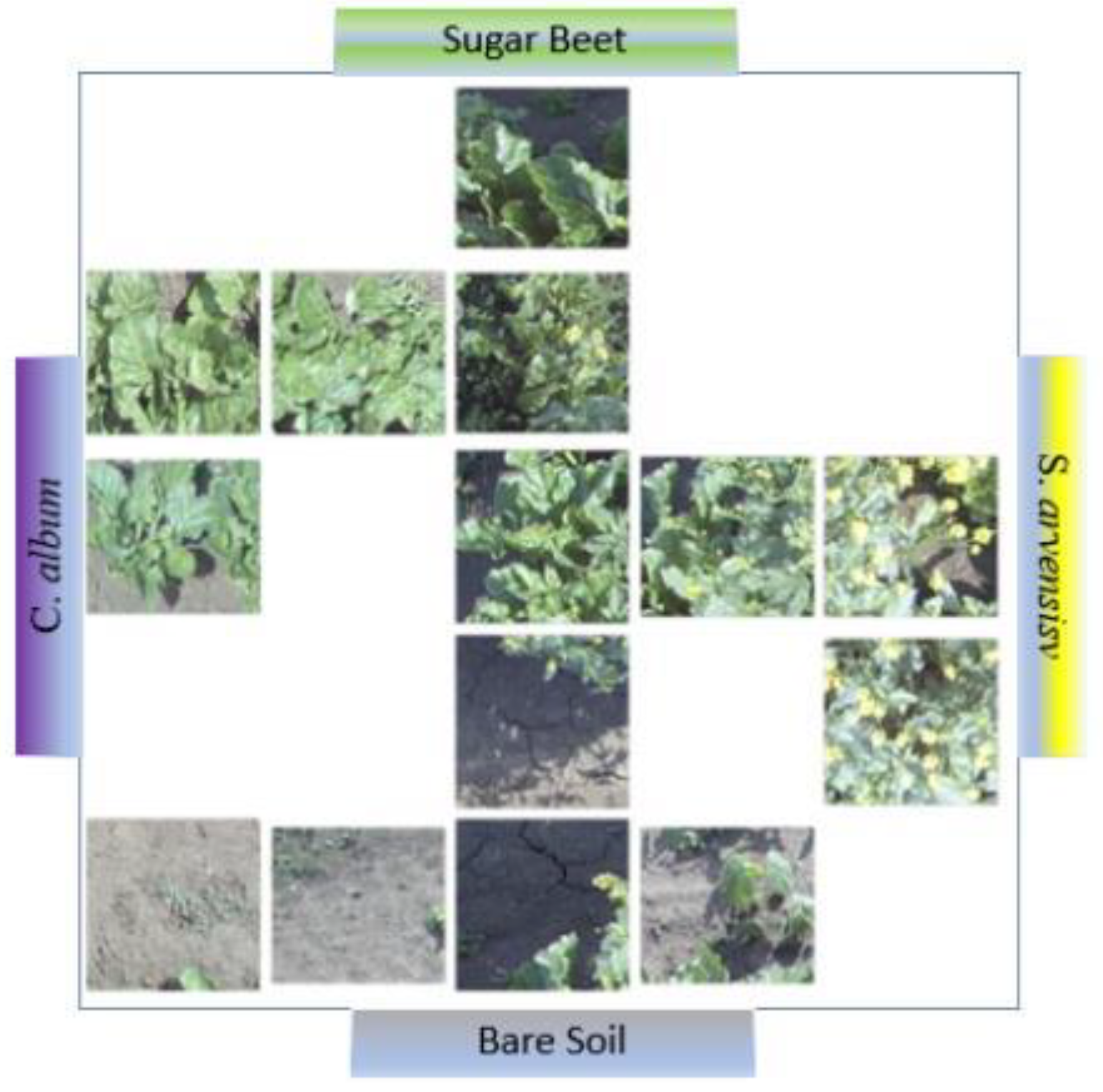
A quick overview of the ability to perform accuracy prediction is offered in
Figure 14, where the 14 test images are shown in a scheme according to their classification. A precise arrangement can be observed, including the relative gradual passages from one configuration to another.
3.4. Predictions
The aerial 4K photo of
Site B (
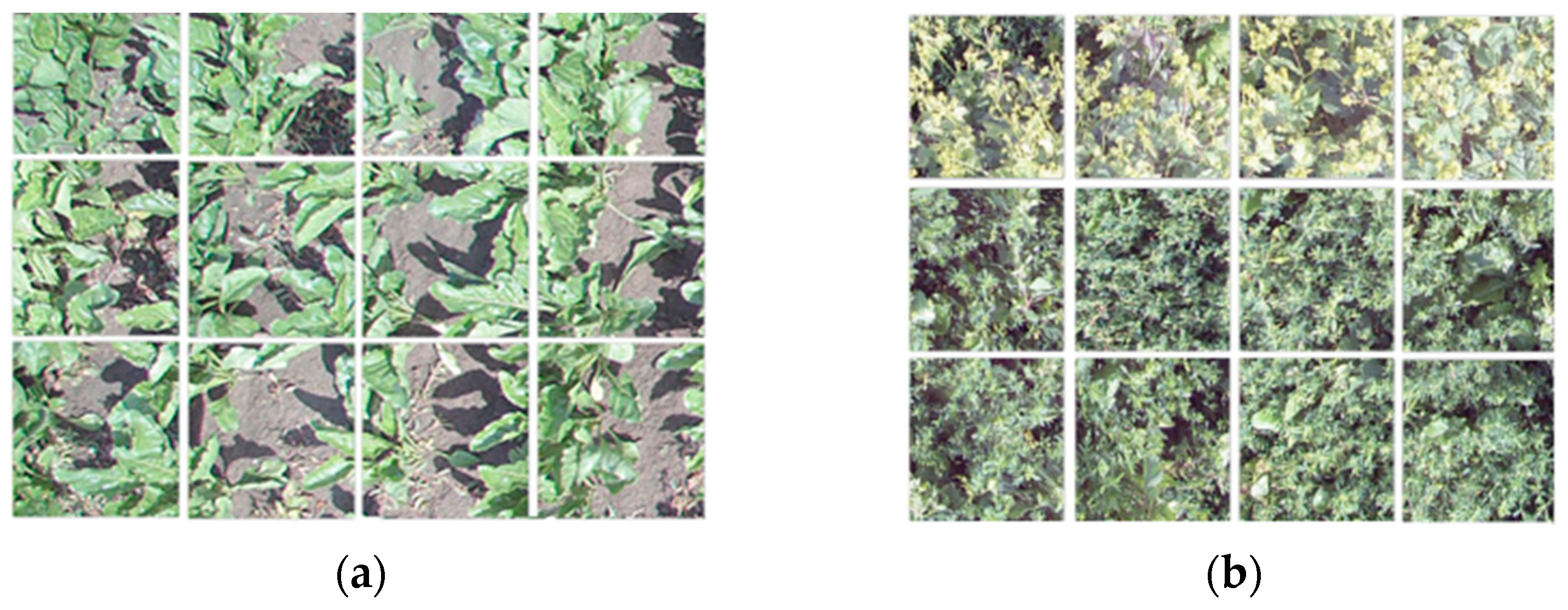
Figure 5b) was automatically framed using a 16 × 8 grid. An image dataset consisting of 128 tiles of 250 × 270 pixels each was then obtained. These pictures were embedded and clustered as previously discussed. Since no target cluster was preliminarily defined for such images, it was not possible to use this information to verify the hierarchical clustering efficacy as in the previous cases. However, browsing the different cluster of images, it seems a correct grouping was possible based on the (cosine) distance. This is evident in
Figure 15, where two different clusters are displayed as an example. In
Figure 15b, it is also evident how
S. arvensis and
C. album can be categorized in the same macrocluster when the vegetation is mixed.
The distance metrics can be conveniently applied to search for neighbors. In other words, it is possible to identify which images from the training dataset are closest to a determined image to provide an initial clustering. Even if it is not based on machine learning but on metrics, such a method can act very quickly and effectively, as shown in
Figure 16. It displays the three closest images in the training dataset (from
Site A) with respect to representative images from the testing dataset (from
Site B). In such a way, the category of training images can often be transferred to the testing images directly. This is the case, for instance, for the first image, which was found to be identical to three images from the training dataset classifiable as sugar-beet. Similarly, the second image from
Site B can be easily classified as
S. arvensis, since it is substantially indistinguishable from the three neighboring images from
Site A that were already categorized.
Even more interesting is the information offered by the metric distance about the other images. For instance, the third image clearly highlighted an intermediate situation that the classifier tried to clarify by recognizing three different classified images. In order of prevalence, it detected the presence of sugar beet leaves, which did not entirely cover the ground. It added the C. album visible in the upper left corner, ending with the third image to include a generic categorization of soil mixed with traces of plants. The classifier also proposed valuable feedback for the fourth photo. It correctly recognized the presence of C. album, partially in shadow, but it also highlighted the presence of S. arvensis in traces, which was less obvious.
Finally, predictions were also obtained with respect to each of the mentioned learners. Since all of them showed insignificant differences in accuracy during the cross-validation (apart from CT, which was discarded for this reason). Thus, at the moment, there is no particular reason to prefer a specific classifier with respect to the others. Therefore, all classifiers were taken into consideration for an initial analysis. Regarding the ability to identify the sugar beet, NN was the best: it recognized the presence of
B. vulgaris (with a probability over >50%) in the largest number of cases, 51 tiles out of 128. The other classifiers provided similar predictions but reported smaller groups: kNN, 34 images (with >40% probability); LR 27, (>51%); RF, 27 (>30%); SVM, 22. However, these image datasets were superimposed for the most part with NN and kNN methods to fully identify all the independent elements: 57 tiles out of 128, equivalent to 44.5% of the cultivation field. The results were manually checked to confirm the correct attribution. Some identifications are reported in
Figure 17, together with their prediction probability (by NN): a decrease in this probability corresponds to the beet leaves becoming sparser.
4. Discussion
The present work was aimed at identifying and validating a simplified methodology for species identification based on surveying cropped land with drones. The approach was proven to be effective in discriminating weeds from both bare soil and crop canopy. However, several considerations deserve to be introduced and discussed here.
4.1. Characteristic Dimensions
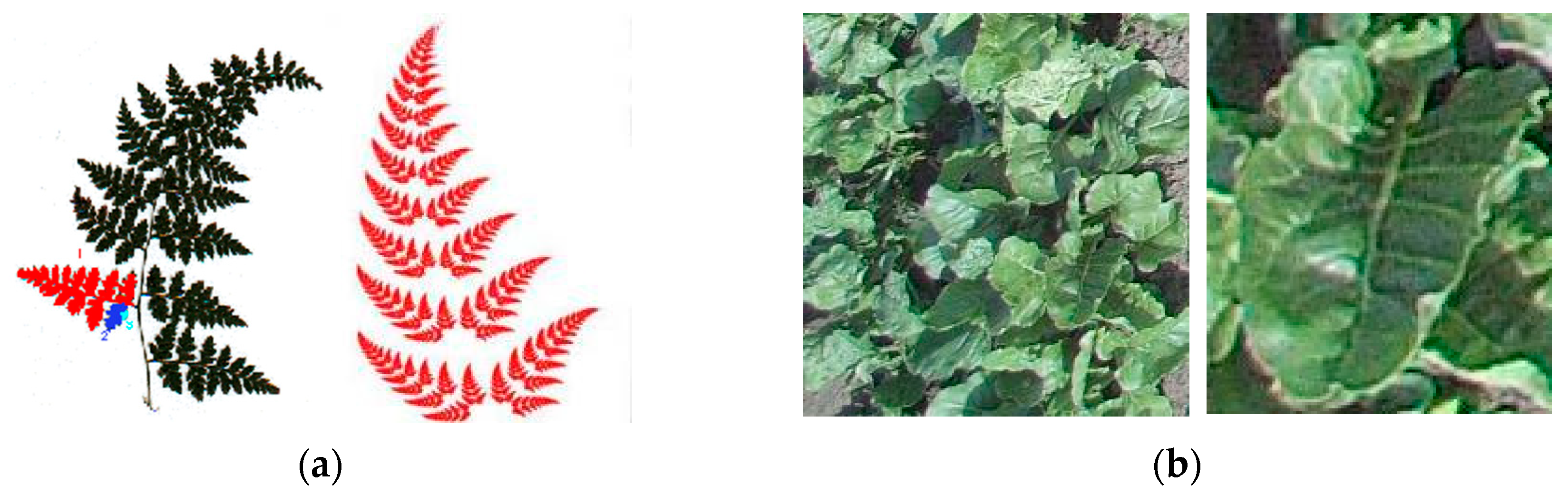
The height from which to carry out the photographic shots was considered in the analysis. Image analysis and pattern recognition often depend on characteristic dimensions and thus on the height images are taken at. This occurs when geometric structures are not homothetic: the property of repeating shapes in the same way on different scales (as happens for fractals). In the case of the foliage and leaves under investigation, enlarging or shrinking any part of them does not permit us to obtain new figures similar to the original ones.
The traditional example of homotheties offered by the leaf of a common fern, compared with the profiles of a sugar-beet in
Figure 18, makes the difference evident. Since part of the fern is similar to the fern, as a small copy of the whole, it can be reduced to smaller parts without losing its characteristic shape. This is not what normally happens with the images under consideration in the present research (
Figure 18b), making it necessary to analyze them on different dimensional scales.
The absence of an evident homotheticity in the problem also confirms the choice to carry out a study that was not based on fractals (as proposed, e.g., in [
36]).
Similarly, it was decided not to mix images taken at different heights: each dataset included images from a specific height. In this regard, although a systematic study was not implemented, some preliminary analyses were made with valuable conclusions:
- -
The height of images capture represents a crucial factor in the investigation but it is not fully independent: the camera resolution and width of field, as well as the process of image partitioning, are also involved.
- -
Several tools and metrics for image analysis can be used to relate graphic patterns regardless of their size. Moreover, modern image embedders consist of deep learning algorithms that are very robust with respect to problems of poor image quality.
Preliminary comparison suggested that the flight height of the drone with the camera was not as important for the image quality/resolution as the size of the portion of vegetation detected, as the type of vegetative patterns that machine learning has to recognize strongly depend on it (
Figure 19). In fact, when images taken from different heights were processed to arrange similarly sized sub-images, the end results did not significantly differ.
It was also indirectly demonstrated as follows. After the above investigation, further images were added with respect to three different criteria:
- (a)
Images taken from a different height (higher or lower);
- (b)
Images taken from the same height, merged, and scaled;
- (c)
Images taken from a catalog of aerial images of similar fields.
In no case did these new images improve the accuracy in the cross-validation.
The best results were achieved when the datasets consisted of images with sizes able to capture a single large beet leaf (such as 256 × 256 pixels from 5–7 m).
4.2. Hue-Based Method
The semiautomatic procedure for selecting the training pictures developed here is based on a hue-based process for picture partitioning that creates a collection of tiles, and each was assigned to a category based on the number of pixels with a hue value within the spectrum range assigned to each species. The pixel ratio (here called the discretized species coverage index—DSCI), combined with a user-defined threshold, can be considered a common color-based image segmentation method (as in [
37]).
The hue method was chosen, and an appearance parameter model was successfully developed to show only color information since the hue in the HSV/HSL/HSI color space should remain the same. Such an ability is very useful when, as in our case, illumination can vary in relation to the specific locations and conditions in which a photo is taken (e.g., different shooting angles or lighting angles). Evidence is provided in [
37], wherein changes in hue values, RGB, and grayscale were analyzed with respect to different conditions. The study includes objects characterized by primary colors of red, green, and blue, varying their shades (dark vs. light), location (indoor vs. outdoor), and illumination intensity (dark vs. bright). The experimental results show minimal variations in the hue values against drastic changes in RGB values, highlighting that objects’ color cannot be properly differentiated with weak light. In contrast, grayscale can differentiate objects well when based on brightness, as its value for brighter objects or illuminations was larger than that for darker objects or illuminations.
As a consequence, a combination of hue and grayscale was selected as the method in the present investigation, with valuable results. For instance,
Figure 20 shows how the identification of the albedo component on the spectrum (the yellowish component of the bare soil) can be performed by hue spectra analysis and used for the correct identification of shapes (i.e., the shadow).
Moreover,
Figure 21 shows how the effect of the intensity of different wavelengths of the solar spectrum affects hue values in terms of the mean (µ) and standard deviation (σ), masking weed texture. The density plots in the cases of
Site A and
Site B are reported, clearly showing two different peaks from more uniform image regions (σ~0), while a bell-shaped region centered around the central values of the hue covers the rest of the area. It is worthwhile to recall that hue values map in the range of 0:360 colors from red to blue.
A further analysis considering such values showed a high sensitivity of the response in the case of lower altitude images and smaller discretization windows (i.e., tiles). It was also evident that better results could be achieved when the smoothing process was performed with respect to the smallest windows (5 × 5 pixels), while better efficiency (R= I/S) was obtained for images from 25 m altitude processed by a 15 × 15 pixel window.
4.3. Applicability in Autonomous Systems
As noted above, this research had the main aim of developing a practical method for vegetation mapping (e.g., discriminating crops from weeds) as a way to guide autonomous systems in agricultural tasks (e.g., VRHS). For the scope application maps, as shown above, the results represent a first important step: data matrices are now available, wherein each cell provides an estimation regarding a specific geo-referenced (very small) portion of land inside a (large) agriculture field with respect to categorized elements (such as, e.g., B. vulgaris and S. arvensis in this case).
Different information can be provided by these maps depending on the use they are intended for. It is possible to simplistically report if it is necessary to provide a treatment (or not) in a certain area, as well as to indicate the probability/estimated content of each of the elements under consideration to design general intervention strategies.
Maps can be finally transferred to an autonomous system, e.g., by wireless protocols, to embed them in the navigation controller (this is part of ongoing research). Different logic layers may be involved. Depending on the level of integration permitted, application maps can be conveniently used by the system to aid in:
- (a)
performing tasks (e.g., spraying or not spraying in a specific area according to the presence or absence of a crop or weed);
- (b)
elaborating mission and strategies (e.g., optimization of routes).
Currently, the first case is quite popular and is performable by robotic systems equipped with smart spraying bars: while the autonomous tractor or robot is moving in the field, ‘smart’ spraying bars, wherein the sprayers can be independently activated, apply the chemical, optimizing application quantities. They are geo-locally controlled by the same system that controls the autonomous vehicle by logics implemented based on prescription maps as herein developed. Although many past and ongoing studies have addressed the development of
agrirobots that are as autonomous and efficient as possible, to the best of the authors’ knowledge, commercial robots able to accept such complex missions are not yet on the market [
38].
Figure 22 shows two alternative ways of representing the information that can be finally transmitted to the autonomous system to guide its action: (a) discrete levels to directly guide the intervention and (b) the continuous value probability to monitor the field.
This approach is not dissimilar to that discussed in a recent study [
39] wherein the opportunities of using UAV and recognition algorithms to monitor agricultural systems were explored and validated. Even if geo-localized data were processed by less effective methods for image analysis (i.e., maximum likelihood classification), they were similarly able to discriminate between weeds and surrounding elements with accuracy.
4.4. Specificity Achieved
For the above applications to be possible, specific measures with the aim of fostering image analysis and recognition were implemented to:
- (a)
consider the (very common) cases of overlapping of several vegetative species. This was done by converting the probabilistic estimates offered by the different classifiers into a measure of presence. For example, where the classifiers indicated a 60% probability of being ground and 40% of finding beet, the final indication was 40% beet in that area on a larger section of soil.
- (b)
manage the cases with comingling of several vegetative species (uncommon in real cases). This was done in the face of inconclusive probabilistic estimates of the many classifiers by adding a category that recognized such soil conditions.
- (c)
counteract the masking effect due to the presence of shadows. This was achieved using a hue-based color model that is recognized to be superior to others.
- (d)
counteract the distorting effect of the image capture height. This was achieved by combining different techniques. First, images from different heights were integrated. Next, when the images were segmented, the segmentation was rearranged several times, modifying the procedure to obtain different sets of sub images. This approach also allowed for a large increase in the dataset for machine learning training. Finally, in the detection of similarities between images, metrics that were not sensitive to the zoom of the shapes were chosen.
- (e)
reduce the image complexity, avoiding a slowdown in the recognition procedure and the risk of overfitting. This was achieved by applying PCA to data to identify and isolate the main components. It reduced the characteristics needed to distinguish one image from another from a few thousand to a few hundred with a quite similar accuracy.
5. Conclusions
Precision agriculture is a rapidly emerging area of investigation due to the enormous advantages it offers in terms of production efficiency and environmental sustainability. For instance, knowing with extreme precision the amount of water, fertilizer, or herbicide to release at each point of the cultivated field is a key element for the agriculture of tomorrow. A great deal of trust has been placed on precision agriculture by humankind with respect to its capability to increase food production, improve quality and safety, and decrease negative anthropogenic impacts. Various precision agriculture interventions have shown how these hopes could be well placed over the years. Agricultural techniques for working the terrain with precision, in geo-localized form, are maturing.
Many new, fascinating, and innovative ideas are also emerging. For example, the authors of this study are involved in a project to implement an autonomous robot for weeding by laser technology. Similar agricultural rovers and robots can be effective only when precisely guided in their actions. The problem this article was intended to address is apparent, i.e., how to recognize what to do, and we wanted to offer a practical answer.
An open source and easily usable machine learning tool was proven to be able to distinguish with extreme precision the areas where the crop (i.e., B. vulgaris), weeds (i.e., C. album and S. arvensis), a mix of both, or bare soil are present. The tool therefore enables guidance of a ‘geo-localized automatic tractor’ by determining how to intervene in each area. Within this scope, an answer to another problem, often ignored, was proposed: how to provide convenient information to the artificial intelligence system so that it can be properly trained. Specifically, it was shown how a single aerial image, taken by a small commercial drone and a common digital camera, can be used for this purpose. The image was fragmented into differentiated panels by applying basic concepts of image analysis and color filtering. These concepts would not have been able to accurately distinguish the areas to be treated when applied alone; however, the combination of these techniques makes it possible to quickly separate the images into categories, discarding data that is vague or superimposed. These selected images were used to train an intelligent system that was able to recognize what was present in areas it had never observed before. One of the secrets of this success is the consideration, among the many image analysis engines, of a method designed to recognize the paintings of artists. The images are broken down into colors, shapes, and styles according to more than two thousand different parameters of comparison to generate that knowledge, which then allows us to understand exactly how to intervene. At the same time, it must be considered that the study was focused on a two-weed dominant-species scenario that permitted the validation of the method in a controlled environment (experimental plot). Future analysis will include additional complexity, both in terms of different species and observations throughout the cropping season.


