1. Introduction
In the last years, different urban railway platforms have been reaching high levels of density, affecting the experience of traveling and therefore the quality of life [
1]. For example, in the case of Chile, the Metro de Santiago reached more than 2.5 million trips per day (i.e., about 700 million passengers per year), in which the platform–train interface (PTI) is perceived as the space where more interactions occur [
2,
3,
4,
5,
6]. Likewise, in the case of other train systems in the world such as the UK railway network, each year there are more than 3 billion interactions, and half of the fatality risks for passengers occur on platforms, being complex spaces that present different risks and dangers for passengers [
7,
8].
In situations with high passenger flows, e.g., densities greater than 5 passengers per square meter at the PTI, the efficiency and safety of the entire system are affected [
9]. Regarding efficiency, for high-frequency services, the dwell time of a train in the station is the main component of station capacity, which is related to passenger behavior [
10,
11]. From a safety point of view, an increase in passenger density can cause accidents at the PTI. For passengers with reduced mobility, such as wheelchair users, the PTI is a complex space due to safety reasons, for which a strategy is needed to reduce accidents and improve the travel experience [
12,
13,
14]. Passengers can be trapped, fall onto the tracks, or stumble aboard trains, sustaining injuries [
15,
16].
To improve efficiency and safety at the PTI, public transport operators can activate crowd management measures (e.g., the platform is closed), and passengers are contained in an earlier stage (e.g., at turnstiles, ticket offices, or outside the station at street level) [
2,
3,
4]. Moreover, due to COVID-19, crowd management measures have been implemented [
17,
18]. In the case of the Metro de Santiago, Fruin’s Level of Service (LOS) is used [
10,
11,
19] to classify the level of congestion at the PTI, in which different types of passengers are needed to be included [
20]. The congestion at the PTI depends mainly on the time getting on and off, the number of passengers getting on and off, and the time of opening and closing the doors [
10,
11]. According to Aashtiani and Irvani [
21], the congestion at the PTI is affected by the number of doors, the vehicle load factor, and the method of charging fees. Similarly, Harris [
22], based on the London Underground, identified that the congestion at the PTI depends on the time required to open and close doors, the number of doors per vehicle, the door width, the number of passengers boarding, the number of passengers getting off, and the number of seats per vehicle, among other factors.
In addition, the congestion at the PTI is influenced by passenger density and vehicle and platform layout. According to Harris [
22], if there are few passengers, passengers have enough space to get on and off simultaneously. However, when there is a crowded situation, passengers will wait until the alighting is complete or until there is a space available to board the vehicle. Other studies presented by Wiggenraad [
23] suggest that wider doors decreased the congestion at the PTI. However, the relationship between door capacity and door width appears to be nonlinear. This is also supported by Heinz [
24] who studied the difference in height between the train and the platform and found that the congestion increased when the number of steps increased. No problems were observed when the horizontal distance between the train and the platform was less than 5 cm; however, problems were observed for the passengers when this distance reached a value greater than 15 cm.
More recent studies [
25] indicate that congestion at the PTI is a function of the fare collection system, the type of passengers, and the amount of crowding situation, among other factors. Surveys have been conducted by Currie et al. [
26], in which the congestion was found to be influenced by the number of passengers on board (congestion inside the vehicle). Christoforou et al. [
27] studied this congestion using data collected from an automatic passenger counting system on board urban light rail systems. The authors state that the volumes of boarding passengers, alighting passengers, and passengers on board affect the LOS, as well as vehicle design (e.g., low floor), time of day, and station location. Li et al. [
28] proposed a model for Dutch railway stations when the demand for passengers getting on and off is not available on real-time. In the case of metro services, D’Acierno et al. [
29] reported a new methodology based on crowding on platforms and the behavior of passengers getting on and off. Furthermore, Yazdani et al. [
30] established that the allocation of seats could affect the congestion in rail systems. Moreover, in the case of delays and queues in stations caused by the excessive time taken by vehicles completing their electric charge or visual inspection, Ullah et al. [
31] proposed to include precise planning in which knowing the availability at the station to reduce congestion is required.
Although there are important advances in the literature, these models and field observation approaches are based on existing stations, which limits the analysis only to the trains and platforms that currently exist, without being able to know the density of passengers at the PTI in real-time and, therefore, only through observation can the congestion be estimated, as for when it might be necessary to activate a crowd management measure. This visual inspection method makes it impossible to generate measurements in a standardized and automated way, depending on each inspection and the interpretation of what is observed. Furthermore, the effect of these measures on the density (i.e., the inverse of the personal space) is unknown, and therefore their impact on passenger behavior is not quantified for different types of passengers. For example, when wheelchair users are boarding the train, there is an additional time required for the opening and closing of doors, the time to unfold and retract ramps, and the additional time it takes for each wheelchair user to reach a reserved area inside the vehicle, which is not necessarily included in current models.
To address the above problem, a new method is developed to estimate the density of passengers waiting to board urban railway platforms by means of laboratory experiments, which is the main objective of this study. The specific objectives are: (a) define the experimental set-up to represent a carriage of a train and its adjacent platform; (b) define the parameters to detect passengers boarding and alighting; (c) develop a method to estimate the density of passengers using Voronoi polygons; (d) evaluate the errors and the density obtained using the method compared to the LOS.
The structure of the paper is divided into five sections. In
Section 2, different studies of passenger interaction in the process of boarding and alighting urban railway systems are reported. Next, in
Section 3, the experimental method is described. In
Section 4, the results are analyzed, followed by the conclusions in
Section 5.
2. Passengers’ Interaction in the Boarding and Alighting Process
To address the problem presented by models and field observations, different studies based on full-scale experiments have allowed the testing of different station configurations to reduce congestion and improve efficiency and safety at the PTI. Regarding the interface design, Fernández et al. [
32], in the Pedestrian Accessibility Movement Environment Laboratory (PAMELA) of the University of London, reported that congestion depends not only on the number of passengers getting on and off but also on the platform height, the width of the door, the method of fees collection, internal vehicle design, and vehicle occupancy. Another experiment conducted by Rudloff et al. [
33] showed that the congestion decreased as the width of the door increased.
According to Holloway et al. [
34], the use of steps has also been shown to affect the congestion at the PTI, in which the passengers getting on took longer (4.13 s on average) than those who get off (3.68 s on average). Recently, some authors [
2,
35] reported in PAMELA that the use of platform edge doors does have an important impact on the congestion of passengers, influenced by other variables such as the formation of flow lines, distribution of passengers, the distance between passengers, and the speed and space used by each passenger. To reduce the congestion, Seriani and Fernandez [
3] reported that a rectangular area should be used in front of train doors as a “keep-out zone” to prevent passenger boarding from being an obstacle for those who are alighting. These authors concluded that the experimentation allowed the testing of different designs for the vehicle–platform interface based on existing stations, where a single variable changes while the rest of the variables (for example, light, sound, information, physical design, etc.) remains the same. In this way, laboratory experimentation makes it possible to control the variables and to use computer vision tools for pedestrian study.
To measure the interaction at the PTI, Shen [
36] proposed two main areas: circulation and waiting zones. Both areas have their own characteristics and functionality for passengers. Passengers in the waiting areas behave differently from those who are in the circulation zone. For Wu and Ma [
37], there are two main types of interaction between passengers who are waiting: queuing or clustering to the side or in front of the train doors. One of the main variables, which is common in both types of interaction, is personal space. As reported in the HCM [
10,
11], in any standing area (e.g., PTI), a pedestrian can be represented as an ellipse of area 0.30 m
2 comprising a body depth of 50 cm and a shoulder breadth of 60 cm [
19]. However, when the pedestrian starts to walk, this area increases to 0.75 m
2 because there is extra space used for leg and arm movements [
38]. In the presence of obstacles, Gérin-Lajoie et al. [
39] reported that pedestrians need a space represented by an ellipse of area 0.96 m wide by 2.11 m deep, which is smaller when overtaking a static versus a moving obstacle. In addition, Gérin-Lajoie et al. [
40] demonstrated that this space can be asymmetrical in shape and side (left and right) during the circumvention of a cylinder (or column) as an obstacle, in which the longitudinal axis of the ellipse is related to the speed. These studies are related to the concept of the sensory zone, which is “the distance a person tries to maintain between the body and other parts of the environment, so there will always be enough time to perceive, evaluate, and react to approaching hazards” [
41]. For example, for a normal walking speed, the sensor zone can be estimated as an elliptical area of 1.06 m wide by 1.52 m deep. Similarly, Fruin [
19] calculated that the sensory zone reached a distance of 1.48 m for a normal walking speed of 1.37 m/s.
Other studies [
42] reported that older people need more space to move in high-density situations. However, this increase can be moderated with social support and self-control. In this sense, Webb and Weber [
43] state that personal space is affected by vision, hearing, mobility, age, and gender (e.g., when mobility is reduced, each pedestrian needs more space). In addition, Sakuma et al. [
44] reported that personal space is defined by an inner critical circle, within which there is immediate avoidance of any agent appearing in it, and by an external circle where caution is applied to avoid pedestrians who appear there. According to Daamen and Hoogendoorn [
45], other characteristics of pedestrians should be considered, such as age, gender, and health. In addition, the authors identified that walking purpose, route familiarity, and luggage can affect the interaction of pedestrians. Similarly, Willis et al. [
46] state that men walk faster than women. The authors also found that age, mobility conditions (e.g., bags and luggage), and time of the day affect the walking behavior of pedestrians. Other studies [
47] also include the effect of cultural differences, for example, the speed of Indian pedestrians is less affected by density, whereas it does affect the speed of German pedestrians. The effect of intimacy is also affected by culture, which was first studied by Hall [
48], in which the intimate distance was classified into different groups according to the relationship between pedestrians. For example, if the distance between two pedestrians’ heads is less than 1 m (taking into account 0.5 m plus two times half the body depth reported by Fruin [
19]), then pedestrians will feel that their space is being invaded. However, this feeling of invasion is based on perception (e.g., comfort) rather than physical space (e.g., available space or density), which is difficult to calibrate at the PTI zone [
49].
To measure this interaction, it is necessary to use technological instruments. In the case of observation at existing stations, the use of videos and passenger counting tools enables the interaction of passengers at the PTI to be identified [
4]. However, currently, the extraction of videos for subsequent analysis presents challenges, with automatic detection through computer vision being one of the most relevant [
50,
51,
52,
53]. Although there have been improvements using computer vision at the PTI, this space in metro stations presents some problems to solve which involve occlusion, recognition of people in a high-density crowd or using mobility aids, and interactions between people waiting to board the train, among others [
54]. Consequently, manually counting people using videos takes a long time in terms of data capture and analysis, and therefore automatic counting systems are required to obtain the density at the PTI, which can be used to suggest a crowd management measure. Therefore, two approaches can be used [
55]. The first approach is to train a machine learning model based on swipe card data to infer the number of people on the platform, while the second one is to use cell phone signaling data to estimate the number of people on the platform. Both approaches are interesting and can be used as further research to compare the method proposed in this study with existing station data analysis.
3. Experimental Method of Detection and Estimation of Density
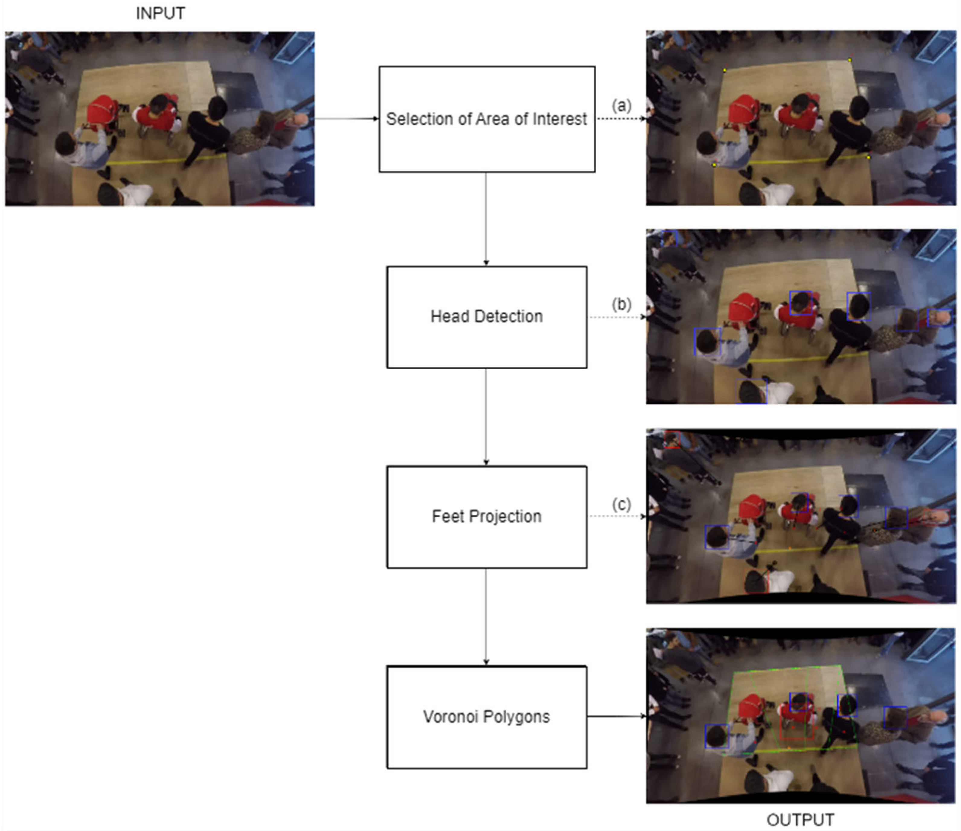
An experimental method is proposed to define the available area for each passenger boarding and alighting. This method is carried out through four sequential stages (see
Figure 1): (1) selection of the area of interest; (2) head detection; (3) feet projection; and (4) calculation of the available area per passenger using Voronoi polygons. Different from previous studies, the available area is calculated on the platform, and therefore occlusion problems are reduced, considering the feet projection of each passenger after detecting their heads. The reason for using the Voronoi polygons is that it helps to identify the geometric proximities of the projections of the passengers’ feet within the area of interest, allowing the identification of the available area for each passenger. In the following sections, the stages are explained to better understand the proposed experimental method.
Figure 1 shows dotted lines representing the virtual output stages, while thick lines are part of the flowchart. The virtual output in
Figure 1a shows the selected yellow points for the area of interest. The virtual output in
Figure 1b shows the heads detected (shown in blue squares) by the object detector. In
Figure 1c the feet-projection section calculates the projections and decides if each detection is inside the area of interest. In this stage, the red squares are detections discarded, while the blue ones are allowed. Finally, as an output, the Voronoi polygons (shown in green) are obtained, in which detected heads inside the area of interest (blue squares), the projections as red dots, and the orange dot as the reference point, are represented.
3.1. Area of Interest
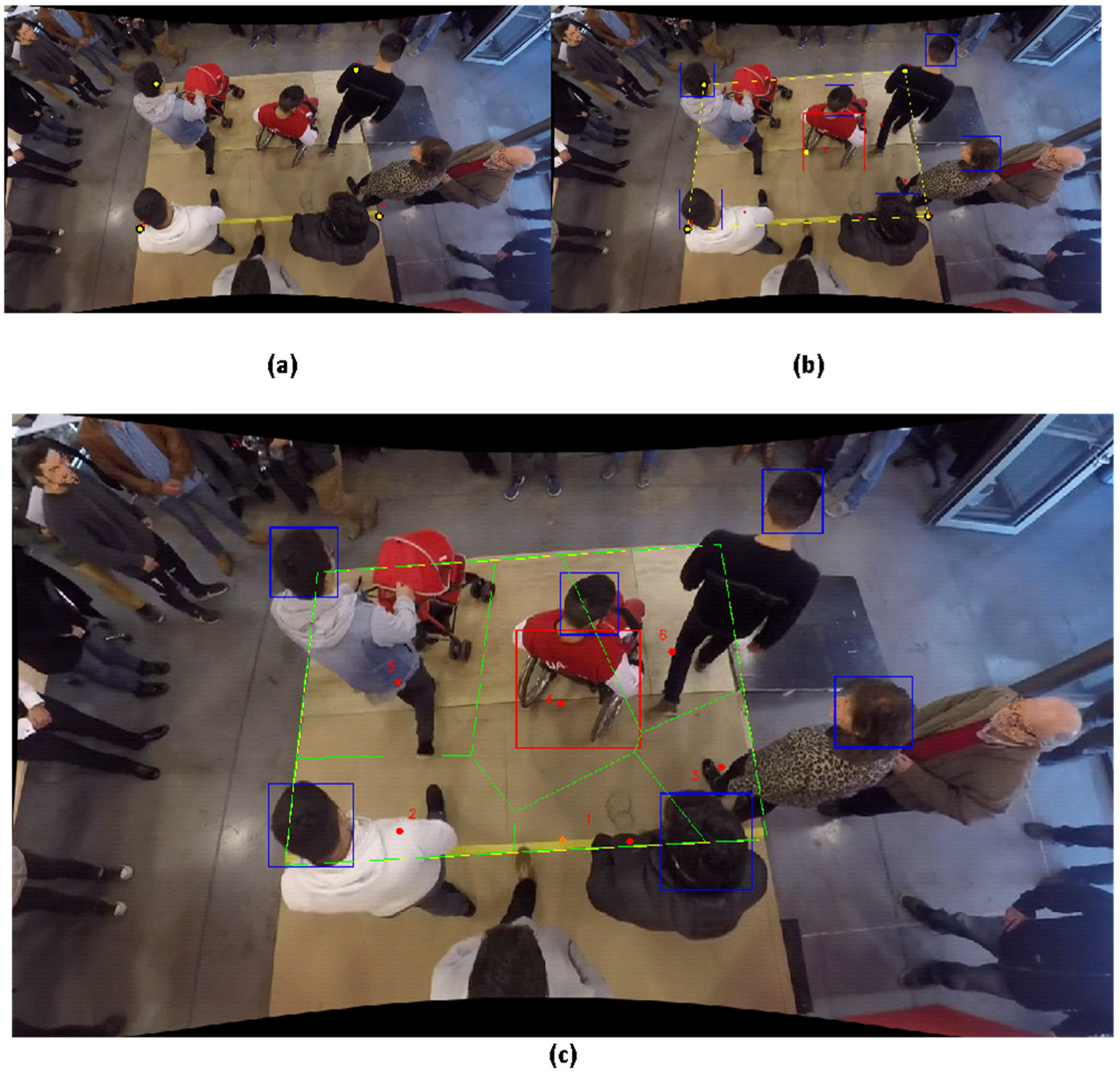
The area of interest is a polygon, i.e., a fully closed boundary, that satisfies the convexity property. This polygon, manually drawn on the image to be analyzed as a set of points, represents the zone to be measured, and its layout and area in square meters are assumed to be known beforehand. Because of the convexity property, the minimum number of points of this polygon must be three. The main purpose of this area is to encapsulate the zone which will be used for the Voronoi polygons and the corresponding occupancy surface per passenger.
Figure 2a represents an example.
3.2. Detection of Passengers
To detect each passenger and estimate the density at the PTI, a novel method has been used. This stage is related to the detection of heads through a Faster RCNN detector, which is a deep learning model trained specifically for this experiment. The second stage consists of explaining the estimation of the feet projection, continuing with the Voronoi polygons, which represent the area of interest for measuring the density of pedestrians. This selected area included the 6 m
2 on the platform defined in
Section 3.1.
For detecting heads, the selected object detection model was the Faster RCNN [
56] and InceptionV2 [
57] as its CNN backbone. Faster RCNN is similar to YOLO [
58], which is a model that works mainly with two modules in parallel. The first module is a deep fully convolutional network that proposes regions, namely a region proposal network (RPN), and the second module is the Fast RCNN detector [
58]. The RPN module indicates to the Fast RCNN module the places to consider. To generate region proposals, a small network must be slipped over the output feature map from the last shared convolutional layer of the CNN backbone. This small network simultaneously predicts multiple region proposals delivering data in parallel to the regression and classification layers. The regression layer encodes the proposal coordinates, and the classification layer estimates the probability of each proposal being an object or not an object. The InceptionV2 architecture extracts information from low to high-level features. However, this is not performed following the classical structure of a densely connected architecture (also known as fully connected), but by a sparsely connected architecture, where convolutional factorization and asymmetric convolution can be found. This network is 42 layers deep and uses batch normalization for training stabilization [
59].
This model was trained with images extracted from this experiment in a random way for head and wheelchair classes.
3.3. Feet Projection
This stage is used to estimate the coordinates of the feet of each detected person. This operation is achieved by scene projection, that is, from the real-world 3D scene to the projected 2D image.
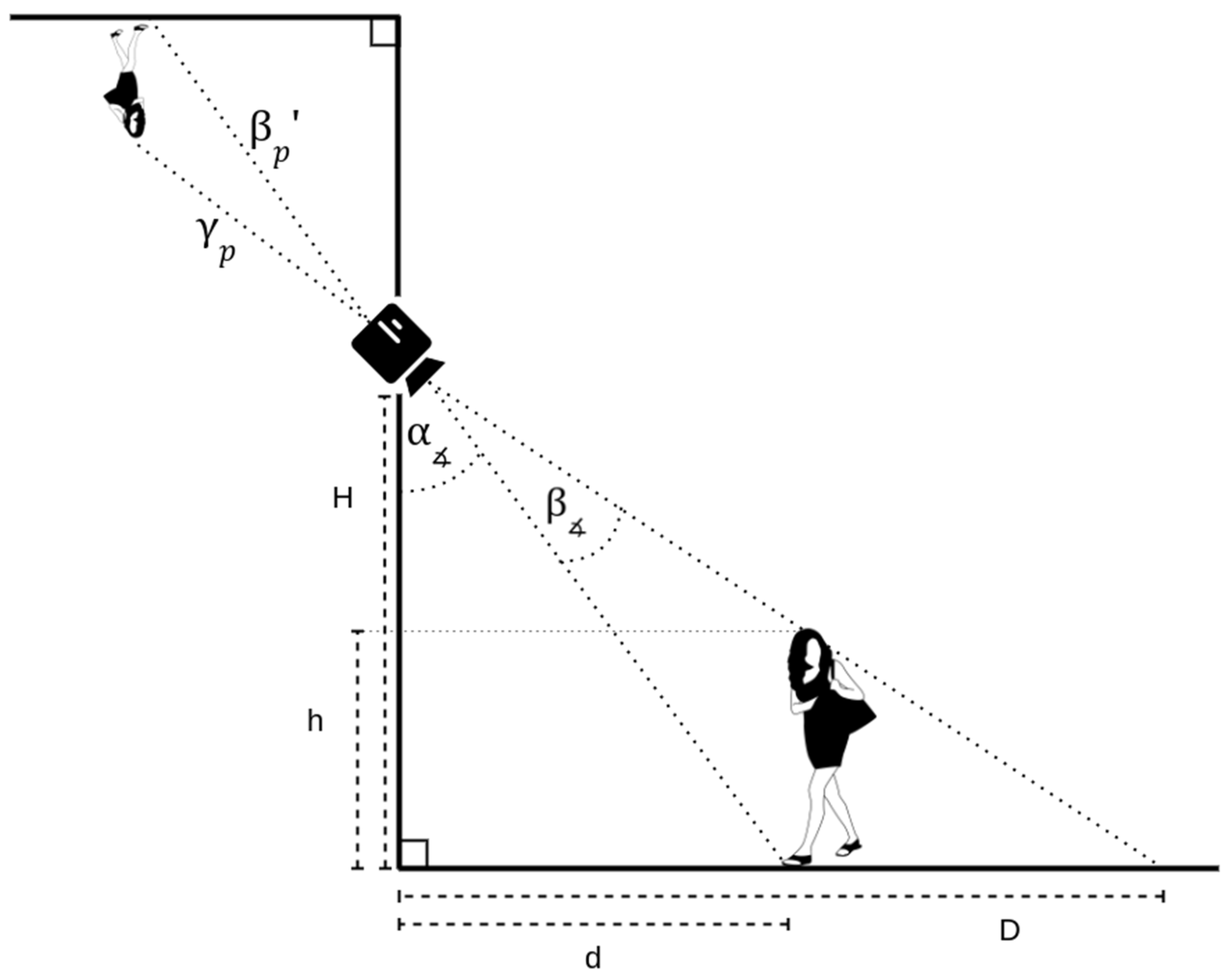
The camera used was a GoPro 5, which has a 90° FOV (Field of View). The height at which the camera was positioned will be referred to as H meters above the ground, and the angle normal (horizontal angle) to the floor is
φ. For the calculation of projections, it is assumed that all people in the images have the same nominal height h. The area of interest is a polygon, i.e., a fully closed boundary, that satisfies the convexity property. This polygon, manually drawn on the image to be analyzed as a set of points, represents the zone to be measured, and its layout and area in square meters are assumed to be known beforehand. Because of the convexity property, the minimum number of points of this polygon must be three. The main purpose of this area is to encapsulate the zone which will be used for the Voronoi polygons and the corresponding occupancy surface per passenger.
Figure 2a represents an example.
Thanks to the area of interest, a foot projection algorithm is used to alleviate the occlusion problem at the PTI, where crowded situations are likely to occur [
60,
61]. This stage also requires the object detection model. This requires setting a reference point in the image (shown in orange in
Figure 2c), which is obtained as follows:
where
is the reference point coordinate,
is the centroid of the convex polygon, and
is the height
H of the image, in pixels. As can be seen, the reference point depends on the angle of inclination of the camera and the positioning of the centroid of the polygon.
The centroid of each head is then expressed with
as the origin by:
where
represents the centroid vector of the head’s bounding box. Clearly,
is a pixel distance value. However, for a reliable estimate of the projection of the feet, the need to use information from the 3D plane arises, as shown in
Figure 3, from which the following equations apply:
where
corresponds to:
In this case, is equivalent to the L2 norm in the image, that is, , where is a tuple indicating both the height and the width of the image, respectively. In Equation (8), the weighting of π/2 occurs because of the FOV of the camera.
Once the value of is obtained, it is important to return its value in pixel units using the same process as Equation (8) but solving for for this case.
Although the objective of finding
was achieved, it should be noted that the captured scenes always depend on the camera angle of inclination, and therefore, the estimated values will be influenced by that angle. With this, we have the following:
In this way, we modify the value of by weighting it with the angle of inclination.
Finally, the coordinates of the feet
, for their respective person represented by
, are calculated as follows (Equations (11)–(14)):
After the calculations,
is obtained as:
where
is the slope between
and
.
Figure 2b shows an example of these feet projections.
3.4. Voronoi Polygons
Once the projections are obtained in a given image, a Voronoi polygon [
62] is calculated to estimate spatial occupation (i.e., the available area by each passenger or, equivalently, the inverse of density).
Given a metric space
,
is defined as a set of particles (e.g., passenger),
as the Euclidean distance
with
. The Voronoi polygon concept is established for each particle as the intersection of all half-planes.
where
is defined as
half-space:
Equation (16) denotes the half-plane of all points that are closer to
than to
. These cells can have different areas, as well as different numbers of borders. These cells are influenced by the neighborhood of
, so that two particles are neighbors if they share an edge. Every point on these edges is equidistant from both particles. Finally, these cells are characterized by being convex polygons.
Figure 2c shows the Voronoi polygons applied to the projections of the detections.
4. Results
4.1. Experimental Set-Up
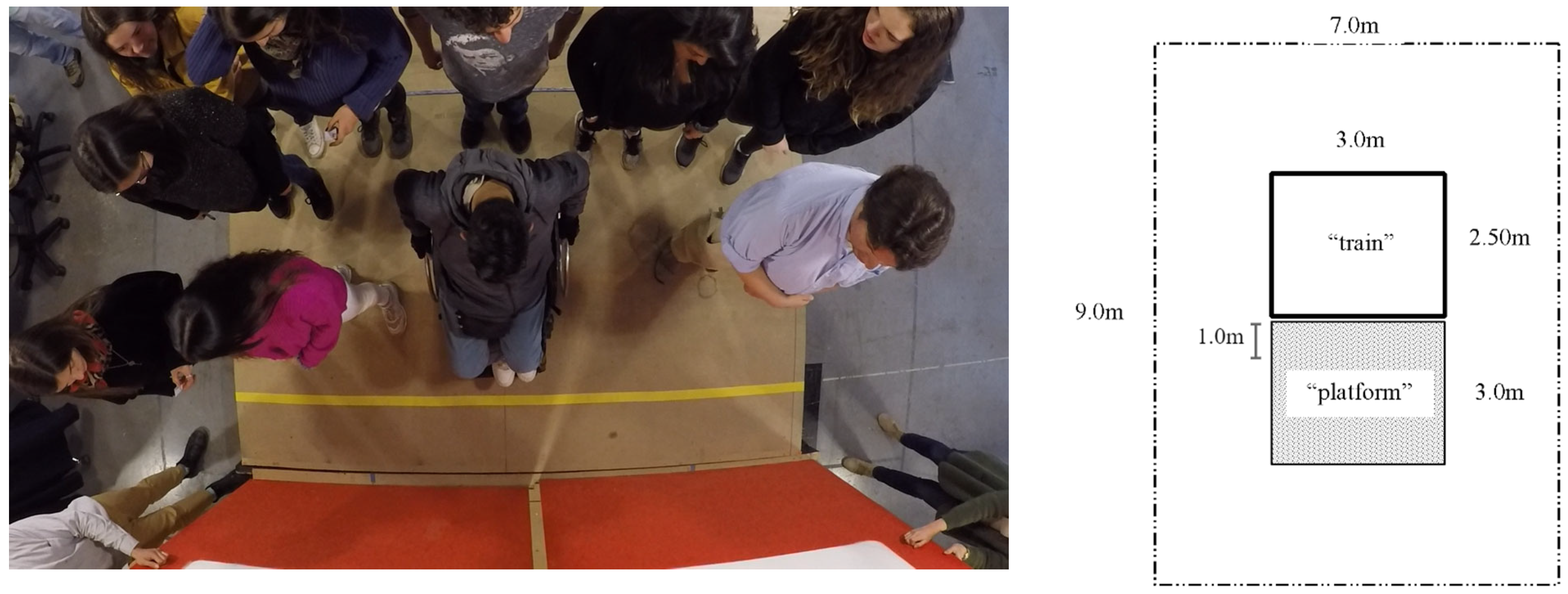
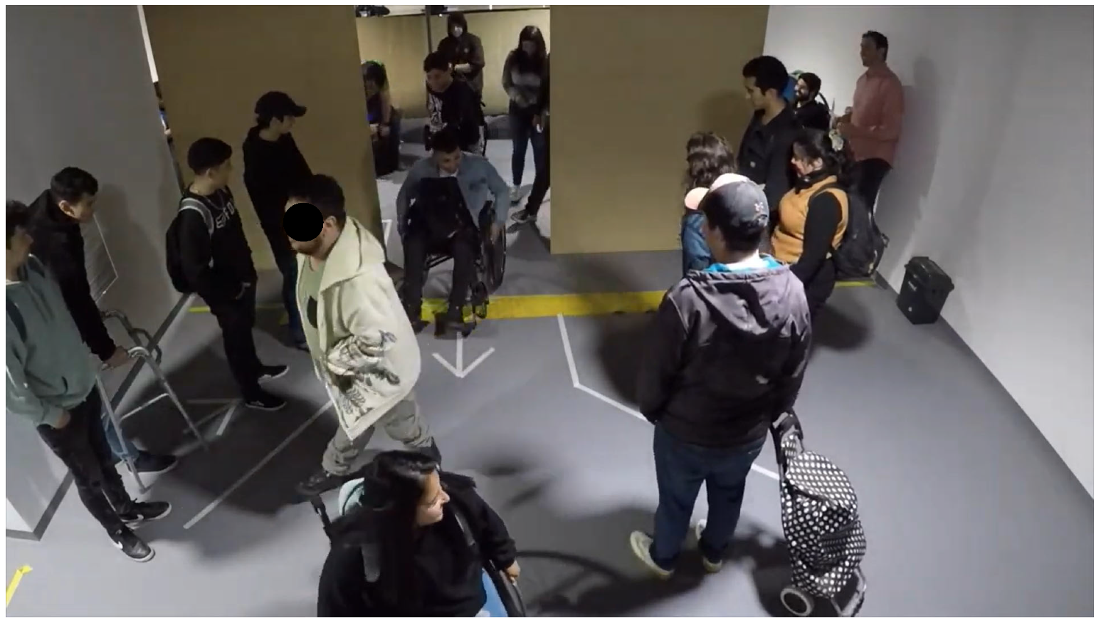
In order to carry out the experiments in a controlled environment (see
Figure 4), a mock-up was used to represent the PTI, in which the number of participants and the sequences of boarding and alighting were defined. In all the experiments, the platform had a length of 3 m to represent the boarding and alighting in front of one door. In addition, the platform had a width of 3 m, in which a yellow safety line was located 1 m from the edge of the platform (i.e., 2 m of effective platform width). In other words, the platform had an area of 6 m
2 (3 m long by 2 m wide), which is defined as the area of interest.
The experiments included a total number of 22 volunteer passengers, and therefore a density of around 4 passengers/m2. One passenger used a wheelchair and has used this mobility aid for 24 years due to spastic diplegia. The wheelchair user was a young person (between 18–24 years old) whose weight was 70 kg. Another passenger had a baby pram, representing a passenger with reduced mobility. Another three passengers also represented those passengers with reduced mobility as they were more than 60 years old and had difficulties walking. The rest of the participants (18 passengers) were young students (18–24 years old), who regularly used the metro system in Santiago de Chile.
Ten repetitions were carried out, in which users entered the train from the platform area to later get off the train once the doors were open. In this way, each of these repetitions of boarding and alighting consisted of three phases. In the first phase, participants entered the platform area randomly, thereby waiting for the arrival of a train. Furthermore, at this stage, five users were randomly told that they were in a hurry to get on the train, better representing a situation in existing urban railway stations. Then, in the second phase, the doors were opened, and all participants entered the train, ending with the closing of the doors. Finally, in the third phase, the doors were opened so that the users alighted from the train, and the phase ended with the closing of the doors.
4.2. Passenger Detection and Error Calculations
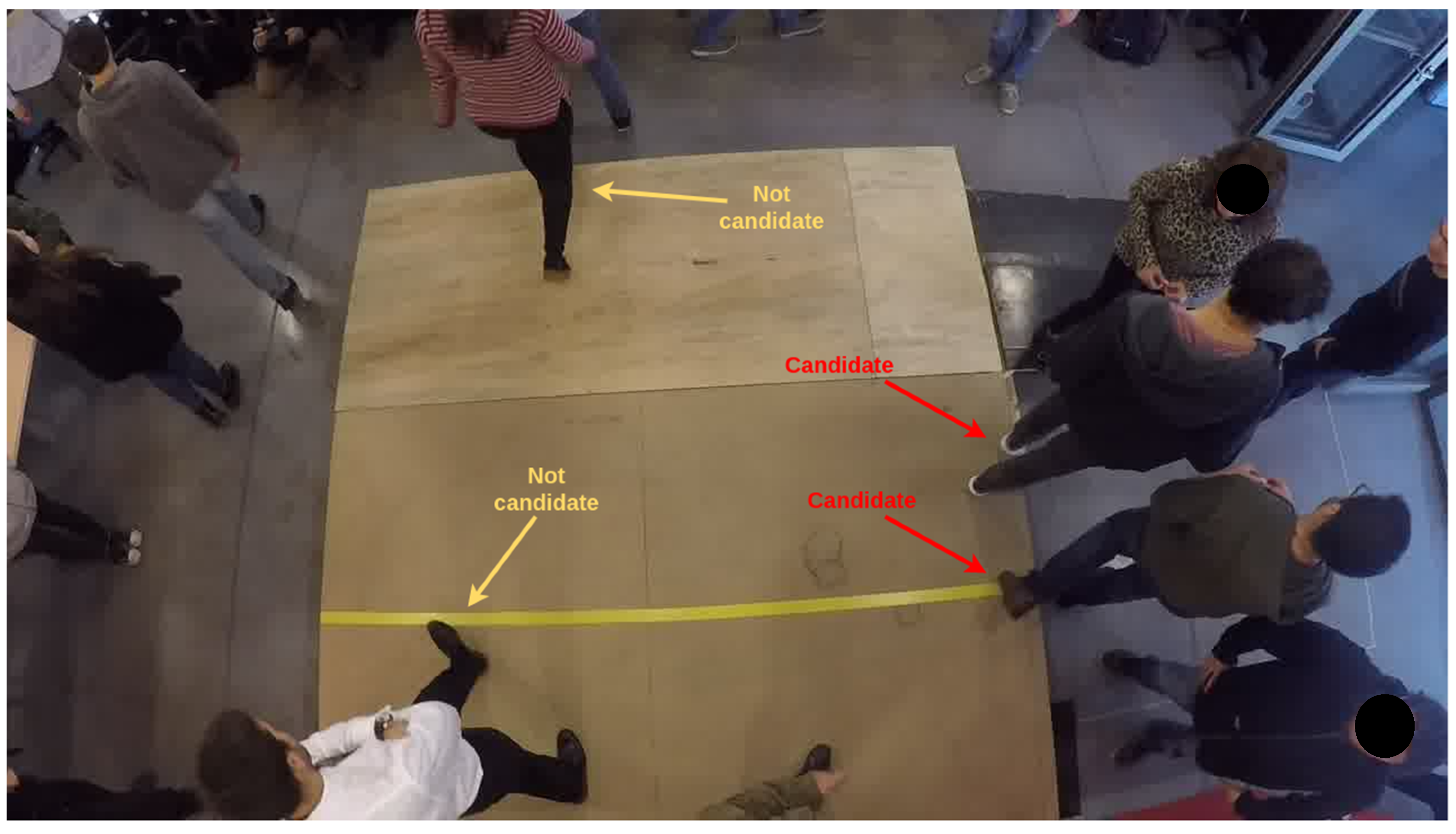
The experiments carried out were labeled based on the premise of how many people were, on average, inside the platform, that is, the target convex polygon. This task was carried out through rigorous labeling of each situation with the average area available per person (i.e., the inverse of the density). There were situations in which it was difficult to discriminate if the people were actually inside the polygon or not. A person was considered as a candidate within the polygon if they had at least one foot inside it, and if their head was visibly detected (
Figure 5 serves as an example).
The experiments were evaluated using the standard MSE (Mean Square Error) formula:
where
corresponds to the ground truth average area per person within the convex polygon in image
, while
is the average area per person within the convex polygon estimated by the developed algorithm, and
is the number of images.
Experiments were carried out using different parameters, such as the height of the camera (), the average height of the people (), and the number of people inside the convex polygon, using MSE to measure the errors in each case to assess the variability of the algorithm.
The error calculations of the algorithm were carried out. The image set used had 344 images, from 1 to 18 people. Additionally, the parameters of the experiments were with values of from 2.5 to 2.9 m with steps of 0.2 m; from 1.6 to 1.8 m with steps of 0.05 m; and with situations ranging from 1 to 18 people within the convex polygon. As far as verified values for the experiment were concerned, the values of = 2.7 m and 𝜑 = 14° were assigned.
Table 1 shows the MSE values for all combinations of
H and
h, and ground truths from 1 to 9 passengers within the convex polygon.
Table 2 follows the same process, but from 10 to 18 passengers.
Table 1 and
Table 2 show that there is variability in the algorithm with respect to the assigned parameters. However, apart from measuring the sensitivity of the algorithm,
Table 3 shows the values for the average error per experiment.
According to
Table 3, the best error averages correspond to
H = 2.5 m and
h = 1.6 m, and
H = 2.7 m and
h = 1.75 m. Another result, seen in
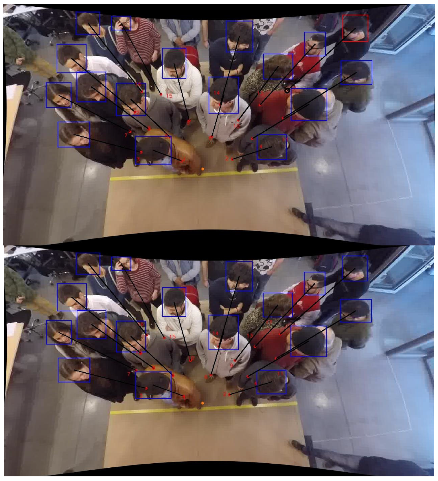
Table 3, is that those passengers who exceeded the value of h were not detected by the algorithm within the area of interest. For example, in
Figure 6, the same situations are presented for different values of
h. The difference between them is that the lower image reached an additional detection compared to the upper image. The red bounding box (upper image in
Figure 6) means that it is detection not considered in the algorithm since its estimate is not within the polygon. This example serves to glimpse the power of the different parameters.
4.3. Voronoi Polygons and Density Estimation
Other experimental results are presented here for H = 2.7 m, h = 1.75 m, and 𝜑 = 14°. In addition, detection results were included for each experiment, used to verify the internal operation of the algorithm.
The demarcated area for the experiments has a value of 6 m2. Additionally, the implemented algorithm includes an option to remove the so-called fisheye effect produced by the GoPro camera lenses used in the experiments, and this option was used in these experiments.
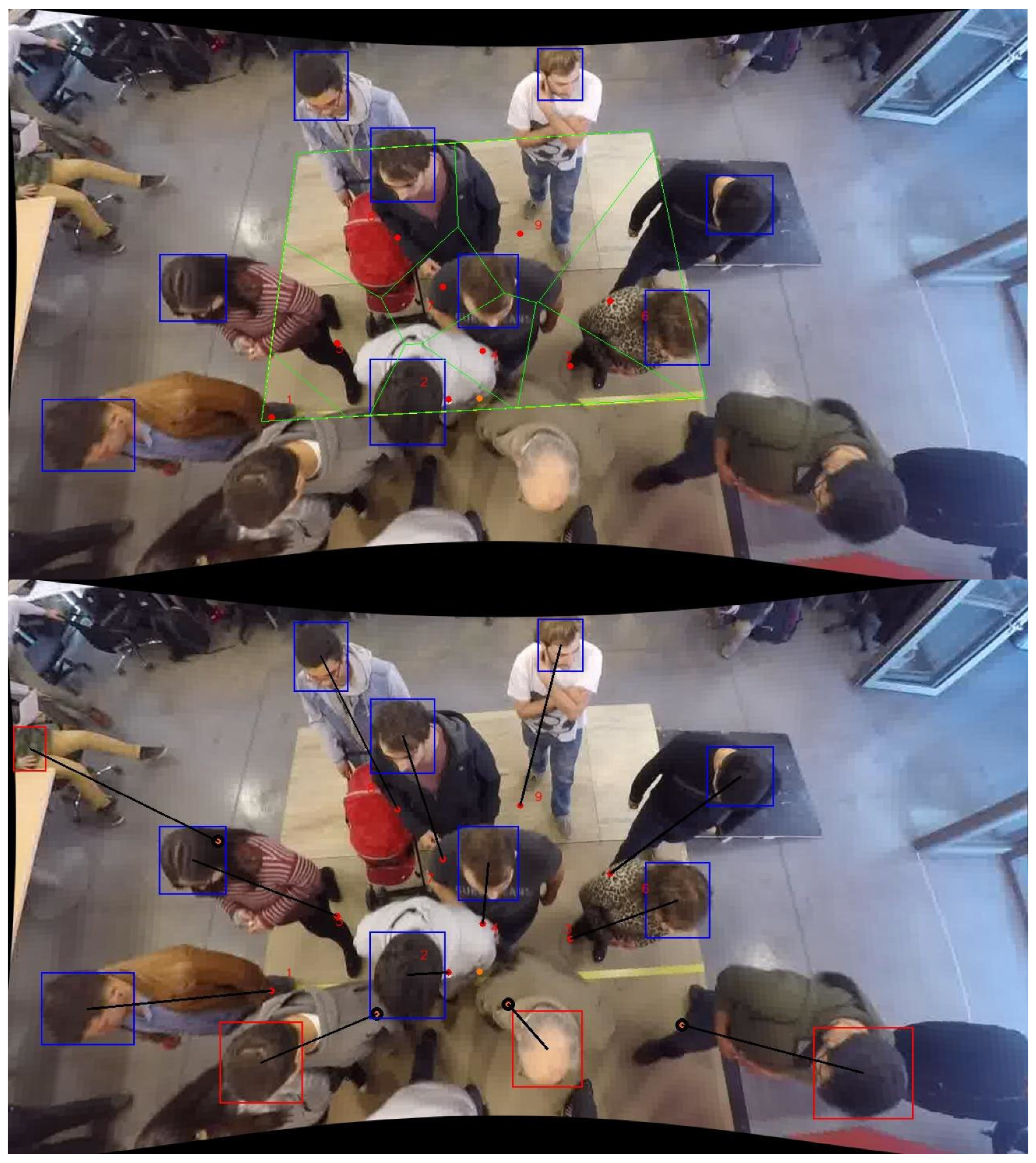
Figure 7 shows the boarding passengers who move from the platform to the carriage, while
Figure 8 presents the alighting process in which passengers move from the carriage to the platform. In both cases, the method is presented, considering the Voronoi polygons and the detections of passengers using the algorithm in the area of interest.
Figure 7 shows that nine passengers were detected on the platform (area of 6 m
2), i.e., the average density on the platform was 1.50 passengers/m
2 (i.e., average available space of 0.666 m
2/passenger). However, this average density (or available space per passenger) can be compared to the Voronoi polygons, in which each polygon represented an area used by each passenger (i.e., the inverse of the density). The results for each polygon are reported in
Table 4, in which the difference between the density using Voronoi polygons and Fruin’s Level of Service reached up to +301.6%. It is also important to notice that the variability of the density also presented a reduction in a range between 45.1% and 16.6%. This is caused because the Voronoi polygons represented the interaction between passengers in a more detailed manner. In other words, the Voronoi polygons represented the personal space occupied in the boarding process, while the average values of density using Fruin’s Level of Service are focused on the number of passengers on the whole platform. Therefore, if the Voronoi polygons are used, it is possible to identify where passengers are located and which part of the platform is more congested, thereby generating the data to support the need to redesign the platform–train interface which should have an improved LOS (Level of Service). In fact, the LOS is applied to the Voronoi polygons, in which
Table 4 shows that each boarding passenger represented a different LOS, reaching a value from A to F depending on the density of each polygon, which is affected by the number of passengers boarding on the platform.
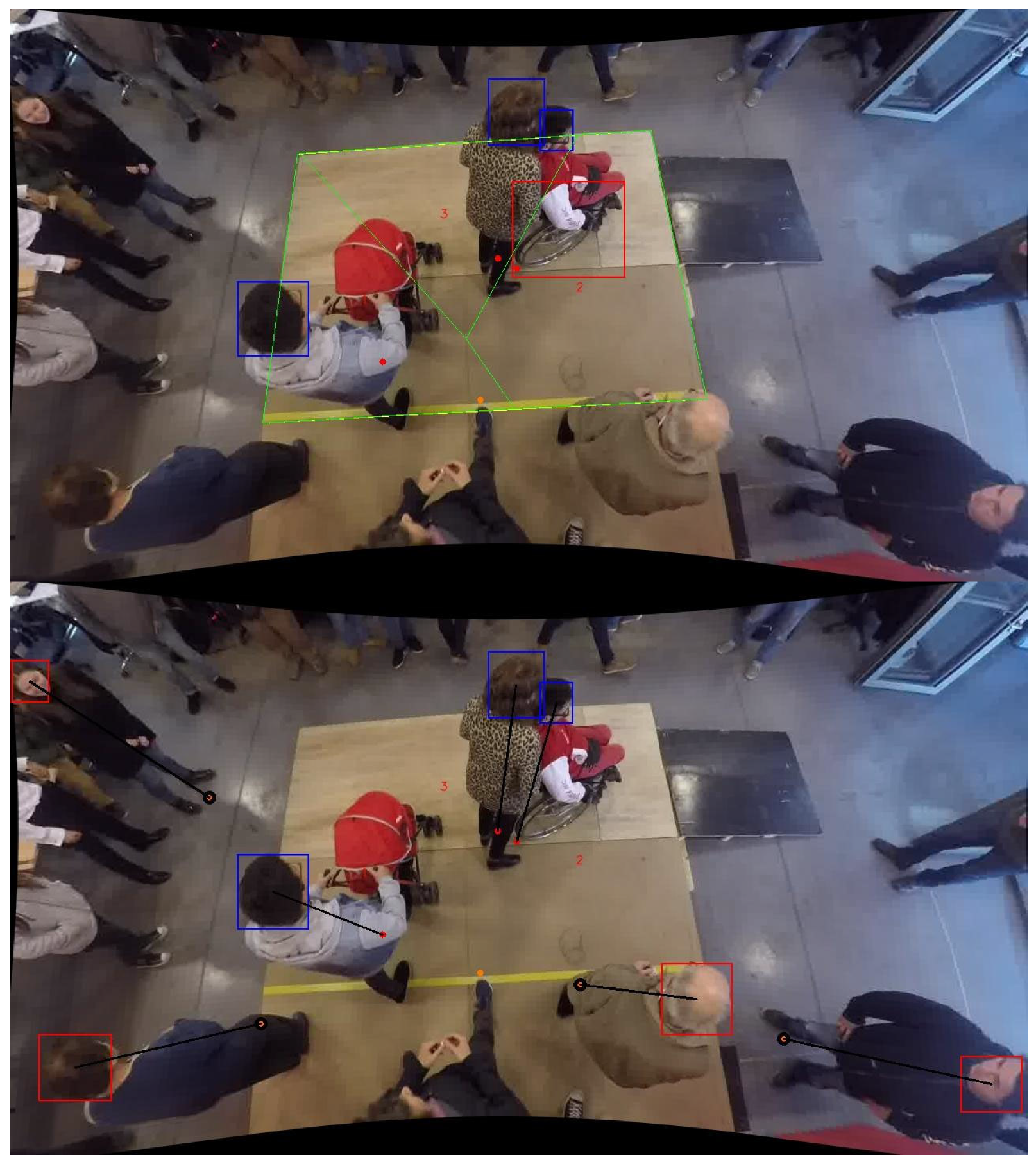
Similarly, in
Figure 8, three alighting passengers were detected on the platform and, therefore, the average density reached is equal to 0.50 passengers/m
2 (2.0 m
2/passenger). This average density (or available space per passenger) is different from the results obtained when using the Voronoi polygons.
Table 5 shows the difference between the average density using Fruin’s LOS and the Voronoi polygons, reaching a difference of up to +142.6%. It is important to mention that the variation also presented a negative variation of −48.8% in the case of polygon N°3, which is represented by the wheelchair passenger. It can also be noticed that polygon N°3 (corresponding to the passenger in a wheelchair) needed assistance from another passenger (polygon N°2). This means that both passengers (polygons N°2 and N°3) will need more space to move than a single passenger without reduced mobility.
Consequently, crowd management measures should be implemented, in which passengers could have some preferential space on the platform. For instance, some authors [
35,
49] have presented the use of waiting areas to facilitate the boarding and alighting processes, which will be explored in future experiments (see
Figure 9).
5. Conclusions
The study of the density of passengers on the platform is essential to determine the normal functioning of the platform–train interface (PTI). Therefore, this allows us to study which part of the PTI is more congested so that some crowd management measures for a station can be implemented (e.g., implementation of waiting areas on the platform).
The implementation of crowd management measures can be used by transport planners to provide certainty to passengers that the train will not stay at the platform for additional time when a crowded situation is reached. In addition, it can be used to identify when the platform needs to be redesigned to reduce the interaction between passengers boarding and alighting.
Nowadays, these crowd management measures and other design recommendations are also used to keep passengers safe due to COVID-19. In the case of urban railways, the Fruin’s Level of Service (LOS) is used, in which an LOS = B is recommended to maintain a social distance of at least 1.0 m between passengers, i.e., between 0.9 and 1.1 passengers per square meter. Therefore, if a density of 1.1 or more passengers per square meter is reached at the PTI, a crowd management measure should then be implemented. The use of the Level of Service B as a recommendation for the PTI is based on passengers who have a breadth of 0.66 m and a body depth of 0.33 m. However, there is a lack of recommendations in the case of other types of passengers, such as Chilean wheelchair users, in which the passenger breadth is 0.8 m and the body depth is 1.2 m (or 1.3 m if the wheelchair user needs assistance from another passenger), which will be considered in future experiments at the laboratory facility.
In addition, the method can allow the identification of wheelchair users in high-density situations at the PTI who may need additional assistance. However, passengers with reduced mobility need more space to move and, therefore, the method could help identify which passengers need more space when using mobility aids.
For the development of the method, the use of computer vision was necessary through the training of neural networks and image processing. The algorithm is presented as a novelty compared to the calculation of the area available per passenger within a certain convex area. It is important to highlight that the use of Voronoi polygons was more representative of the interaction between passengers at the PTI than the average values of density used in Fruin’s LOS. However, one of the main drawbacks occurring in the developed technique is the use of a constant value for the height of passengers. The best case was presented for a height of 1.75 m, which reached the lowest error. This has an impact on the measurements when presenting a varied population. Further research will seek to progress the preparation of a technique capable of dispensing with the variable of height, or that can calculate it autonomously.
With respect to the experiments, the approach used presented an ideal opportunity to test “what if” scenarios, in which the boarding and alighting process was represented considering a mock-up of a train carriage and its adjacent platform. The objective was to represent the variation in one variable, “X”, considering the rest of the variables without change. Therefore, the effect of the “X” variable on the passenger’s space or density at the platform–train interface could be analyzed. In the case of the boarding process, the Voronoi polygons represented up to 300% variation compared to the average values of density using Fruin’s Level of Service. In the case of the alighting process, the variation reached up to 142% of the difference between both methods, considering the need of wheelchair users. As a next step, the density of existing stations will be considered using the Voronoi polygons to compare them with Fruin’s Level of Service.
Finally, it is expected that this technique can contribute to further studies and development in the transportation field, using techniques derived from artificial intelligence. The field is still very wide and presents the possibility of experimenting with real scenarios.


 ,
, 


