Compressive Strength Prediction of Lightweight Concrete: Machine Learning Models

Abstract

Concrete is the most commonly used construction material. The physical properties of concrete vary with the type of concrete, such as high and ultra-high-strength concrete, fibre-reinforced concrete, polymer-modified concrete, and lightweight concrete. The precise prediction of the properties of concrete is a problem due to the design code, which typically requires specific characteristics. The emergence of a new category of technology has motivated researchers to develop mechanical strength prediction models using Artificial Intelligence (AI). Empirical and statistical models have been extensively used. These models require a huge amount of laboratory data and still provide inaccurate results. Sometimes, these models cannot predict the properties of concrete due to complexity in the concrete mix design and curing conditions. To conquer such issues, AI models have been introduced as another approach for predicting the compressive strength and other properties of concrete. This article discusses machine learning algorithms, such as Gaussian Progress Regression (GPR), Support Vector Machine Regression (SVMR), Ensemble Learning (EL), and optimized GPR, SVMR, and EL, to predict the compressive strength of Lightweight Concrete (LWC). The simulation approaches of these trained models indicate that AI can provide accurate prediction models without undertaking extensive laboratory trials. Each model’s applicability and performance were rigorously reviewed and assessed. The findings revealed that the optimized GPR model (R = 0.9803) used in this study had the greatest accuracy. In addition, the optimized SVMR and GPR model showed good performance, with R-values 0.9777 and 0.9740, respectively. The proposed model is economic and efficient, and can be adopted by researchers and engineers to predict the compressive strength of LWC.

1. Introduction

Concrete is the world’s most popular artificial building material and comprises four simple ingredients: cement, water, coarse and fine aggregates. Fine and coarse aggregates make approximately 60−75% of the concrete volume, and significantly impact the concrete’s newly mixed and cured characteristics, mixing proportions, and economy. 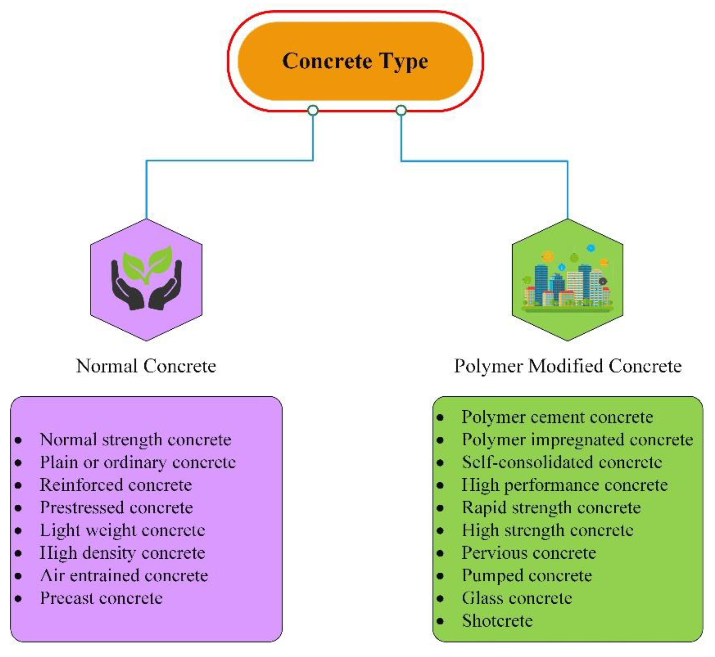The majority of the present research work has focused on using waste material in concrete production and improving the performance of the existing concrete mix considering the cost-effectiveness [1,2,3]. The commonly used concretes are of two types, normal concrete and polymer-modified concrete, as shown in Figure 1. The normal type of concrete contains normal-strength concrete, plain concrete, reinforced concrete, lightweight concrete, and air-entrained concrete, among other types, used in normal construction, such as small building. Polymer-modified concrete contains high-performance concrete, pervious concrete, self-consolidated concrete, and rapid-strength concrete, among other types, used in dams, tall chimneys, bridges, and multi-storey buildings. Lightweight concrete is extremely important for new construction, as well as repair and rehabilitation projects, among all kinds of concrete. The conventional technique ‘concrete jacketing’ is mainly used to strengthen/retrofit the concrete structures. However, increasing the weight, as well as a cross-section of the section, limit the use of this technique. Therefore, replacing the ordinary concrete with lightweight concrete with the same compressive strength can be an alternative solution.

Lightweight concrete is not a current concrete technology achievement. However, lightweight concrete was first used over 2000 years ago, and its innovation is still underway [4]. The “Port of Cosa, the Pantheon Dome, and the Coliseum” are three of the most prominent lightweight concrete buildings in the Mediterranean area [5]. They were all erected during the early Roman Empire. According to ACI 213, the term “lightweight aggregates (LWA) and lightweight concrete (LWC)” is defined “as the concrete which made up of lightweight coarse aggregates and normal weight fine aggregates with possibly some lightweight fine aggregates” [5]. Ordinary concrete is highly heavy self-weighted, with a total deadweight of around 2400–2500 kg/m³. LWC is 23–80% lighter than regular weight concrete, with a dry density ranging from 320 kg/m³ to 1920 kg/m³ [5]. Based on the density and strength parameters, the types of LWC are categorized in

Table 1. Types of lightweight concrete.

Type of LWC	Compressive Strength (N/mm2)	Density (kg/m3)
Low-density concrete	0.7–2.0	300–800
Moderate-strength concrete	7–14	800–1350
Structural concrete	17–63	1350–1920

. Low-density lightweight concrete has a variety of advantages in construction, including a reduced density, low thermal conductivity, low shrinkage, and excellent heat resistance, as well as a decrease in dead load, cheaper transportation costs, and a faster construction pace [6].

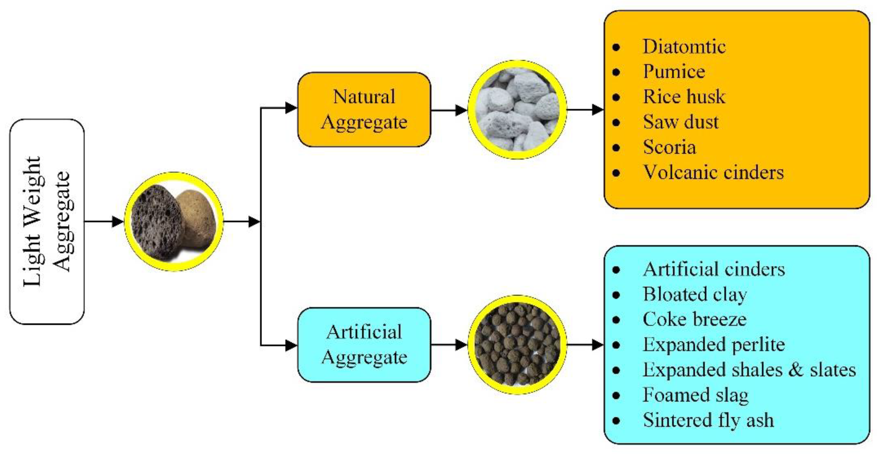
Several forms of LWA are now utilized to produce concrete lightweight, such as pumice perlite, expanded clays, shales, and other wastes, such as blended waste, agricultural waste, plastic or rubber, clay brick sintered fly ash aggregate, and oil palm shell. The commonly used methods are not considered in this study, as they are less efficient and consume more time to yield an output. In this manuscript, the most popular and efficient methods are used to determine the more accurate prediction in less time.

Compressive strength in concrete design, manufacture, and construction is regarded to be a basic performance criterion [7], and the 28-day compressive strength has been the most often utilized metric in many classical studies. The use of machine learning on laboratory data to estimate the 28-day compressive strength and other concrete parameters began in the early 2000s [8]. The prediction using ML models reduced the laboratory time, waste of constituents of concrete, and the cost. The various studies that have used ML to predict the compressive strength of a variety of concretes are described below.

Asteris et al. [9] used GPR, linear and non-linear multivariate adaptive regression splines (MARS-L and MARS-C), neural network (NN), and minimax probability machine regression (MPMR) to predict the compressive strength of concrete. The new hybrid model, called the hybrid ensemble model (HENSM), was used to compare the performance of four conventional models. Based on the experimental results, the HENSM model has the potential to be a new option for dealing with Conventional Machine Learning (CML) model overfitting difficulties and, therefore, may be used to forecast concrete compressive strength in a sustainable manner. Alshihri et al. [10] forecasted the compressive strength of concrete using an artificial neural network (ANN). In the ANN, two methods were utilized, called the feed-forward backpropagation (FFBP) and cascade correlation (CC) methods. Eight input variables—cement, water, w/c ratio, lightweight fine aggregate, sand, lightweight coarse aggregate, silica fume as a solution, superplasticizer, replacement of cement with silica fume, and curing period—were used to predict the compressive strength. The correlation coefficient of training and testing were 0.972 and 0.977 for BP, and 0.974 and 0.982 for CC. Compared to the BP technique, the CC neural network model predicted marginally more accurate outcomes and learned much faster.

Omran et al. [11] compared the data mining techniques to predict the compressive strength of environmentally friendly concrete. Four regression tree models and two ensemble methods were used in his study. The individual GPR model and its associated ensemble models had the greatest prediction accuracy in the comparison groups. Yaseen et al. [12] used four machine learning models, namely extreme learning machine (ELM), MARS, M5 Tree models, and SVR, to estimate the compressive strength of lightweight foamed concrete. Cement content, w/c ratio, oven-dry density, and foamed volume of aggregates were input factors for the prediction models. The findings demonstrated that the suggested ELM model improved the SVR, M5 Tree, and MARS models in terms of prediction accuracy. The ELM model may be used as an accurate data-driven method for forecasting the compressive strength of foamed concrete, avoiding the need for time-consuming trial batches to achieve the desired product quality.

Kandiri et al. [13] predicted the compressive strength of recycled aggregates using a modified ANN. The results of the ANN model were optimized with the help of the salp swarm algorithm (SSA), genetic algorithm (GA), and grasshopper optimization algorithm (GOA) techniques. The SSA-ANN model showed better accuracy compared to other models. Bui et al. [14] used a hybrid whale optimization algorithm (WOA)-ANN to estimate the compressive strength of concrete. Two other benchmark techniques, the dragonfly algorithm (DA) and ant colony optimization (ACO), were used to validate the accuracy of the model. The findings showed that the WOA-ANN outperformed the DA-ANN and ACO-ANN models. The accuracy of the WOA-ANN, GA-ANN, and ACO-ANN models were 89.76%, 82.09%, and 80%, respectively.

Sharafati et al. [15] predicted the compressive strength of hollow concrete prism with a bagging ensemble model. Three modelling scenarios based on distinct data divisions (i.e., 80–20%, 75–25%, and 70–30%) were used for the training and testing stages. The bagging regression (BGR) results were compared with the SVR and decision tree regression (DTR) models. The BGR model achieved a low root mean square error (RMSE = 1.51 MPa) in the testing phase while employing the 80–20% data division scenario, whereas the DTR and SVR models achieved RMSE = 2.55 and 2.33 MPa, respectively. Xu et al. [16] used ML to forecast the compressive strength of ready-mix concrete. Random forest (RF) was used as the modelling technique to predict the compressive strength from the selected influential elements after GA was used to find the most relevant influential factors for compressive strength modeming. A case study was used to assess the efficiency of the suggested model, and the highest R-value was 0.9821 and lowest MAPE and delta values were 0.0394 and 0.395, respectively, showing that the model can produce precise and dependable outcomes.

The work in this research article is categorized into five parts. Section 2 provides a detailed overview of the formation of lightweight concrete and defines the lightweight aggregate. Section 3 is related to the collection of lightweight aggregate from the literature and the processing of the raw data. Section 4 describes the overview of the selected machine learning algorithms. The results and discussions are mentioned in Section 5, and the conclusion of the article is explained in Section 5.

2. Formation of Lightweight Concrete

2.1. Lightweight Aggregate (LWA)

Lightweight concrete is mainly formed using lightweight aggregates, as shown in Figure 2. The ASTM standard covers two types of lightweight aggregate specifications: (i) aggregates manufacturing by pelletizing, expanding, or sintering such as shale, diatomite, etc., and (ii) aggregates manufacturing processing natural materials such as tuff, pumice, etc., as shown in Figure 2. Furthermore, the ASTM C331M lists lightweight “aggregates made out of final coal or coke products” [17]. Details on the various LWA classes, their characteristics, and the normal production procedures for additional study are provided in the literature [18,19,20]. To differentiate between standard weight aggregate and LWA, the specification of aggregate characteristics, particularly density, is the crucial parameter. Upper limitations for the loose bulk density are given by ASTM C330M and ASTM C331M, which are 1120 kg/m³ for fine lightweight aggregate, 880 kg/m³ for coarse lightweight aggregate, and 1040 kg/m³ for a mix of fine and coarse lightweight aggregate. According to the ASTM, the compressive strength and split tensile requirements for lightweight aggregate are shown in Figure 3.

2.2. Lightweight Concrete (LWC)

The structural designer appreciates a reduction in concrete density since concrete weight typically accounts for more than half of the dead load in a structure. “The lightweight structural concrete made with the aggregates defined in ASTM C 330. The concrete has a minimum 28-day compressive strength of 17 N/mm², an equilibrium density between 1120 and 1920 kg/m³, and consists entirely of lightweight aggregate or a combination of lightweight and normal-density aggregate”. The use of LWC is generally justified by a desire to save money on a project, enhance functionality, or a combination of the two. When contemplating lightweight concrete, estimating the overall cost of a project is important because the cost of a cubic meter is generally more than a comparable unit of regular concrete, as mentioned in ACI 213.

Manufacturing companies manufacture structural-grade lightweight aggregates from raw materials such as appropriate fly ash, shales, slates, clays, or blast-furnace slag. The growing usage of processed lightweight aggregates is a good example of environmental planning and sustainability. These products reduce construction industry demands on scarce natural gravel, stone, and sands resources by requiring less transportation and the use of minerals that have limited structural uses in their natural condition.

3. Collection of LWC Data

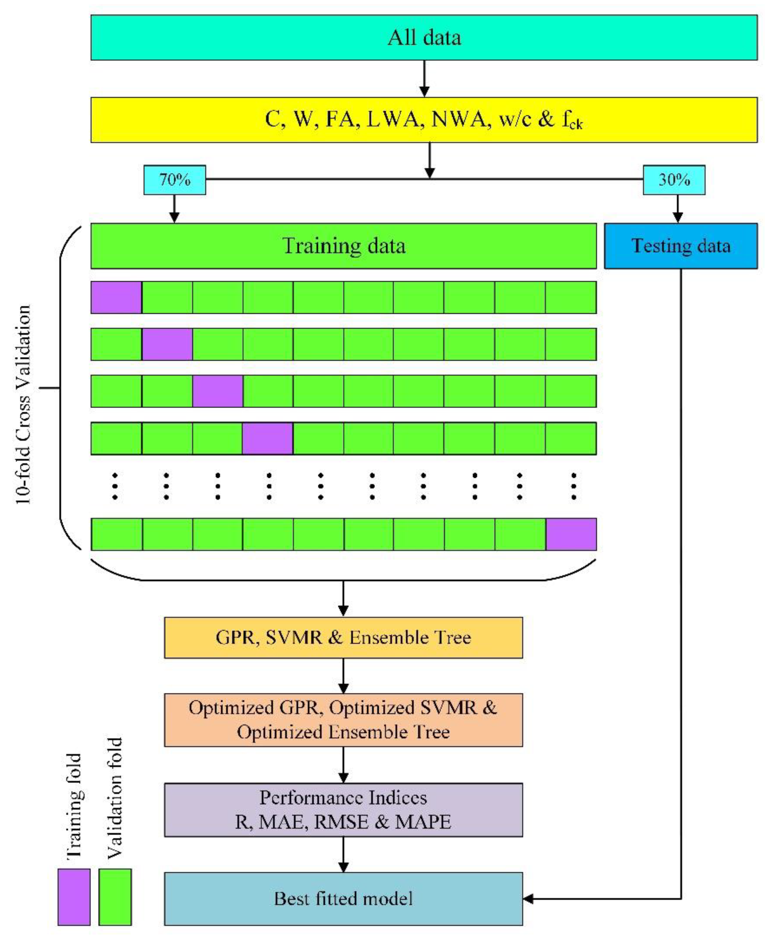
To build the models for predicting compressive strength in this study, a complete database of 194 different experimental records of concretes was compiled from the literature [21,22,23,24,25,26,27,28,29,30,31,32,33,34,35,36,37,38,39,40]. In this study, only one target parameter was considered, that is, the compressive strength of concrete (f_ck). The input parameters used in this article are the basic constituents of the concrete mix, such as cement (C), water content (W), fine aggregate (FA), normal weight coarse aggregate (NWCA), lightweight coarse aggregate (LWCA), and water-cement ratio (w/c). The only one output parameter is considered that is compressive strength (f_ck) of LWC.. The ranges of these parameters are from 208.57 to 640 Kg/m³, from 93.86 to 251 Kg/m³, from 150 to 1096 Kg/m³, from 0 to 1083 Kg/m³, from 0 to 730 Kg/m³, from 0.25 to 0.55, and from 19 to 96 N/mm², respectively, as shown in

Table 2. The input and output parameters needed to predict the compressive strength of LWC are described using descriptive statistics.

Parameters	Symbol	Unit	Mean	Min.	Max.	Std.	Skewness	Kurtosis	Type
Concrete Parameters	w/c	-	0.39	0.25	0.55	0.073	0.3971	2.67	Input
	C	Kg/m3	460.35	208.57	640	73.36	−0.0889	4.31
	W	Kg/m3	184.63	93.86	251	26.88	0.0849	3.41
	FA	Kg/m3	661.76	150	1096	280.46	−0.4924	2.29
	LWCA	Kg/m3	366.04	0	730	221.25	−0.3627	2.12
	NWCA	Kg/m3	298.23	0	1083	404.24	0.7953	1.89
	fck	N/mm2	39.43	16	96	14.38	1.75	6.95	Output

.

The original test database was filtered according to the following principles to increase the database’s dependability: (a) One test dataset should be removed from a dataset with the same test parameters if the goal value compressive strength differs by more than 15% from the other test data and the other test data points differ by less than 15%. (b) If the difference between any two test data points in a set of data under the identical test conditions is greater than 15%, the entire data group must be discarded. The 194 test data points were eventually reduced to 120 remaining data points using the aforementioned data filtering procedures. Table 2 shows the descriptive statistics of the collected database.

Data normalization was performed before processing the data in the machine learning algorithms. The normalization process reduces the undesired feature scaling effects and provides higher computational stability. All parameters were normalized in the range from 0 to 0.9 using Equation (1) [41].

$$y^{*}=0.9\times \frac{\left(y-y_{min}\right)}{y_{max}-y_{min}}$$

(1)

where y* is the value to be normalized, y is the original value in the dataset, y_max is the maximum value in the desired dataset, and y_min is the minimum value in the desired dataset.

Six frequently used performance indices such as correlation coefficient (R), root mean squared error (RMSE), mean absolute error (MAE), mean absolute percentage error (MAPE) [42], a20-index [43], and Nash-Sutcliffe (NS) efficiency index [44]—are used to analyse the performance of selected machine learning models. R and NS values closer to one indicate a better relationship between the desired result, but R values greater than 0.85 indicate a substantial relationship. The lower the values of MAPE, RMSE, and MAE, the greater the performance of the selected models. 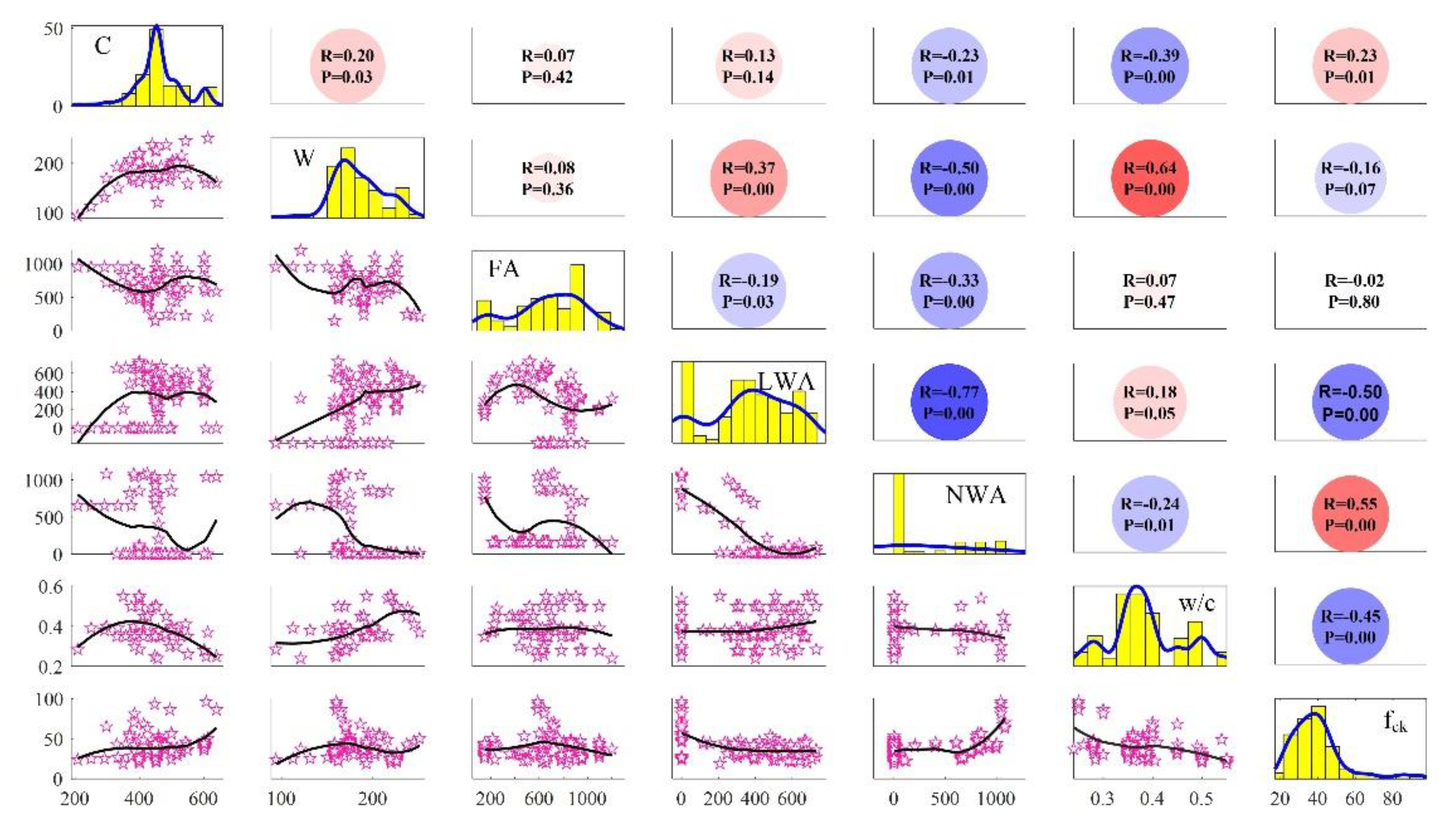Equations (2)–(7) [42,43,44] show the relevant expressions of the R, MAE, MAPE, RMSE, NS, and a20-index, respectively. These indices’ relevant expressions are given in Equations (2)–(7). The scatterplot matrix of the collected data is shown in Figure 4. Figure 4 shows the correlation coefficient of each input and output value, as well as the correlation with each variable. A probability (p-value) is assigned to the correlation coefficients, indicating the likelihood that the link between the two variables is zero (null hypotheses; no relationship). Strong correlations have low p-values because the chances of the correlations not being related are exceedingly small.

$$R=\frac{{{\displaystyle \sum }}_{i=1}^N\left(E_i-\overline{x}\right)\left(P_i-\overline{P}\right)}{\sqrt{{{\displaystyle \sum }}_{i=1}^N{\left(E_i-\overline{E}\right)}^2{\left(P_i-\overline{P}\right)}^2}}$$

(2)

$$MAE=\frac{1}{N} {\displaystyle \sum }_{i=1}^N\left|E_i-P_i\right|$$

(3)

$$MAPE=\frac{1}{N} {{\displaystyle \sum }}_{I=1}^N\left|\frac{E_i-P_i }{E_i}\right|\times 100$$

(4)

$$RMSE=\sqrt{\frac{{{\displaystyle \sum }}_{i=1}^N{\left(E_i-P_i\right)}^2}{N}}$$

(5)

$$NS=1-\frac{{{\displaystyle \sum }}_{i=1}^N{\left(E_i-P_i\right)}^2}{{{\displaystyle \sum }}_{i=1}^N{\left(E_i-\overline{P_i}\right)}^2}$$

(6)

$$a20-index=\frac{m20}{N}$$

(7)

where N is the number of samples in the datasets, $E_i$ is the experimental value at the ith level, $\overline{E}$ is the mean of experimental values, $P_i$ is the predicted value at the ith level, and $\overline{P}$ is the mean of predicted values. m20 is the number of samples with values rate measured/predicted values (range between 0.8 and 1.2).

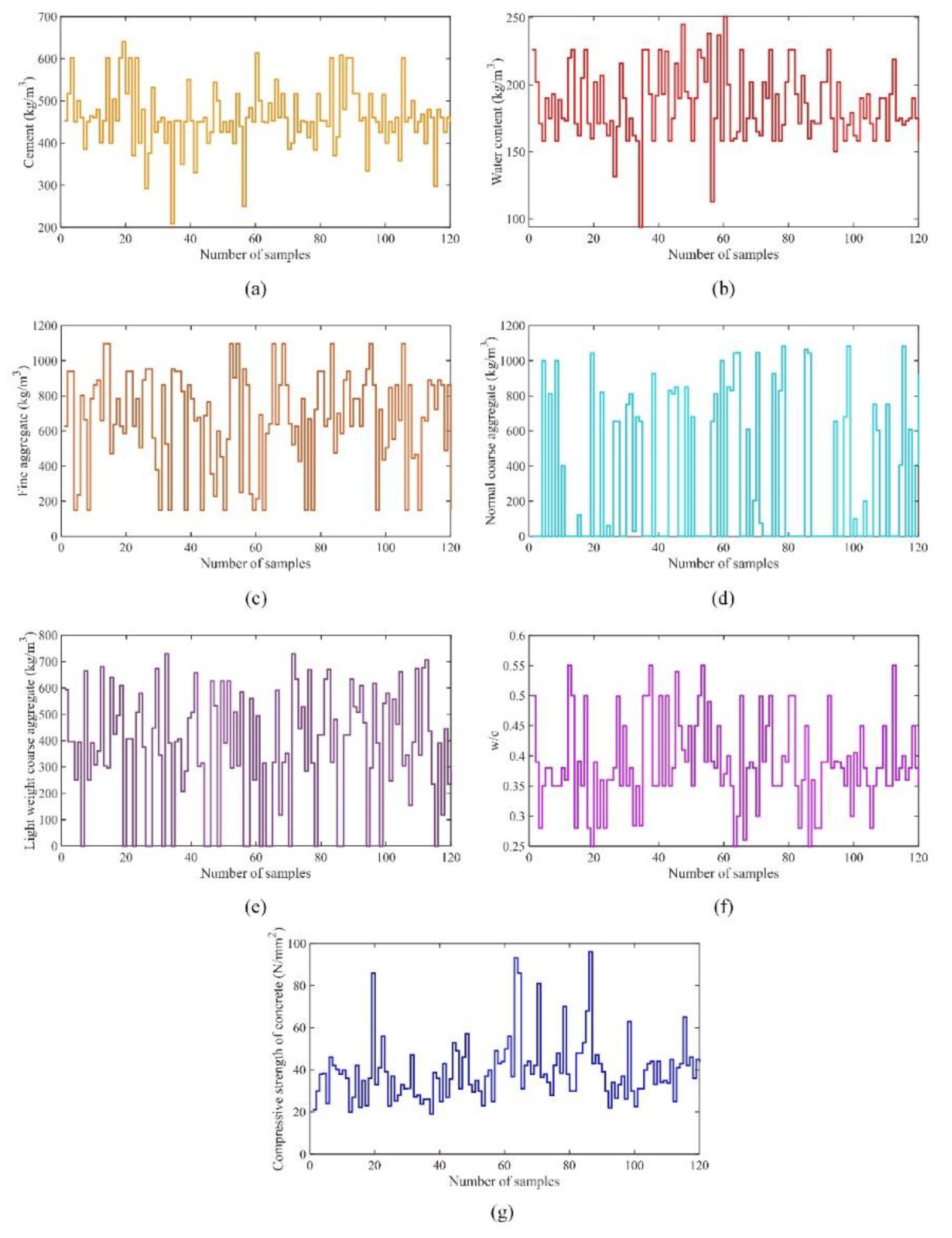
Figure 5 shows the distribution of the input and output parameters for each dataset. Figure 5a shows the distribution of cement content with the number of samples in the dataset, Figure 5b shows the distribution of water content with the number of samples in the dataset, Figure 5c shows the distribution of fine aggregate with the number of samples in the dataset, Figure 5d shows the distribution of normal weight coarse aggregate with the number of samples in the dataset, Figure 5e shows the distribution of lightweight coarse aggregate with the number of samples in the dataset, Figure 5f shows the distribution of the water-cement ratio with the number of samples in the dataset, and Figure 5g shows the distribution of the compressive strength of concrete with the number of samples in the dataset.

4. Overview of Machine Learning Methods

This section provides an overview of the methods used to construct the prediction models for the compressive strength of concrete incorporating machine learning algorithms. Artificial intelligence (AI) is subdivided into machine learning (ML), which focuses on the creation of prediction algorithms. This branch of artificial intelligence enables computers to carry out difficult and sophisticated tasks that were previously inaccessible to machines. These algorithms developed the capacity to learn patterns from data rather than relying on people to train them. These algorithms are built on training, allowing the computer to learn the properties/features that ideally compose the dataset for the given problem. Then, the computer interprets this knowledge to create more accessible datasets. Three ML algorithms, namely GPR, SVMR, and EL, are described below.

4.1. Gaussian Processes Regression

The concept of the GPR model is named after Carl Friedrich Gauss, as it is based on the notion of Gaussian distribution (normal distribution) [42]. GPR is a real-valued variable-based approach on Bayesian inference [45]. It is a non-parametric prediction model for a given dataset function. GPR is defined as D = {(x_i, t_i), i = 1, 2,..., N}, where x_i is an input variable and t_i is a target variable [41]. A distribution function, called “Gaussian process regression,” can be as expressed as shown in Equation (8), used for the Bayesian regression.

$$P\left(f|D\right)=\frac{p\left(f\right)p(d|f)}{p\left(D\right)}$$

(8)

The primary function in GPR, called k(x, x′), is the covariance function. The covariance function can be performed best, as shown in Equation (9).

$$k\left(x,x\prime \right)={\sigma }_f^{2}exp\left\{-\frac{1}{2}\left(\frac{x_i-x_j}{l^2}\right)\right\}$$

(9)

where l is the scale length and ${\sigma }_f^2$ is the maximum permissible variance. Equation (10) shows the output of the latent function.

$$y=f\left(x\right)+\epsilon$$

(10)

where ε is the Gaussian noise and (x) is the latent function. In GPR, the latent function is regarded as a random variable. For the aforementioned covariance function, if the difference between x and x′ approaches zero, the (x) function is close to the actual function (x)′. The above equation may be rewritten as follows by adding the noise values.

$$k\left(x,x\prime \right)={\sigma }_f^{2}exp\left\{-\frac{1}{2}\left(\frac{x_i-x_j}{l^2}\right)\right\}+{\sigma }_n^2 \delta \left(x,x\prime \right)$$

(11)

where, δ(x, x′) is Kronecker delta function and ${\sigma }_n^2$ is the variance of n observations. The forecasted function can be written as:

$$y=f\left(x\right)+N\left(0,{\sigma }_n^2\right)$$

(12)

The covariance or kernel function (x,′) is expressed in Equation (13).

$$K=\left[\begin{array}{cccc}k\left(x_1,x_2\right)& k\left(x_1,x_2\right)& \dots & k\left(x_1,x_n\right)\\ k\left(x_2,x_1\right)& k\left(x_2,x_2\right)& \dots & k\left(x_2,x_n\right)\\ ⋮& ⋮& & ⋮\\ k\left(x_n,x_1\right)& k\left(x_n,x_2\right)& \dots & k\left(x_n,x_n\right)\end{array}\right]$$

(13)

4.2. Support Vector Machines Regression

Vapnik et al. [46] created SVM, a supervised machine learning model for solving high-dimensional problems. Depending on the data, this approach may be used to solve regression or classification issues [47,48]. “A hyperplane is used in SVM to map a set of training samples representing points in space to a multidimensional feature space”. SVM offers several benefits, including the capacity to “handle high-dimensional space data,” “situations with a greater number of dimensions than sample count,” “memory efficiency,” and the flexibility to model the decision function using a variety of kernel functions. The goal of applying this technique is to predict the target variables using the input data, which include K-dimensional x_i patterns and y_i findings, as well as training and test data. When combined with core functions, SVM is quite effective. As a result, a nonlinear optimal boundary in the input space corresponds to the extreme plane defining SVM.

The SVM is a well-known approach based on the statistical learning theory that takes full use of the notion of structural risk reduction rather than the standard empirical risk minimization employed in older methods to assure the generalization capacity of the regression model [49]. The cubic SVM method was proven to be more accurate than the other techniques in the experiments using all sub-methods (linear and quadratic SVM) of SVM. As a result, in the current work, a cubic SVM was utilized to forecast the compressive strength of lightweight concrete. The SVM model’s sketch map is shown in Figure 6.

The following regression function may be used to define the nonlinear input-output connection in the SVM model if the ith sample contains a D-dimensional input vector x_i $ϵ$ R^D and a scalar output y_i $ϵ$ R.

$$f\left(x_i\right)={\omega }^T\varnothing \left(x_i\right)+b, i=1, 2, \dots i$$

(14)

where $f\left(x_i\right)$ represents the forecasted values, $\varnothing \left(x_i\right)$ is the nonlinear mapping function, and the optimized parameters are ω and b.

For the training dataset with l samples, the ϑ-SVM optimization model can be expressed as follows:

$$\{\begin{array}{c}minR\left(\omega ,\xi ,{\xi }^{*},\epsilon \right)=\frac{1}{2}{||\omega ||}^2+C\left[\vartheta \epsilon +\frac{1}{l}{\displaystyle \sum }_{i=1}^l\left({\xi }_i+{\xi }_i^{*}\right)\right]\\ subject to: y_i-{\omega }^T\phi \left(x_i\right)-b \le \epsilon +{\xi }_i\\ \frac{{\omega }^T\phi \left(x_i\right)+b-y_i\le \epsilon +{\xi }_i}{{\xi }^{*}, \epsilon \ge 0}\end{array}$$

(15)

where C is the parameter used to stabilize the model complexity and empirical risk term ${||\omega ||}^2$, and ${\xi }_i^{*}$ denotes the distance and is called a slack variable. The Lagrange multipliers technique is used to solve the dual optimization problem as expressed in Equation (16).

$$\{\begin{array}{c}maxR\left(a_i,a_i^{*}\right)= {\displaystyle \sum _{i=1}^l}{y}_i\left(a_i,a_i^{*}\right)- \frac{1}{2}{\displaystyle \sum _{i=1}^l}{\displaystyle \sum _{j=1}^l}\left(a_i-a_i^{*}\right)\left(a_j-a_j^{*}\right) K\left(x_i,x_i^{*}\right)\\ subject to: {\displaystyle \sum _{i=1}^l}\left(a_i-a_i^{*}\right)=0, 0\le a_i, a_i^{*}\le C/l\\ {\displaystyle \sum _{i=1}^l}(a_i+a_i^{*})\le C.v\end{array}$$

(16)

where kernel functions are denoted by K(x_i, x_j), and the non-negative Lagrange multipliers are represented by a_i and $a_i^{*}$. Equation (17) expresses the regression for an unknown input vector x.

$$f\left(x\right)={\displaystyle \sum }_{i=1}^l\left(a_i-a_i^{*}\right)\times K\left(x,x_i\right)+b$$

(17)

4.3. Ensembles Learning

In several research and commercial challenges involved in many industrial domains, EL algorithms have been shown to have great generalization capacity. A typical EL method with n ML models may be written as follows [50]:

$$F^{EL}\left(x\right)={{\displaystyle \sum }}_{i=1}^n{F}_i^{ML}\left(x\right)$$

(18)

where x is the input parameters, $F^{EL}\left(x\right)$ is the final mode established through the EL algorithm, and $F_i^{ML}\left(x\right)$ is the selected ML algorithm, called the basis model.

Ensemble techniques train several machine learning algorithms to arrive at a final conclusion. EL’s are based on human behaviour, which assumes that each problem can be solved by gathering and implementing the opinions of a number of experts [51]. Based on these differing viewpoints, a decision is made. When compared to employing a single classifier, ELs provide superior results.

There are two main approaches for the construction of basic models in the EL algorithm. Boosting techniques are algorithms that construct the base ML models in a sequential manner. Each basis model in the boosting method (BM) is strongly dependent on one of the basis models $F_i^{ML}\left(x\right)$, and the training is regulated by the former “basis model” $F_{i-1}^{ML}\left(x\right)$. Bagging approaches are those that train the “basis models” in a parallel framework, with each basis model $F_i^{ML}\left(x\right)$ being completely independent [52]. The boosting approach would significantly enhance a model’s prediction variance and bias as a consequence of several methods, but the bagging method could simply raise the stability of a model by lowering the variance. Many research articles have indicated that the boosting method beats the bagging method in terms of prediction accuracy.

5. Results and Analysis

5.1. Implementation of Machine Learning Alogthims to Predict the Compressive Strength

Based on the training process of the ML algorithms, the data were divided into two parts. To avoid the overfitting phenomenon, the splitting ratio of the two sets was adjusted to 7 ratios 3, where 70% (84 samples) of the data was used in the training process and the other 30% (36 samples) of the data was utilized as testing data, as shown in Figure 7. To validate the results of the ML algorithms, cross-validation with the 10-fold method was used. In the 10-fold cross-validation method, the dataset was split into 10 subsets. Each subset was for the validation process, with the remaining 9 subsets being utilized for training inside the training stage.

5.2. Results of ML Algorithms

5.2.1. GPR Model

In the GPR method, the Matern 5/2 GPR algorithm was found to be more precise than the rest of the methods. The properties of the selected GPR are tabulated in

Table 3. Selected properties of the Matern 5/2 GPR model.

Parameter	Value
Basic function	Constant
Use isotropic kernel	Yes
Kernel scale	3.12
Signal standard deviation	0.0785
Sigma	0.0785
Optimize numeric parameters	Yes

. In the training stage, the GPR model predicted the compressive strength values practically accurately. However, there was a little difference in the testing stage. The GPR model’s prediction accuracy (R = 0.9931, MAE = 1.4395, MAPE = 3.9752, and RMSE = 1.8262 in the training phase, R = 0.8639, MAE = 4.0267, MAPE = 11.3444, and RMSE = 5.3077 in the testing phase) demonstrates the model’s generalisation capability in both phases. In Figure 8, a scatterplot shows the experimental and forecasted values of the compressive strength of LWC for the training and testing datasets. The details of the other performance indices are tabulated in

Table 4. Statistical analysis results of different models.

Model	R	MAE	MAPE	RMSE	NS	a20-Index
GPR	0.974	2.1023	5.8632	3.2603	0.9477	0.9580
SVMR	0.9647	2.8526	7.8439	4.1512	0.7566	0.8750
EL	0.9571	3.3334	8.6391	4.4732	0.9020	0.8500
Optimized GPR	0.9803	1.9909	5.5676	2.8294	0.9606	0.9670
Optimized SVMR	0.9777	2.5106	7.0123	3.7741	0.9299	0.9500
Optimized EL	0.9621	3.1132	8.5132	3.9666	0.9227	0.9500

.

Further, the GPR model was optimized using the parameters shown in

Table 5. Selected properties of the optimized GPR model.

Parameter	Value
Basic function	Constant
Kernel function	Isotropic Rational Quadratic
Kernel scale	0.37139
Signal standard deviation	0.12845
Sigma	0.01588
Optimize numeric parameters	Yes

. The plot between the minimum mean square error (MSE) and the number of iterations for normalized values is shown in Figure 9. The prediction accuracy of the optimized GPR model for the training and testing phase was R = 0.9933, MAE = 1.4063, MAPE = 3.8953, RMSE = 1.7982, and R = 0.8915, MAE = 3.6880, MAPE = 10.4227, RMSE = 4.4002, respectively, as shown in

Table 6. Details of each model’s performance indexes during the training and testing stage.

Model	R			MAE			MAPE			RMSE
	Training	Testing	All	Training	Testing	All	Training	Testing	All	Training	Testing	All
GPR	0.9931	0.8639	0.9740	1.4395	4.0267	2.1023	3.9752	11.3444	5.8632	1.8262	5.3077	3.2603
SVMR	0.9784	0.8799	0.9647	2.3648	4.2689	2.8526	6.4588	11.8652	7.8439	1.5979	5.6277	4.1512
EL	0.9653	0.9163	0.9571	3.3133	3.3941	3.3334	8.3943	9.3498	8.6391	4.5923	3.8653	4.4732
Optimized GPR	0.9933	0.8915	0.9803	1.4063	3.6880	1.9909	3.8953	10.4227	5.5676	1.7982	4.4002	2.8295
Optimized SVMR	0.9947	0.8882	0.9777	1.2962	6.0363	2.5106	3.6952	16.6425	7.0123	3.2988	4.6111	3.7742
Optimized EL	0.9764	0.9051	0.9621	2.8698	3.8196	3.1132	7.8365	10.4778	8.5132	3.5887	4.6127	3.9666

. The comparison between the experimental and forecasted values is shown in Figure 10.

5.2.2. SVMR Model

In all trained SVMR models, the cubic SVMR model outperformed the other models. The parameters used to train the desired SVMR model are presented in

Table 7. Selected properties of the cubic SVMR model.

Parameter	Value
Box constraint	0.1323
Epsilon	0.1204
Kernel scale	1

. The SVMR model’s prediction accuracy (R = 0.9784, MAE = 2.3648, MAPE = 6.4588, and RMSE = 1.5979 in the training phase, R = 0.8799, MAE = 4.2689, MAPE = 11.8652, and RMSE = 5.6277 in the testing phase) demonstrates the model’s general capability in both phases. Figure 11 shows the training and testing data scatterplot between the experimental and forecasted values.

The SVMR model was optimized using

Table 8. Selected properties of the optimized SVMR model.

Parameter	Value
Kernel function	Cubic
Box constraint	0.0018365
Epsilon	0.00012396
Kernel scale	1

parameters. The accuracy of the optimized SVMR model was 1.67% higher than the conventional SVMR model. The plot between the minimum mean square error (MSE) and a number of iterations for normalized values is shown in Figure 12. In terms of R, MAE, MAPE, and RMSE, the prediction accuracy of the optimized SVMR model for the training and testing data was 0.9947, 1.2962, 3.6952, 3.2988, and 0.8882, 6.0363, 16.6425, 4.6111, respectively. The comparison between the experimental and forecasted values of the training and testing dataset is shown in Figure 13.

5.2.3. EL Model

Both boosted and bagged trees models were trained in the EL algorithm, and it was found that the boosted trees model performed well. The prediction accuracy of the EL model (R = 0.9653, MAE = 3.3133, MAPE = 8.3943, and RMSE = 4.5923 in the training phase, R = 0.9163, MAE = 3.3941, MAPE = 9.3498, and RMSE = 3.8653 in testing phase) demonstrates the model’s general capability in both phases, using

Table 9. Selected properties of the boosted EL model.

Parameter	Value
Leaf size	10
Number of learners	42
Learning rate	0.1

parameters. In Figure 14, a scatterplot depicts the comparison between the experimental and forecasted values of the compressive strength of LWC for the training and testing datasets. The details of the other performance indices are tabulated in Table 4.

Further, the EL model was optimized using the parameters shown in

Table 10. Selected properties of the optimized EL model.

Parameter	Value
Minimum leaf size	1
Number of learners	499
Number of predictors to sample	3

. The plot between the minimum mean square error (MSE) and the number of iterations for normalized values is shown in Figure 15. The prediction accuracy of the optimized EL model for training and testing phase was R = 0.9764, MAE = 2.8698, MAPE = 7.8365, RMSE = 3.5887, and R = 0.9051, MAE = 2.8698, MAPE = 10.4778, RMSE = 4.6127, respectively, as shown in Table 5. The comparison between the experimental and predicted values is shown in Figure 16.

5.3. Comparison of Results of ML Models

The performance of the optimized GPR model is excellent among all the models based on the performance indices. The correlation coefficient of the optimized GPR model was 0.65%, 1.62%, 2.42%, 0.27%, and 1.89% higher than the GPR, SVMR, EL, optimized SVMR, and optimized EL models, respectively. Similarly, the optimized GPR model had the highest NS and a-20 index among the other models. The MAE-value of the optimized GPR model was 1.9909, which was 5.3%, 30.2%, 40.27%, 20.7%, and 36.05% lower than the GPR, SVMR, EL, optimized SVMR, and optimized EL models, respectively. Similarly, the MAPE and RMSE values of the optimized GPR model were the lowest compared to other models, with values of 5.5676 and 2.8298, respectively. The performance of the rest of the models is given in decreasing order: GPR, optimized SVM, SVM, optimized EL, and EL models.

Figure 17 illustrates the experimental and predicted compressive strength calculated by the GPR, SVMR, EL, and optimized GPR, SVMR, and EL. The error between the experimental and predicted values is examined in Figure 17. Different ML algorithms were used to recognize the pattern embedded in the experimental data, and variation in the predicted datasets was compared with the ML models. The greater difference between the experimental dataset and ML algorithms indicates higher errors. The dark blue dotted lines reflect the experimental values in each graph, while the red lines show the predicted values. The sky-blue circles beneath these lines show their errors.

6. Conclusions

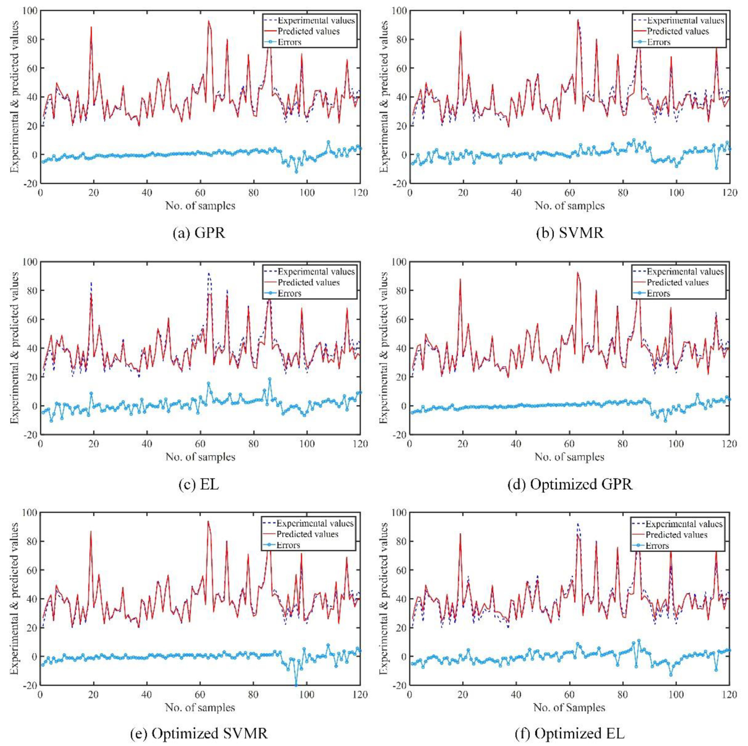
The purpose of this study was to compare the different ML-based prediction models used for predicting the compressive strength of LWC based on the dataset characteristics. The compressive strength of LWA was predicted using various algorithms, such as GPR, SVMR, EL, optimized GPR, optimized SVMR, and optimized EL. In total, 120 datasets were used in this study, which were taken from the literature. The prediction of the lightweight concrete f_ck was predicted using all the concrete parameters (C, W, FA, LWCA, NWCA, w/c) provided in the database. R, RMSE, MAE, MAPE, NS, and a20-index statistical indices were used to evaluate and compare the prediction accuracy of different models. The following conclusions were drawn:

• The conventional and optimized machine models used for forecasting the compressive strength of LWC performed well.
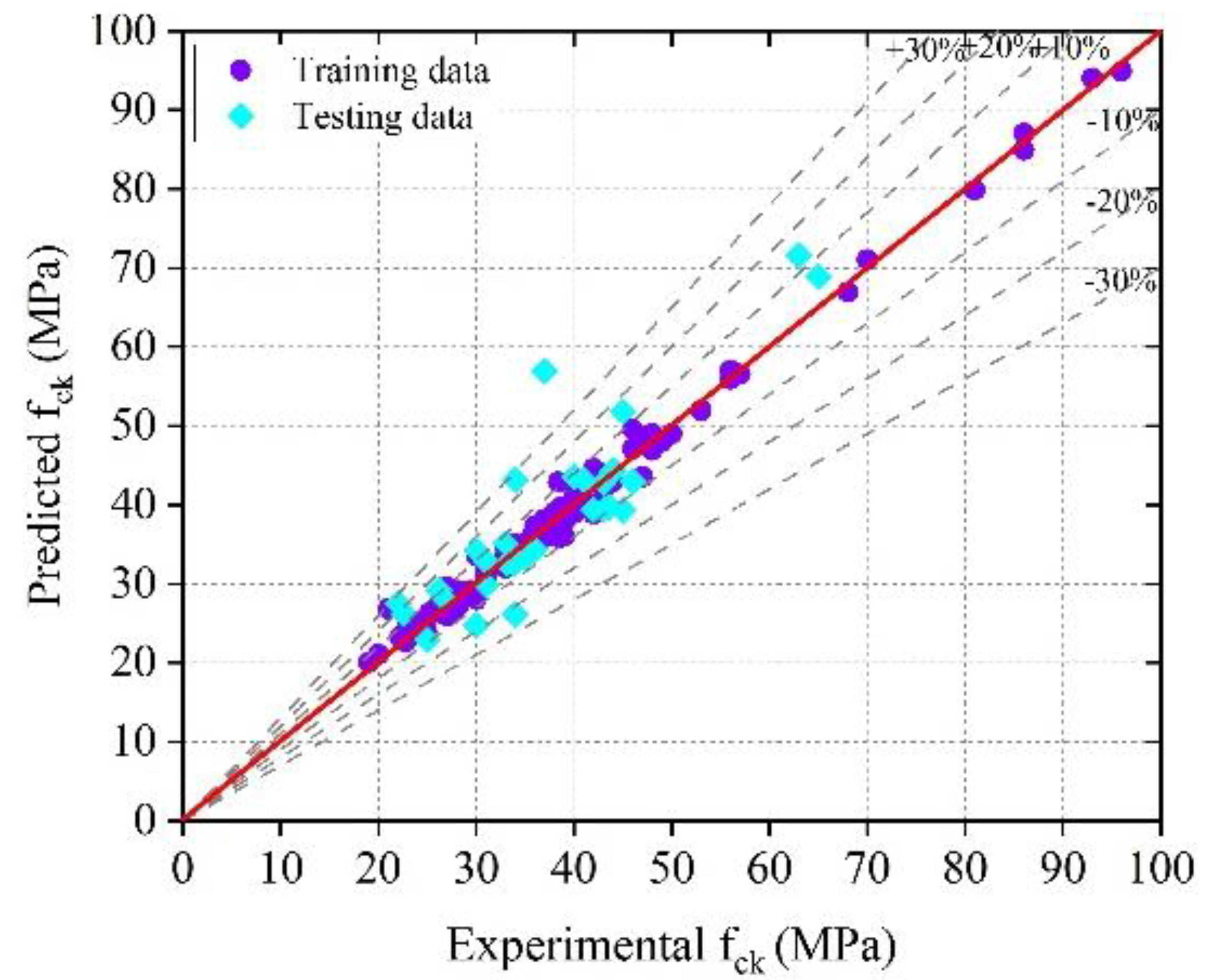
• The optimized GPR model had the greatest accuracy, with less variation in the experimental and predicted values in terms of errors.
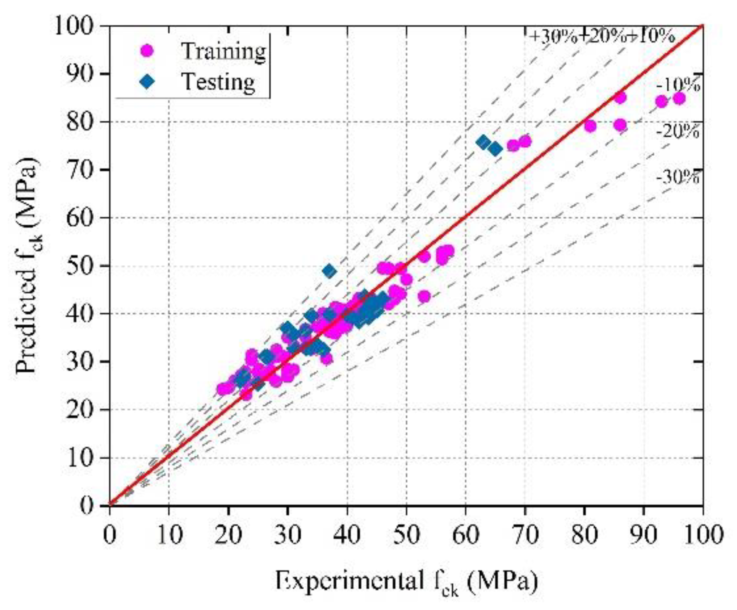
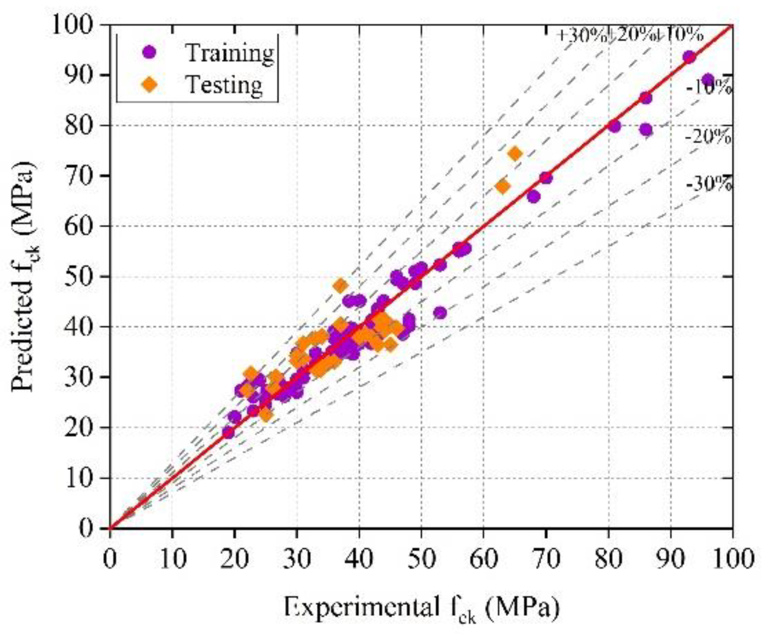
• The optimized GPR model provided training and testing correlation coefficients (R) of 0.9933 and 0.8915, respectively, and the optimized SVMR model provided training and testing correlation coefficients (R) of 0.9947 and 0.8882, respectively. The results indicate that the optimized GPR and SVMR models can predict the compressive strength with higher reliability and accuracy.
• The accuracy of the ML models decreased (based on the R, MAE, MAPE, and RMSE assessment criteria) in the following sequence: optimized GPR, optimal SVMR, GPR, SVMR, Optimized EL, and EL.

The machine learning models were excellent in capturing the intricate nonlinear correlations between the six input parameters and compressive strength. They may be used to quickly assess the compressive strength of LWC without the need to perform expensive and time-consuming experiments. More crucially, the machine learning-based estimation tools enable easy exploration of essential parameters, resulting in a cost-effective and trustworthy design. The machine learning approach is a strong instrument for engineering analysis. The proposed optimized GPR model can only perform effectively for data that fall within the range of the datasets used for creating the models, which is a limitation of this study. The accuracy of these models can be further enhanced using a metaheuristic algorithm and by adding more parameters in the database. In future work, the density of lightweight concrete can be predicted.

References

1. Aslani, F.; Ma, G.; Wan, D.L.Y.; Muselin, G. Development of high-performance self-compacting concrete using waste recycled concrete aggregates and rubber granules. J. Clean. Prod. 2018, 182, 553–566. [Google Scholar] [CrossRef]
2. Bicer, A.; Kar, F. The effects of apricot resin addition to the light weight concrete with expanded polystyrene. J. Adhes. Sci. Technol. 2017, 31, 2335–2348. [Google Scholar] [CrossRef]
3. Zeyad, A.M.; MJohari, A.M.; Tayeh, B.A.; Yusuf, M.O. Pozzolanic reactivity of ultrafine palm oil fuel ash waste on strength and durability performances of high strength concrete. J. Clean. Prod. 2017, 144, 511–522. [Google Scholar] [CrossRef]
4. Thienel, K.-C.; Haller, T.; Beuntner, N. Lightweight concrete—from basics to innovations. Materials 2020, 13, 1120. [Google Scholar] [CrossRef] [PubMed] [Green Version]
5. ACI Committee 213. ACI 213R-14 Guide for Structural Lightweight-Aggregate Concrete; American Concrete Institute: Farmington Hills, MI, USA, 2014. [Google Scholar]
6. Wongkeo, W.; Thongsanitgarn, P.; Pimraksa, K.; Chaipanich, A. Compressive strength, flexural strength and thermal conductivity of autoclaved concrete block made using bottom ash as cement replacement materials. Mater. Des. 2012, 35, 434–439. [Google Scholar] [CrossRef]
7. Chou, J.-S.; Pham, A.-D. Enhanced artificial intelligence for ensemble approach to predicting high performance concrete compressive strength. Constr. Build. Mater. 2013, 49, 554–563. [Google Scholar] [CrossRef]
8. Zhang, X.; Akber, M.Z.; Zheng, W. Prediction of seven-day compressive strength of field concrete. Constr. Build. Mater. 2021, 305, 124604. [Google Scholar] [CrossRef]
9. Asteris, P.G.; Skentou, A.D.; Bardhan, A.; Samui, P.; Pilakoutas, K. Predicting concrete compressive strength using hybrid ensembling of surrogate machine learning models. Cem. Concr. Res. 2021, 145, 106449. [Google Scholar] [CrossRef]
10. Alshihri, M.M.; Azmy, A.M.; El-Bisy, M.S. Neural networks for predicting compressive strength of structural light weight concrete. Constr. Build. Mater. 2009, 23, 2214–2219. [Google Scholar] [CrossRef]
11. Omran Behzad, A.; Chen, Q.; Jin, R. Comparison of data mining techniques for predicting compressive strength of environmentally friendly concrete. J. Comput. Civ. Eng. 2016, 30, 04016029. [Google Scholar] [CrossRef] [Green Version]
12. Yaseen, Z.M.; Deo, R.C.; Hilal, A.; Abd, A.M.; Bueno, L.C.; Salcedo-Sanz, S.; Nehdi, M.L. Predicting compressive strength of lightweight foamed concrete using extreme learning machine model. Adv. Eng. Softw. 2018, 115, 112–125. [Google Scholar] [CrossRef]
13. Kandiri, A.; Sartipi, F.; Kioumarsi, M. Predicting compressive strength of concrete containing recycled aggregate using modified ANN with different optimization algorithms. Appl. Sci. 2021, 11, 485. [Google Scholar] [CrossRef]
14. Tien Bui, D.; Abdullahi, M.A.; Ghareh, S.; Moayedi, H.; Nguyen, H. Fine-tuning of neural computing using whale optimization algorithm for predicting compressive strength of concrete. Eng. Comput. 2021, 37, 701–712. [Google Scholar] [CrossRef]
15. Sharafati, A.; Asadollah, S.B.H.S.; Al-Ansari, N. Application of bagging ensemble model for predicting compressive strength of hollow concrete masonry prism. Ain Shams Eng. J. 2021, 12, 3521–3530. [Google Scholar] [CrossRef]
16. Xu, J.; Zhou, L.; He, G.; Ji, X.; Dai, Y.; Dang, Y. Comprehensive machine learning-based model for predicting compressive strength of ready-mix concrete. Materials 2021, 14, 1068. [Google Scholar] [CrossRef]
17. ASTM C330M-17a. Standard Specification for Lightweight Aggregates for Structural Concrete; ASTM International: West Conshohocken, PA, USA, 2017. [Google Scholar]
18. Faust, T. Leichtbeton im Konstruktiven Ingenieurbau; Ernst & Sohn: Berlin, Germany, 2003; p. 307. ISBN 3-433-01613-5. [Google Scholar]
19. Sveindottir, E.L.; Maage, M.; Poot, S.; Hansen, E.A.; Bennenk, H.W.; Helland, S.; Norden, G.; Kwint, E.; Milencovic, A.; Smeplass, S.; et al. Light Weight Aggregates-Datasheets. Brite Euram Proj. Euro Lightcon. 1997, 132. [Google Scholar] [CrossRef]
20. Pauw, A. Structural lightweight aggregate concrete (concrete technology, structural design). In Proceedings of the 8th IABSE Congress, New York, NY, USA, 9–14 September 1968; pp. 541–557. [Google Scholar]
21. Siamardi, K. Optimization of fresh and hardened properties of structural light weight self-compacting concrete mix design using response surface methodology. Constr. Build. Mater. 2022, 317, 125928. [Google Scholar] [CrossRef]
22. Liu, X.; Du, H.; Zhang, M.-H. A model to estimate the durability performance of both normal and lightweight concrete. Constr. Build. Mater. 2015, 80, 255–261. [Google Scholar] [CrossRef] [Green Version]
23. Kim, Y.J.; Choi, Y.W.; Lachemi, M. Characteristics of self-consolidating concrete using two types of lightweight coarse aggregates. Constr. Build. Mater. 2010, 24, 11–16. [Google Scholar] [CrossRef]
24. Bogas, J.A.; Gomes, A. A simple mix design method for structural lightweight aggregate concrete. Mater. Struct. 2013, 46, 1919–1932. [Google Scholar] [CrossRef]
25. Bogas, J.A.; de Brito, J.; Figueiredo, J.M. Mechanical characterization of concrete produced with recycled lightweight expanded clay aggregate concrete. J. Clean. Prod. 2015, 89, 187–195. [Google Scholar] [CrossRef]
26. Nguyen, L.H.; Beaucour, A.L.; Ortola, S.; Noumowé, A. Influence of the volume fraction and the nature of fine lightweight aggregates on the thermal and mechanical properties of structural concrete. Constr. Build. Mater. 2014, 51, 121–132. [Google Scholar] [CrossRef]
27. Choi, Y.W.; Kim, Y.J.; Shin, H.C.; Moon, H.Y. An experimental research on the fluidity and mechanical properties of high-strength lightweight self-compacting concrete. Cem. Concr. Res. 2006, 36, 1595–1602. [Google Scholar] [CrossRef]
28. Yang, C.-C.; Huang, R. Approximate strength of lightweight aggregate using micromechanics method. Adv. Cem. Based Mater. 1998, 7, 133–138. [Google Scholar] [CrossRef]
29. Kockal, N.U.; Ozturan, T. Strength and elastic properties of structural lightweight concretes. Mater. Des. 2011, 32, 2396–2403. [Google Scholar] [CrossRef]
30. Gesoğlu, M.; Özturan, T.; Güneyisi, E. Effects of fly ash properties on characteristics of cold-bonded fly ash lightweight aggregates. Constr. Build. Mater. 2007, 21, 1869–1878. [Google Scholar] [CrossRef]
31. Chi, J.M.; Huang, R.; Yang, C.C.; Chang, J.J. Effect of aggregate properties on the strength and stiffness of lightweight concrete. Cem. Concr. Compos. 2003, 25, 197–205. [Google Scholar] [CrossRef]
32. Kayali, O. Fly ash lightweight aggregates in high performance concrete. Constr. Build. Mater. 2008, 22, 2393–2399. [Google Scholar] [CrossRef]
33. Güneyisi, E.; Gesoğlu, M.; Booya, E. Fresh properties of self-compacting cold bonded fly ash lightweight aggregate concrete with different mineral admixtures. Mater. Struct. 2012, 45, 1849–1859. [Google Scholar] [CrossRef]
34. Rossignolo, J.A.; Agnesini, M.V.C.; Morais, J.A. Properties of high-performance LWAC for precast structures with brazilian lightweight aggregates. Cem. Concr. Compos. 2003, 25, 77–82. [Google Scholar] [CrossRef]
35. Aslam, M.; Shafigh, P.; Jumaat, M.Z.; Lachemi, M. Benefits of using blended waste coarse lightweight aggregates in structural lightweight aggregate concrete. J. Clean. Prod. 2016, 119, 108–117. [Google Scholar] [CrossRef]
36. Alengaram, U.J.; Mahmud, H.; Jumaat, M.Z. Enhancement and prediction of modulus of elasticity of palm kernel shell concrete. Mater. Des. 2011, 32, 2143–2148. [Google Scholar] [CrossRef]
37. Wee, T.H.; Chin, M.S.; Mansur, M.A. Stress-strain relationship of high-strength concrete in compression. J. Mater. Civ. Eng. 1996, 8, 70–76. [Google Scholar] [CrossRef]
38. Del Rey Castillo, E.; Almesfer, N.; Saggi, O.; Ingham, J.M. Lightweight concrete with artificial aggregate manufactured from plastic waste. Constr. Build. Mater. 2020, 265, 120199. [Google Scholar] [CrossRef]
39. Ofuyatan, O.M.; Olutoge, F.; Omole, D.; Babafemi, A. Influence of palm ash on properties of light weight self-compacting concrete. Clean. Eng. Technol. 2021, 4, 100233. [Google Scholar] [CrossRef]
40. Wongkvanklom, A.; Posi, P.; Khotsopha, B.; Ketmala, C.; Pluemsud, N.; Lertnimoolchai, S.; Chindaprasirt, P. Structural lightweight concrete containing recycled lightweight concrete aggregate. KSCE J. Civ. Eng. 2018, 22, 3077–3084. [Google Scholar] [CrossRef]
41. Kumar, A.; Arora, H.C.; Mohammed, M.A.; Kumar, K.; Nedoma, J. An optimized neuro-bee algorithm approach to predict the FRP-concrete bond strength of RC beams. IEEE Access 2022, 10, 3790–3806. [Google Scholar] [CrossRef]
42. Kumar, A.; Arora, H.C.; Kumar, K.; Mohammed, M.A.; Majumdar, A.; Khamaksorn, A.; Thinnukool, O. Prediction of FRCM-concrete bond strength with machine learning approach. Sustainability 2022, 14, 845. [Google Scholar] [CrossRef]
43. Armaghani, D.J.; Asteris, P.G.; Fatemi, S.A.; Hasanipanah, M.; Tarinejad, R.; Rashid, A.S.A.; Huynh, V.V. On the use of neuro-swarm system to forecast the pile settlement. Appl. Sci. 2020, 10, 1904. [Google Scholar] [CrossRef] [Green Version]
44. Pei, Z.; Wei, Y. Prediction of the bond strength of FRP-to-concrete under direct tension by ACO-based ANFIS approach. Compos. Struct. 2022, 282, 115070. [Google Scholar] [CrossRef]
45. Kopsiaftis, G.; Protopapadakis, E.; Voulodimos, A.; Doulamis, N.; Mantoglou, A. Gaussian process regression tuned by bayesian optimization for seawater intrusion prediction. Comput. Intell. Neurosci. 2019, 2019, 2859429. [Google Scholar] [CrossRef] [PubMed]
46. Vapnik, V. The Nature of Statistical Learning Theory; Springer Science & Business Media: Berlin/Heidelberg, Germany, 1999. [Google Scholar]
47. Olayiwola, T.; Ogolo, O.; Yusuf, F. Modeling the acentric factor of binary and ternary mixtures of ionic liquids using advanced intelligent systems. Fluid Phase Equilibria 2020, 516, 112587. [Google Scholar] [CrossRef]
48. Liu, Z.; Guo, A. Empirical-based support vector machine method for seismic assessment and simulation of reinforced concrete columns using historical cyclic tests. Eng. Struct. 2021, 237, 112141. [Google Scholar] [CrossRef]
49. Kumar, K.; Saini, R.P. Development of correlation to predict the efficiency of a hydro machine under different operating conditions. Sustain. Energy Technol. Assess. 2022, 50, 101859. [Google Scholar] [CrossRef]
50. Chen, S.-Z.; Zhang, S.-Y.; Han, W.-S.; Wu, G. Ensemble learning based approach for frp-concrete bond strength prediction. Constr. Build. Mater. 2021, 302, 124230. [Google Scholar] [CrossRef]
51. Yang, Y. Chapter 4—ensemble learning. In Temporal Data Mining via Unsupervised Ensemble Learning; Yang, Y., Ed.; Elsevier: Amsterdam, The Netherlands, 2017; pp. 35–56. [Google Scholar] [CrossRef]
52. Wang, Z.; Wang, Y.; Zeng, R.; Srinivasan, R.S.; Ahrentzen, S. Random forest based hourly building energy prediction. Energy Build. 2018, 171, 11–25. [Google Scholar] [CrossRef]
Figure 1. Different types of concrete.
Sustainability 14 02404 g001
Figure 2. Types of LWA.
Sustainability 14 02404 g002
Figure 3. Requirements for LWA as per ASTM C331M.
Sustainability 14 02404 g003
Figure 4. Scatterplot matrix of the compressive strength of the LWC database with correlation. C, W, FA, LWCA, NWCA, w/c, and fck.
Sustainability 14 02404 g004
Figure 5. Distribution pattern of: (a) cement content, (b) water content, (c) fine aggregate, (d) normal weight coarse aggregate, (e) lightweight coarse aggregate, (f) water-cement ratio, (g) compressive strength of concrete.
Sustainability 14 02404 g005
Figure 6. Sketch map of the SVM model.
Sustainability 14 02404 g006
Figure 7. The framework of 10-fold cross-validation to develop machine learning models to predict the compressive strength of LWC.
Sustainability 14 02404 g007
Figure 8. Illustration of regression plot between the experimental and predicted values of the compressive strength of LWC—GPR.
Sustainability 14 02404 g008
Figure 9. Optimized GPR model (normalized values).
Sustainability 14 02404 g009
Figure 10. Illustration of regression plot between the experimental and predicted values of the compressive strength of LWC—Optimized GPR.
Sustainability 14 02404 g010
Figure 11. Illustration of regression plot between the experimental and predicted values of the compressive strength of LWC—SVMR.
Sustainability 14 02404 g011
Figure 12. Optimized SVMR model (normalized values).
Sustainability 14 02404 g012
Figure 13. Illustration of regression plot between the experimental and predicted values of the compressive strength of LWC—Optimized SVMR.
Sustainability 14 02404 g013
Figure 14. Illustration of regression plot between the experimental and predicted values of the compressive strength of LWC—EL.
Sustainability 14 02404 g014
Figure 15. Optimized EL model (normalized values).
Sustainability 14 02404 g015
Figure 16. Illustration of regression plot between the experimental and predicted values of the compressive strength of LWC—Optimized EL.
Sustainability 14 02404 g016
Figure 17. Predicted errors performed by: (a) GPR (b) SVMR (c) EL, (d) Optimized GPR (e) Optimized SVM, and (f) Optimized EL.table
Sustainability 14 02404 g017