Joint Estimation of Adsorptive Contaminant Source and Hydraulic Conductivity Using an Iterative Local Updating Ensemble Smoother with Geometric Inflation Selection

Abstract

The joint estimation of groundwater contaminant source characteristics and hydraulic conductivity is of great significance for reactive contaminant transport models in heterogeneous subsurface media. The accurate determination of the sorption parameters of such contaminants is also a key prerequisite for estimating the parameters of the groundwater system. In this study, to investigate the impact of the sorption parameter field on the accuracy of hydraulic conductivity and source characteristics estimation, numerical experiments were conducted in a synthetic aquifer considering the contaminant sorption process in groundwater models with varying sorption parameter settings. Iterative local updating ensemble smoother with geometric inflation selection (ILUES-GEO) was employed to assimilate hydraulic head and contaminant concentration data to jointly estimate the contaminant source information and hydraulic conductivity in a heterogeneous aquifer. The results indicated that the ILUES-GEO successfully recovers contaminant source information simultaneously with hydraulic conductivity, and its performance improves as more accurate sorption parameters are introduced. Furthermore, the influence of the ILUES algorithm parameters and ensemble size is investigated to improve the estimation accuracy. Additionally, the characterization of contaminant sources and hydraulic conductivity fields is influenced by the number and locations of measurements. This study can help to understand the significance of sorption parameter setting for the joint estimation of reactive contaminant source and hydraulic parameters.

1. Introduction

Contaminant transport, being a vital process, influences the sustainable utilization and quality of water in the subsurface system. Hazardous substances could be carried by contaminated groundwater, posing a threat to both the ecosystem and human health. The variability of the groundwater contaminant concentration mainly depends on diffusion, sorption, and potential geobiochemical processes (e.g., biodegradation), among which the sorption term is introduced to maintain the solute in the immobile zone and slow down its travel time through the porous media [1,2,3]. Many researchers have addressed the heterogeneous rates of mass transfer in transport models as a result of the local variability in the diffusion and sorption properties of the porous medium [4,5]. Haggerty et al. have further demonstrated that mass-transfer timescales can be varied due to the varying sorption rates [6]. Determining effective sorption parameters is crucial for estimating other system parameters and describing subsurface heterogeneity [7].

Due to the large number of inadequately understood subsurface characteristics (e.g. hydraulic conductivity) and model uncertainties, numerical models for predicting the flow and solute transport in groundwater have limited accuracy [8,9]. Recently, advanced techniques have made available many types of observation data that are indirectly related to models, necessitating the development of new methods to reconcile information from multiple sources dynamically [10,11,12]. To improve the predictive capacity of these models, efforts have been focused on calibrating the model parameter distributions using inverse methodologies and diverse measurement data [13,14,15,16]. Data assimilation, also known as a stochastic inverse method, whose advantage is that its scheme constitutes model errors from uncertain model parameters, model structures, and inputs (initial conditions), has been widely used in hydrogeology [17,18,19,20].

Ensemble-based data assimilation methods are popular because of their Monte Carlo nature; they are derivative free and well adapted to parallelization [21]. The Ensemble Kalman Filter (EnKF) proposed by Evensen [22] as an ensemble-based data assimilation method can update model parameters and state variables by sequentially assimilating available measurements and has gained popularity in multidisciplinary fields such as meteorology and hydrology [23,24,25,26,27]. Ensemble Smoother (ES) [28], in contrast to EnKF, assimilates the entire available data simultaneously to compute an updated model state estimate and avoids inconsistency issues between model parameters and state variables by transforming the parameter-state-estimation problem to a parameter-estimation problem [17,29,30]. Additionally, ES has a lower computational cost than EnKF since the ES update routine is performed only once with all available data and can be used independently of the simulation model, i.e., without recurring simulation models [19,31]. It has also been discussed that ES provides similar estimates as EnKF for solving the history-matching problem in reservoir simulation models more efficiently [32]. The ES and its variants have been successfully implemented in groundwater work [29,31,33]. Varied iterative forms of ES, in which the same data might be continuously assimilated to update the parameters or states, have also been proposed to improve the performance of ES in addressing substantially nonlinear situations. For instance, Ju et al. coupled an iterative ensemble smoother with a Gaussian process surrogate model to estimate the heterogeneous conductivity field in subsurface flow problems [17]. Li et al. developed an iterative normal-score ensemble smoother (NS-ES) to deal with the characterization of non-multi-Gaussian conductivities [29]. It is of interest to note that the iterative ES outperforms the original ES and EnKF in terms of computational efficiency and accuracy [34,35].

To improve the applicability and efficiency of ES for highly nonlinear problems, Zhang et al. proposed an iterative local updating ensemble smoother (ILUES), in which the local ensemble of each sample is defined by measuring the distance between this sample and the observations, and each sample is updated locally using the scheme of ES instead of globally updated [19]. In addition, to reduce the impact of non-linearity on the data match quality, the iterative scheme of ES is used to assimilate the same set of observation data multiple times to update the parameters. Mo et al. have constructed a deep autoregressive neural network surrogate model and implemented the ILUES algorithm as the inverse method to solve high-dimensional groundwater inverse problems with accurate identification results [36]. Emerick and Reynolds demonstrated that selecting the inflation factors in a decreasing order can improve the results of ES-MDA [34]. Additionally, Emerick proposed a novel procedure to select inflation factors in a geometrically decreasing sequence, which achieves desirable results for reservoir history-matching problems [37]. The contaminant source information and hydraulic conductivity field could not be obtained as straightforwardly and cost-efficiently as the concentration and head data. Moreover, the complete representation of these model parameters enables the characterization of important chemical and hydrologic processes. Therefore, it is particularly important to represent these parameters by solving the inversion problem. The computational cost of the ensemble-based data assimilation method to invert these parameters is fairly low compared to traditional simulation-optimization methods, which require the repeated calculation of the objective function. In this study, the geometric inflation factor selection method is integrated into ILUES, which is then employed using the inversion method to estimate the contaminant source characteristics and hydraulic parameters, taking into account the impact of sorption parameter determination.

The effect of the sorption parameter field on contaminant source and parameter estimation has, to the best of our knowledge, received little attention, despite the fact that several research studies have focused on mass transfer rates influenced by variability in sorption properties [38,39,40]. Moreover, the influence of the variability of the distribution coefficient is generally ignored in the parameter of inversion problem when the adsorptive contaminant is considered in the simulation model. In this study, we investigate the effect of determining the distribution coefficient field on the estimate of contaminant source and system parameters and test the efficiency of the proposed ILUES-GEO algorithm as the inverse approach. It is performed in a synthetic heterogeneous aquifer and investigated for three scenarios utilizing various Kd field determination methods. This work focuses on the performance of joint parameter inversion and the determination of the distribution coefficient for the entire study area, which is an important aspect of parameter estimation in cases where sorption is the main process of groundwater contaminant transport. The algorithm employed in this study is based on the method of [19], which has been shown as efficient in the parameter estimation case. However, for this study, firstly, the linear sorption process is addressed in the transport model and primarily concerned with the contribution of the accurate knowledge of the sorption parameters to the understanding of solute transport behavior and the estimation of contaminant source and system parameters. Secondly, the geometric inflation factor selection method is extended to the ILUES framework, which is used as the inversion method. Finally, the effects of the ensemble size and algorithm parameters of ILUES-GEO are systematically investigated to obtain the optimal parameter set for this study. In addition, we explore the influence of observation locations and the quantity of observations on the performance of ILUES-GEO in identifying groundwater sources and estimating parameters. The results are expected to serve as a reference for the application of the ILUES method to similar hydrogeological data assimilation problems.

The remainder of this work is organized as follows. Section 2 presents the detailed description of the ILUES-GEO algorithm and the basic theories of groundwater flow and transport with sorption processes. Section 3 outlines the framework of data assimilation and the three scenarios with different determination methods of sorption parameter field based on a synthetic example. In Section 4, the results obtained from assimilation experiments are discussed. Several conclusions are given in Section 5.

2. Methodology

2.1. Groundwater Flow and Transport Simulation

The governing partial differential equation for the steady-state saturated flow in a two-dimensional aquifer is generally described by:

$$\frac{\partial }{\partial x_i}\left(K_{ij}\frac{\partial h}{\partial x_j}\right)+W=0 i,j=1,2$$

(1)

where K_ij is the hydraulic conductivity [LT⁻¹], h is the hydraulic head [L], W is the volumetric source (positive) or sink (negative) flux per unit volume [T⁻¹], and x_i and x_j are the Cartesian coordinates. The head distribution can be used to determine the average linear velocity of groundwater flow v_i [LT⁻¹] according to Darcy’s law:

$${\upsilon }_i=-\frac{K_{ij}}{\theta }\frac{\partial h}{\partial x_i} i,j=1,2$$

(2)

The two-dimensional contaminant transport, including advection, dispersion, and adsorption processes in groundwater, is represented by the following equation:

$$R_d\frac{\partial \left(\theta C\right)}{\partial t}+\frac{\partial }{\partial x_i}\left(\theta {\upsilon }_{i}C\right)-\frac{\partial }{\partial x_i}\left(D_{ij}\theta \frac{\partial C}{\partial x_j}\right)-C_{S}W=0 i,j=1,2$$

(3)

where $\theta$ is the porosity, dimensionless, C is the contaminant concentration [ML⁻³], D_ij is the hydrodynamic dispersion coefficient (a second-order tensor) [L²T⁻¹], $C_S$ is the concentration of sources or sinks [ML⁻³], and R_d is the retardation factor.

Since the molecular diffusion is often much lower than the hydrodynamic dispersion, it is ignored in this study. The hydrodynamic dispersion coefficient D_ij [L²T⁻¹] can be defined as:

$$\left\{\begin{array}{l}{D}_{x_1{x}_1}=\left({\alpha }_L{v}_{x_1}^2+{\alpha }_T{v}_{x_2}^2\right)/\left|v\right|\\ D_{x_2{x}_2}=\left({\alpha }_L{v}_{x_2}^2+{\alpha }_T{v}_{x_1}^2\right)/\left|v\right|\\ D_{x_1{x}_2}=D_{x_2{x}_1}=\left({\alpha }_L-{\alpha }_T\right)v_{x_1}{v}_{x_2}/\left|v\right|\end{array}\right.$$

(4)

where, ${\alpha }_L$ is the longitudinal dispersivity, ${\alpha }_T$ is the transverse dispersivity [L], and |v| is the magnitude of velocity vector.

A linear isotherm is common in groundwater contamination where the adsorbed concentration is relatively low compared to the adsorptive capacity of the soil, i.e., adsorption conditions far below saturation [41]. Thus, the linear sorption isotherm is assumed in the numerical experiments of this study, and the retardation factor, R_d, is expressed as follows:

$$R_d=1+\frac{{\rho }_b{K}_d}{\theta }$$

(5)

where $K_d$ is the sorption distribution coefficient [L³M⁻¹] representing the ratio of sorbed and dissolved concentrations at equilibrium, ${\rho }_b$ is the bulk density of the immobile area of porous media [ML⁻³], and $\theta$ is the porosity of porous media as previously mentioned.

Both contaminant source characteristics and system parameters, including source location, source strengths, and heterogeneous aquifer conductivity field, are identified in this groundwater contamination inverse problem. In addition, adsorption is considered in this inverse problem, and the distribution coefficient field plays a significant part in the solute transport simulation. The proposed identification problem is processed by handling both hydraulic head and solute concentration data. Considered is a time-varying source strength, with the strength of each time segment represented by the parameter, $S_{si},i=1,\cdots ,n$, where n is the number of time segments. Both the distribution coefficient field (K_d) and the hydraulic conductivity field (K) are regarded as random fields. This study attempts, on the one hand, to simultaneously determine the contaminant source characteristics (i.e., source location and source strength) and the hydraulic conductivity field. When adsorption is addressed in the solute transport process, the distribution coefficient field also serves as a heterogeneous field due to the heterogeneity of the aquifer. The accuracy of joint estimations of source characteristics and hydraulic conductivity field may be influenced by the determination of a reasonable distribution coefficient field.

2.2. Data Assimilation Method

It is assumed that the relation between the vector of measurements and the vector of model parameters can be simplified in the form:

$$d=G\left(m\right)+\epsilon ,$$

(6)

$d$ is the measurement vector, $m$ is the vector of model parameters, $G\left(•\right)$ is the forward model, and $\epsilon$ is a vector of Gaussian-distributed measurement error with mean $E\left(\epsilon \right)=0$ and covariance $C_D=E\left[{\epsilon }_j {\epsilon }_j^T\right]$.

2.2.1. Ensemble Smoother

The basic ES analysis equation can be written as:

$$m_j^a=m_j^f+C_{MD}^f{(C_{DD}^f+C_D)}^{-1}\left[d_j-G\left(m_j^f\right)\right],$$

(7)

$C_{MD}^f$ is the cross-variance matrix between the prior vector of model parameter $m^f$ and the measurement vector $d^f$; $C_{DD}^f$ is the $N_d\times N_d$ auto-covariance matrix of measurement $D^f$; $N_d$ is the total number of measurements assimilated; $d_j~N\left(d_{obs},C_D\right)$ is the measurement with $d_{obs}$ representing the $N_d\times 1$ vector of observation data and $C_D=E\left[{\epsilon }_j {\epsilon }_j^T\right]$.

For $j=1,2,\cdots ,N_e$, where $N_e$ denotes the size of ensemble members.

2.2.2. Iterative Local Updating Ensemble Smoother with Geometric Inflation Selection

The details of ILUES-GEO can be implemented in the following steps [19]:

Step1: Initialization. $N_e$ equally likely stochastic parameter realizations from prior distribution are generated as the initial parameter ensemble. The output ensemble for the initial parameter ensemble could also be generated by solving the forward model.

$$M^{ini}=\left[m_1^{ini},m_2^{ini},\cdots ,m_{N_e}^{ini}\right]$$

(8)

$$D^{ini}=\left[G\left(m_1^{ini}\right),G\left(m_2^{ini}\right),\cdots ,G\left(m_{N_e}^{ini}\right)\right]$$

(9)

The subscript represents the index of the ensemble member, and the superscript “ini” is short for “initialization”, which means the initial iteration.

Step2: Determination of local ensemble.

To determine the local ensemble of the sample $m_j^f\left(j=1,2,\cdots ,N_e\right)$, the distance $J\left(m\right)$ between the measurements $d$ and the sample $m_j^f$ is measured synthetically from both the space of the model responses $J_1$ and the model parameters $J_2$:

$$J\left(m\right)=J_1\left(m\right)/J_1^{max}+\beta ·J_2\left(m\right)/J_2^{max}$$

(10)

$$J_1\left(m\right)={\left[G\left(m\right)-d\right]}^T{C}_D^{-1}\left[G\left(m\right)-d\right],$$

(11)

$$J_2\left(m\right)={\left[m-m_j^f\right]}^T{C}_{MM}^{-1}\left[m-m_j^f\right],$$

(12)

$J_1\left(m\right)$ is the distance between the predicted data by forward model $G\left(m\right)$ and the measurements $d$; $J_2\left(m\right)$ is the distance between the model parameters $m$ and the selected samples $m_j^f$; $\beta \in \left(0,\infty \right)$ represents the relative weight of two distance metrics, where $J_1^{max}$ and $J_2^{max}$ are the maximum values of $J_1\left(m\right)$ and $J_2\left(m\right)$, respectively. $C_{MM}$ is the auto-covariance matrix of the model parameters $m$.

Step3: Update the local ensemble.

The local ensemble of $m_j^f$, containing the $N_{loc}=\alpha N_e\left(\alpha \in \left(0,1\right]\right)$ samples with $N_{loc}$ lowest $J$ values, can be updated by ensemble smoother:

$$m_{j,k}^a=m_{j,k}^f+C_{MD}^{loc,f}{(C_{DD}^{loc,f}+{\mu }_i{C}_D)}^{-1}\left[d_k-G\left(m_{j,k}^f\right)\right],$$

(13)

where $k=1,\cdots ,N_{loc}$; $\alpha$ is the ratio between the local ensemble $M_j^{loc,f}$ and the global ensemble $M^f$; $C_{DD}^{loc,f}$ is the $N_d\times N_d$ auto-covariance matrix of measurement $D^{loc,f}$; $N_d$ is the total number of measurements assimilated; $d_k\sim {\rm N}\left(d_{obs},C_D\right)$ is the measurement with $d_{obs}$ representing the $N_d\times 1$ vector of observation data and $C_D=E\left[{\epsilon }_k {\epsilon }_k^T\right]$ representing the $N_d\times N_d$ covariance matrix of measurement errors of observation data. ${\mu }_i>1$ represents data-error covariance inflation factor and is selected based on the following condition:

$${\displaystyle \sum }_{i=1}^{I_{MAX}}\frac{1}{{\mu }_i}=1$$

(14)

where $I_{MAX}$ is the pre-defined number of iterations.

An inflation factor selection method is adopted in the ILUES framework, which is proposed by [37]. The final inflation factor ${\mu }_{I_{MAX}}$ is specified first, and the previous inflation factors are computed geometrically in ascending order by solving the following formula:

$${\mu }_i={\gamma }^{i-I_{MAX}}{\mu }_{I_{MAX}} , i=1,\dots ,I_{MAX}$$

(15)

The coefficient $\gamma \in \left(0,1\right]$ can be calculated by solving $f_2\left(\gamma \right)=0$ using the bisection method, defined as follows:

$$f_2\left(\gamma \right)=\frac{1-{\gamma }^{I_{MAX}}}{1-\gamma }-{\mu }_{I_{MAX}}$$

(16)

Randomly selected from the updated local ensemble $M_j^{loc,a}=\left[m_{j,1}^a,m_{j,2}^a,\cdots ,m_{j,N_{loc}}^a\right]$, sample $m_j^{loc,a}$ is regarded as the updated sample of $m_j^f\left(j=1,2,\cdots ,N_e\right)$. Following this procedure, the updated global ensemble $M^a=\left[m_1^{loc,a},m_2^{loc,a},\cdots ,m_{N_e}^{loc,a}\right]$ can be obtained.

The framework of the ILUES-GEO algorithm is shown in Figure 1.

3. Illustrative Example

3.1. Problem Description

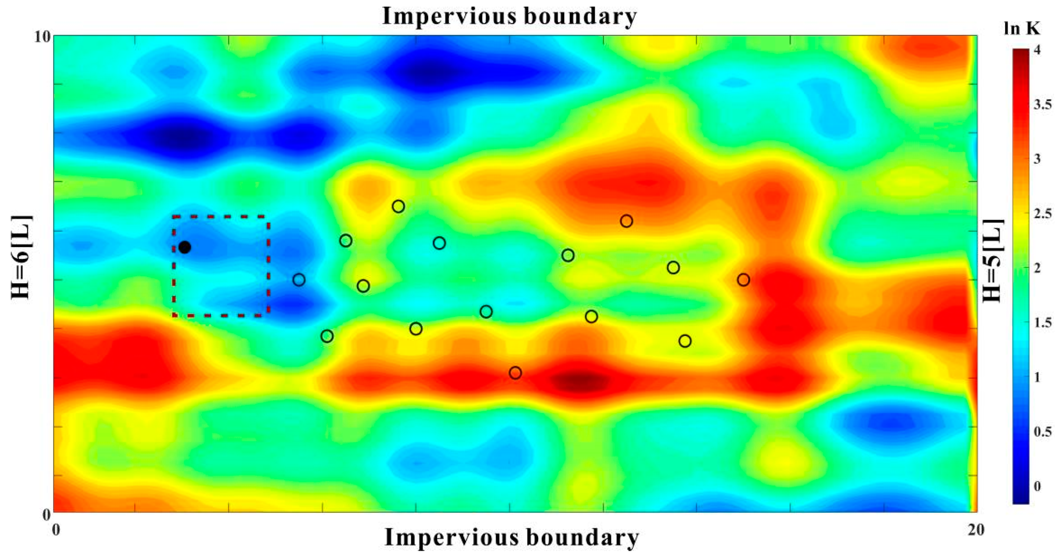
A two-dimensional, steady groundwater flow through an anisotropic, heterogeneous, saturated aquifer revised after that of [19] is utilized in the illustrative case to test the applicability of the ILUES algorithm to estimate the hydraulic conductivity field and characterize the groundwater contaminant source simultaneously considering the heterogeneous distribution coefficient field by assimilating both head and solute concentration measurements. The hypothetical aquifer extends over a domain of 20 × 10 [L] and is discretized in two dimensions into 80 columns by 40 rows (i.e., 0.25 × 0.25 [L] square grid cells) (Figure 2). No flow conditions are prescribed on the upper and lower boundaries. The prescribed constant heads on the western and eastern boundaries are equal to 6 and 5 [L], respectively. The related model parameters are listed in

Table 1. Primary parameters used in solving the steady state flow equation and the contaminant transport equation.

Parameters	Unit	Value
Row	Dimensionless	40
Column	Dimensionless	80
Grid spacing in x direction	[L]	0.25
Grid spacing in y direction	[L]	0.25
Saturated thickness	[L]	10
Effective porosity	Dimensionless	0.35
Longitudinal dispersivity	[L]	0.3
Transverse dispersivity	[L]	0.03

.

A contaminant source with a time-varying strength at an unknown location releasing from 0 [T] to 6 [T] is considered in this study, with the mass-loading rate denoting the source strength. The contaminant source is identified by eight parameters, which include two source location coordinates $(S_x,S_y)$ and the time-varying strength in six time intervals, i.e., $S_{si}$ [MT⁻¹] during $\left[t_{i-1},t_i\right]$, where $t_i=i\left[T\right],i=1,\cdots , 6$. The prior distribution of the eight parameters is uniform, as depicted in

Table 2. The reference values and prior distributions of the contaminant source parameters for the case study.

Parameter	$$\begin{gathered} {\mathit{S}}_{\mathit{x}} \\ \left[\mathbf{L}\right] \end{gathered}$$	$$\begin{gathered} {\mathit{S}}_{\mathit{y}} \\ \left[\mathbf{L}\right] \end{gathered}$$	$$\begin{gathered} {\mathit{S}}_{\mathit{s}1} \\ \left[{\mathbf{MT}}^{-1}\right] \end{gathered}$$	$$\begin{gathered} {\mathit{S}}_{\mathit{s}2} \\ \left[{\mathbf{MT}}^{-1}\right] \end{gathered}$$	$$\begin{gathered} {\mathit{S}}_{\mathit{s}3} \\ \left[{\mathbf{MT}}^{-1}\right] \end{gathered}$$	$$\begin{gathered} {\mathit{S}}_{\mathit{s}4} \\ \left[{\mathbf{MT}}^{-1}\right] \end{gathered}$$	$$\begin{gathered} {\mathit{S}}_{\mathit{s}5} \\ \left[{\mathbf{MT}}^{-1}\right] \end{gathered}$$	$$\begin{gathered} {\mathit{S}}_{\mathit{s}6} \\ \left[{\mathbf{MT}}^{-1}\right] \end{gathered}$$
Prior	$\mathcal{U}\left[3,5\right]$	$\mathcal{U}\left[4,6\right]$	$\mathcal{U}\left[0,8\right]$	$\mathcal{U}\left[0,8\right]$	$\mathcal{U}\left[0,8\right]$	$\mathcal{U}\left[0,8\right]$	$\mathcal{U}\left[0,8\right]$	$\mathcal{U}\left[0,8\right]$
True value	3.1755	5.4240	5.0148	2.7255	5.7100	7.6553	4.6193	5.5584

. Note that under the assumption of given prior distributions, the true values of the contaminant source parameters are generated randomly.

Considering the spatial heterogeneity, the reference conductivity and distribution coefficient fields are assumed to be log-Gaussian random fields,

$$Y\left(l\right)=exp\left(F\left(l\right)\right),F\left(l\right)~N\left(m\left(l\right),C\left(·,·\right)\right),Y=K_d,K$$

(17)

The following expressions are used to describe the spatial correlation structure of the log-conductivity and log-distribution coefficient fields:

$${\gamma }_F={\sigma }_F^2\exp (-\sqrt{{\left(\frac{l_x-l_x^{\prime }}{{\lambda }_x}\right)}^2+{\left(\frac{l_y-l_y^{\prime }}{{\lambda }_y}\right)}^2})$$

(18)

where ${\sigma }_F^2$ is the variance, $l=\left(l_x,l_y\right)$ and $l^{\prime }=\left(l_x^{\prime },l_y^{\prime }\right)$ denote two arbitrary spatial locations, and ${\lambda }_x$ and ${\lambda }_y$ are the correlation lengths along the x and y directions, respectively. This study takes into account heterogeneous hydraulic conductivity and distribution coefficient fields with a length scale of $\frac{{\lambda }_x}{L_x}=\frac{{\lambda }_y}{L_y}=0.25$, where $L_{x }$ and $L_y$ are the domain sizes along both directions. The variogram components of each random function are listed in

Table 3. Random function parameters for modeling the spatial distribution of log-conductivity and log-distribution coefficients.

	Variogram Type	Mean	Standard Deviation	λx[L]	λy[L]
lnK(ln[L/T])	Gaussian	2	1	5	2.5
lnKd(ln[L3/M])	Gaussian	1.9461	0.5	5	2.5

.

An inverse problem with high-dimensional inputs may result in a heavy computational burden due to the repeated execution of forward models to obtain satisfactory results. Thus, to improve the computational efficiency of ILUES-GEO, the log-conductivity and log-distribution coefficient fields are parameterized by truncating a Karhunen–Loève expansion (KLE) [42]. Let $\mathit{ln}Y\left(x,\omega \right)$ be a random event, where $Y=K_d,K$, x represents the position vector defined over the domain D, and $\omega$ belongs to a probability space $\Omega$ of a random process. $\langle \mathit{ln}Y\left(x,\omega \right)\rangle$ denotes the mean component of $\mathit{ln}Y\left(x,\omega \right)$ over all possible realizations of the process. A covariance function $C\left(x,y\right)$ that is bounded, symmetric, and positive definite must be defined to construct the KLE, and it can be decomposed into:

$$C\left(x,y\right)={\displaystyle \sum }_{i=1}^{\infty }{\tau }_i{f}_i\left(x\right)f_i\left(y\right)$$

(19)

where ${\tau }_i$ and $f_i\left(x\right)$ are eigenvalues and eigenfunctions of the correlation function, respectively, and can be solved according to the second kind of the homogeneous Fredholm integral equation

$${{\displaystyle \int }}_{D}C\left(x,y\right)f_i\left(x\right)dx={\tau }_i{f}_i\left(y\right)$$

(20)

The eigenfunctions $f_i\left(x\right)$ are deterministic and orthogonal functions and form a complete set. The normalization criterion of the eigenfunctions $f_i\left(x\right)$ can be written as:

$${{\displaystyle \int }}_D{f}_i\left(x\right)f_j\left(x\right)dx={\delta }_{ij},i,j\ge 1$$

(21)

The expansion of the random process $\mathit{ln}Y\left(x,\omega \right)$, is as follows:

$$\mathit{ln}Y\left(x,\omega \right)=\langle \mathit{ln}Y\left(x,\omega \right)\rangle +{\displaystyle \sum }_{i=1}^{\infty }{\xi }_i\sqrt{{\tau }_i}{f}_i\left(x,\omega \right)$$

(22)

where ${\xi }_i$ are independent standard Gaussian random variables. The log-conductivity and log-distribution coefficient fields can be approximated in finite dimensions by truncating N_KLE terms of Equation (19).

$$\mathit{ln}Y\left(x,\omega \right)\approx \langle \mathit{ln}Y\left(x,\omega \right)\rangle +{\displaystyle \sum }_{i=1}^{N_{KLE}}{\xi }_i\sqrt{{\tau }_i}{f}_i\left(x,\omega \right),Y=K_d,K$$

(23)

In this study, approximately 88% of the total variance for the hydraulic conductivity and distribution coefficient field can be preserved by retaining the first 100KLE terms (N_KLE = 100), respectively, i.e.,

$$\frac{{{\displaystyle \sum }}_{i=1}^{100}{\tau }_i}{{{\displaystyle \sum }}_{i=1}^{\infty }{\tau }_i}\approx 87.99\%$$

(24)

Therefore, there are eight unknown source parameters and 100 unknown KLE coefficients for the reference log-conductivity field in this case. Table 2 displays the true values of eight source parameters, and Figure 2 depicts the reference log-conductivity field. To estimate these unknown parameters, fifteen observation wells denoted by the black circles in Figure 2 are placed in the domain, and it is assumed that hydraulic head and contaminant concentration observations at $t=\left[5,6,7,8,9,10,11,12,13\right] \left[T\right]$ are available at these points with errors obeying a Gaussian distribution with zero means and standard deviations of 0.005 [L] and 0.005 [ML⁻³], respectively. In addition, the two types of observations are assumed to be mutually unrelated, and the true observations are obtained by running the forward simulation model with reference parameters.

The root mean square error (RMSE) and average ensemble spread (AES) are introduced as performance indicators for quantitatively evaluating the estimation results. The RMSE quantifies the match between the estimated and reference parameters and is defined as:

$$RMSE=\sqrt{\frac{1}{N_X}{{\displaystyle \sum }}_{i=1}^{N_X}{\left(X_i^E-X_i^R\right)}^2}$$

(25)

where $X_i^E$ denotes the estimated parameter value at node i, $X_i^R$ represents the true parameter value at node i, and $N_X$ is the total number of estimated parameters. It should be noted that the lower the RMSE is, the more accurate the parameter estimation.

The AES measures the uncertainty or confidence of the estimated parameter values, which can be represented as follows:

$$AES=\sqrt{\frac{1}{N_x}{{\displaystyle \sum }}_{i=1}^{N_x}{\left(X_i^E-{\widehat{X}}_i^E\right)}^2}$$

(26)

where $X_i^E$ represents the estimated parameters at location i, $N_X$ is the total number of estimated parameters, and ${\widehat{X}}_i^E$ corresponds to the ensemble mean at location i. Since the units of source locations and source strengths differ in this study, the corresponding parameters should be normalized before evaluating the performance of the source information.

3.2. Application of the ILUES Method

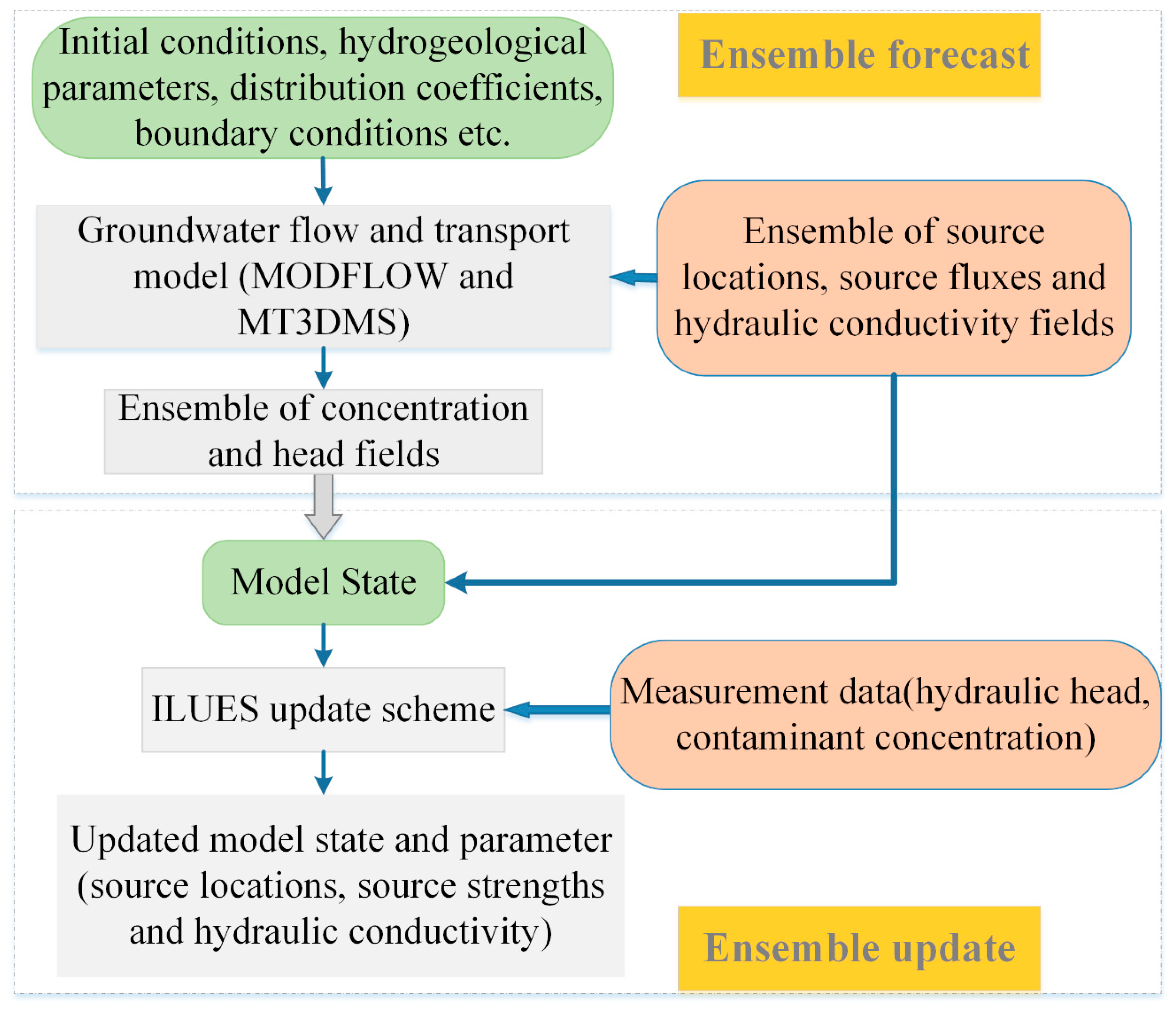
The overall procedure of the data assimilation method employing the ILUES-GEO is shown in Figure 3. The forecast stage consists of generating an ensemble of contaminant concentrations and hydraulic heads by solving groundwater flow and transport models with initial conditions, hydrogeological parameters, distribution coefficient fields, and boundary conditions via MODFLOW and MT3DMS while considering an ensemble of source locations, source strengths, and hydraulic conductivity fields. The source locations and source strengths are randomly generated based on the specific range (Table 2). The hydraulic conductivity fields are generated by KLE as stated in Section 3.1. The resulting contaminant concentrations and hydraulic heads are then regarded as the forecast results.

First, the system response variables and ensemble of source locations, source strengths, and hydraulic conductivity fields populate the forecast model state during the update stage. Second, the measurements of contaminant concentration and hydraulic head are collected from the true state. The ILUES-GEO update routine then uses the available measurements to obtain an updated estimate of the model states and parameter (source locations, source strengths, and hydraulic conductivity field).

3.3. Scenarios

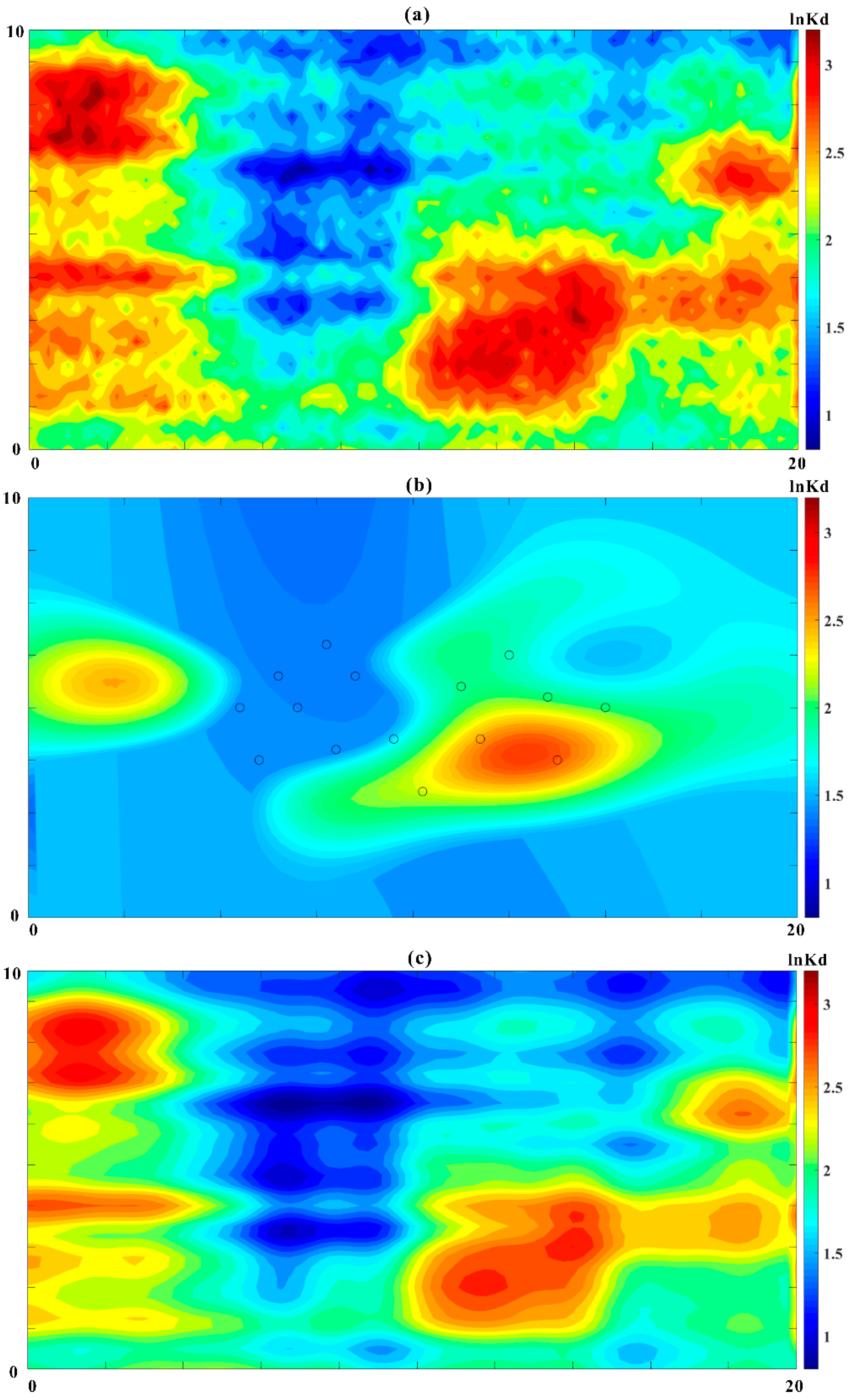
The reference distribution coefficient field is assumed to be known in this work (Figure 4b). Nevertheless, due to the contaminant characteristics and heterogeneity of the subsurface environment at real sites, sorption rates may not be the same over the entire study area when a sorption process is introduced into the solute transport model [43,44]. Moreover, the variability of the sorption strength influences the mass transfer of contaminants. The determination of the accurate sorption rate coefficients is thus essential to solve the inverse problem of groundwater contamination. This study examines three scenarios to explore the influence of the sorption rate coefficient on the estimation accuracy of the hydraulic conductivity field and source characteristics. All the other settings are the same in these three scenarios except for the sorption distribution coefficient field, and the observations are based on the reference distribution coefficient field.

In the first scenario, described in Section 3.1 as the Constant_Kd Scenario, the distribution coefficient is specified to be constant and equal to the mean value of the reference distribution coefficient field. It should be pointed out that constant distribution coefficient field is one of the most common simplified methods to tackle with solute transport model that takes sorption reaction into account [45]. Since the true sorption distribution coefficient can be obtained by fitting batch experiment results, it is an impossible task to collect all the soil samples covering the complete field to get the real distribution coefficient values. The value of a single sorption distribution coefficient from a batch experiment with several samples is always representative of the value for the entire field at real sites.

At some practical sites, only a few real parameters at specific locations (i.e., monitoring wells) are accessible throughout the field [46,47]. Generally, interpolation methods are used to produce the unknown parameter values in the rest locations based on the available true parameter values in the observed locations, which is done for simplification purposes. Consequently, in the Kringing_Kd Scenario, it is assumed that the true distribution coefficient values are available at 15 observation locations identical to those depicted in Figure 2 and that these values correspond to those in the same locations as the reference distribution coefficient field. To obtain distribution coefficient values at other locations, the Kriging method is used as an interpolation method, whose parameters are shown in

Table 4. Interpolation parameters for modeling the spatial distribution of the log-distribution coefficient in the Kriging_Kd Scenario.

	Interpolation Method	Correlation Function	Regression Model	λx[L]	λy[L]
lnKd(ln[L3/M])	Kriging	Gaussian	Zero order polynomial	5	2.5

. The simplified sorption coefficient field is shown in Figure 4b using the interpolation method.

Constant_Kd and Kringing_Kd appear to be frequent simplified ways of describing the sorption coefficient field when site heterogeneity is considered. In comparison, in the KLE_Kd Scenario, the 100 leading KLE terms are preserved to parameterize the real sorption distribution field, as detailed in Section 3.1, retaining 88% of the overall field variance. The sorption distribution coefficient field represented by the first 100 KLE terms in this scenario is depicted in Figure 4c, which is also regarded as the reference field. The corresponding parameters are also listed in Table 3, where the correlation length (λ_x and λ_y) is the same as in the Kriging_Kd Scenario.

4. Results and Discussion

4.1. Distribution Coefficient Field

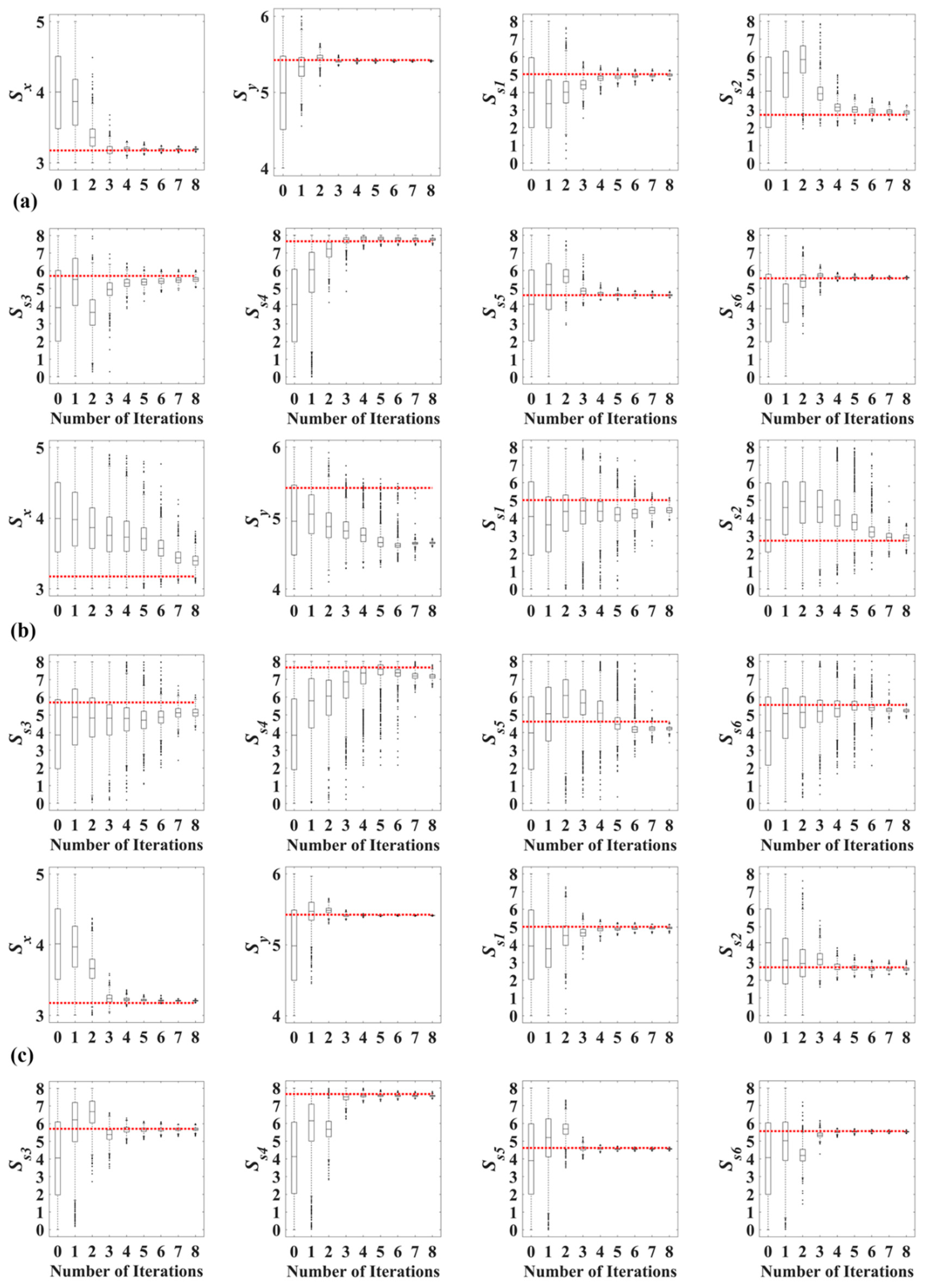
When the adsorption process is considered in the solute transport model, the sorption distribution coefficient field is difficult to characterize thoroughly due to its sparse measurements and complex nature. To demonstrate the influence of the distribution coefficient (Kd) field on the accuracy of hydraulic conductivity and source characteristics estimation, the ILUES-GEO algorithm is arranged with an ensemble size of N_e = 2000, an iteration number of N_iter = 7, a local ensemble factor of α = 0.1, and a distance weight β = 1 for the three scenarios described in Section 3.3, as suggested in Zhang et al. (2018). Figure 5 depicts the box plots of the eight source characteristics (the source location $\mathrm{coordinates}\left(S_x,S_y\right)$ and strength $S_{si},\mathrm{i}=1,\dots ,6$) versus the iteration number for Constant_Kd, Kriging_Kd, and KLE_Kd Scenario.

Note that the ILUES-GEO may accurately identify the source parameters, as illustrated in Figure 5c for KLE_Kd Scenario, whose sorption distribution coefficient is based on the reference field and is represented by 100 KLE leading terms. As shown in Figure 5a, the identified source parameters in Constant_Kd Scenario deviate substantially from the true values due to the incapacity of the constant sorption distribution coefficient across the entire site to completely represent the sorption heterogeneity. Figure 5b depicts the identification results of eight source parameters for Kriging_Kd Scenario, the performance of which is better than that of Constant_Kd Scenario but not as good as that of KLE_Kd Scenario. This may also be a result of the fact that the sorption distribution coefficient field is simplified by Kriging interpolation in Kriging_Kd Scenario, which characterizes the sorption heterogeneity to a certain degree but is limited compared with the KLE method based on the reference Kd field in this study.

The mean and variance estimates of the log-conductivity field by the ILUES-GEO algorithm for Constant_Kd, Kriging_Kd, and KLE_Kd Scenario are depicted in Figure 6, which clearly demonstrates that the similarity between the log-conductivity field obtained from KLE_Kd Scenario and the reference field is the highest, and the variance field is also the lowest. In contrast, the log-conductivity field in the center region of Constant_Kd Scenario is significantly underestimated, and the variance values are the greatest among the three Scenarios. In terms of the mean and variance field of the log-conductivity estimate, ILUES-GEO performs better in the Kriging_Kd Scenario than in Constant_Kd Scenario but worse than in the KLE_Kd Scenario (Figure 6). Consequently, the accuracy of the source characteristics identification and log-conductivity field estimate using the ILUES-GEO algorithm in the KLE_Kd Scenario is more satisfactory than that in the other two Scenarios, indicating that, on the one hand, ILUES-GEO is an efficient algorithm for solving this type of inverse problem. Moreover, the accurate representation of the heterogeneous sorption distribution coefficient field by the KLE method contributes significantly when a sorption process is introduced into the simulation model for source identification and parameter estimation.

4.2. Ensemble Size and Algorithm Factors

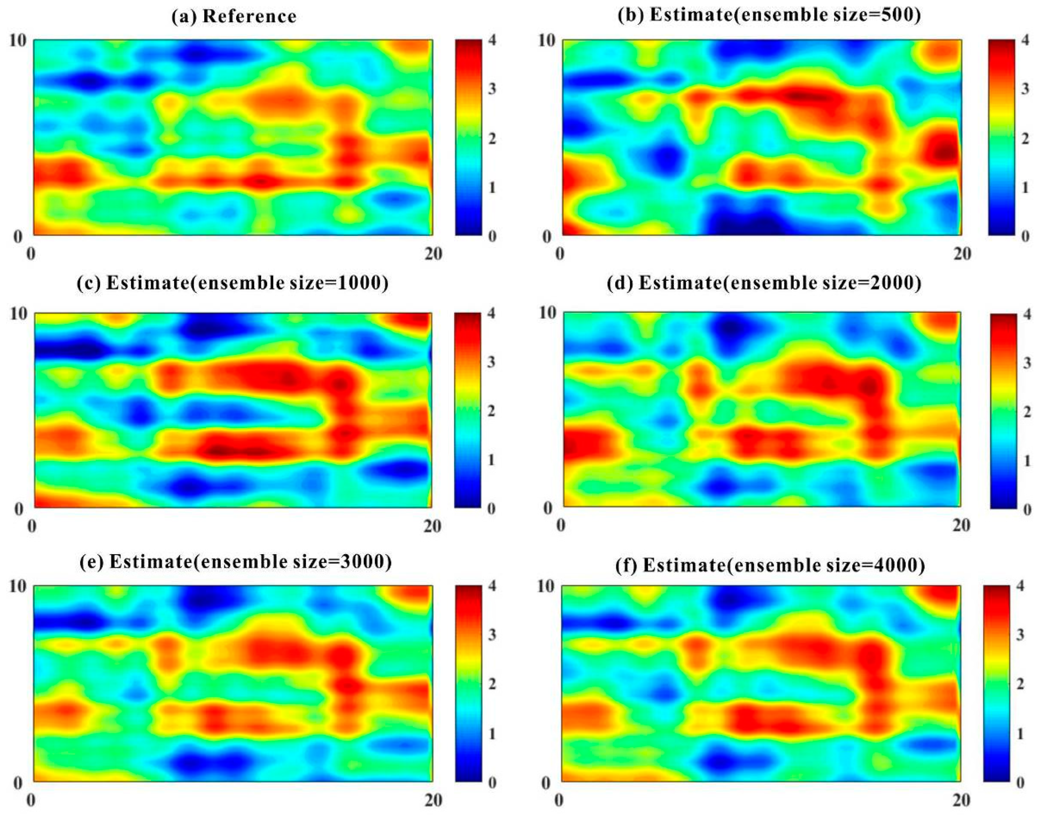
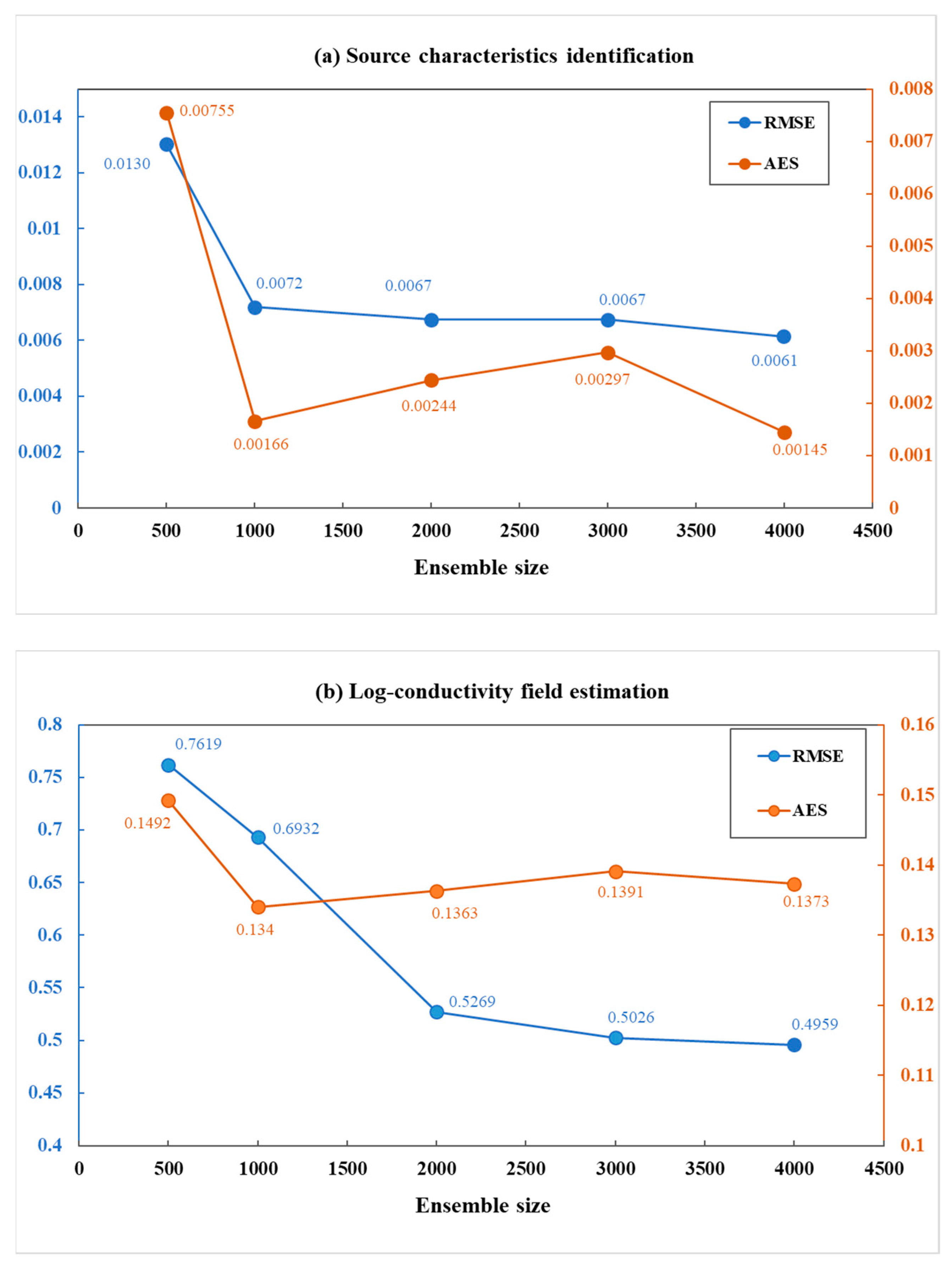
A number of assimilation runs in KLE_Kd Scenario utilizing the ILUES-GEO algorithm are executed, with ensemble sizes ranging from 500 to 4000. Specifically, the algorithm factors α and β are initially fixed to 0.1 and 1, respectively, as suggested by Zhang et al. (2018). Comparatively satisfactory results for source location and strength identification are obtained with ensemble sizes ranging from 500 to 4000, indicating that the source identification problem may be solved without employing a huge ensemble size in the ILUES-GEO algorithm. As shown in Figure 7, as the ensemble size increases from 500 to 3000, the estimation accuracy improves in comparison to the reference log-conductivity field. With larger ensembles, ILUES-GEO depicts the distribution of the log-conductivity field more accurately; thus, this is to be expected. Even while the variance of posterior realizations approaches a relatively low range as the ensemble size increases from 3000 to 4000, the performance of ILUES-GEO for estimating the log-conductivity field is barely improved.

The RMSE values for source location and strength identification are reduced by 52.82% when 4000 ensembles are used instead of 500 (Figure 8a). Similarly, the utilization of 4000 ensemble members for log-conductivity field estimation reduces the lead to RMSE values by 34.91% when compared to the use of 500 ensembles (Figure 8b). For source identification (Figure 8a) and log-conductivity estimation (Figure 8b), the AES value decreases rapidly as the ensemble size increases from 500 to 1000, whereas it fluctuates slightly and follows a similar trend without an obvious reduction when the ensemble size increases from 1000 to 4000. Another perspective to explain this variation trend is that enlarging AES values enables the smoother (ILUES-GEO) to correct estimated errors in the subsequent assimilation iteration (Gharamti et al., 2014). As the number of ensemble members exceeds 4000, the AES value gradually stabilizes at 0.00145 and 0.4959, respectively, following ILUES-GEO assimilation for source identification and log-conductivity estimation. Note that the CPU time and storage required to execute the ILUES-GEO assimilation scheme with 4000 ensembles may be considerably higher than when only 500 ensembles are used. To strike a balance between computational efficiency and accuracy, an ensemble size of 2000 might be an appropriate choice for this study.

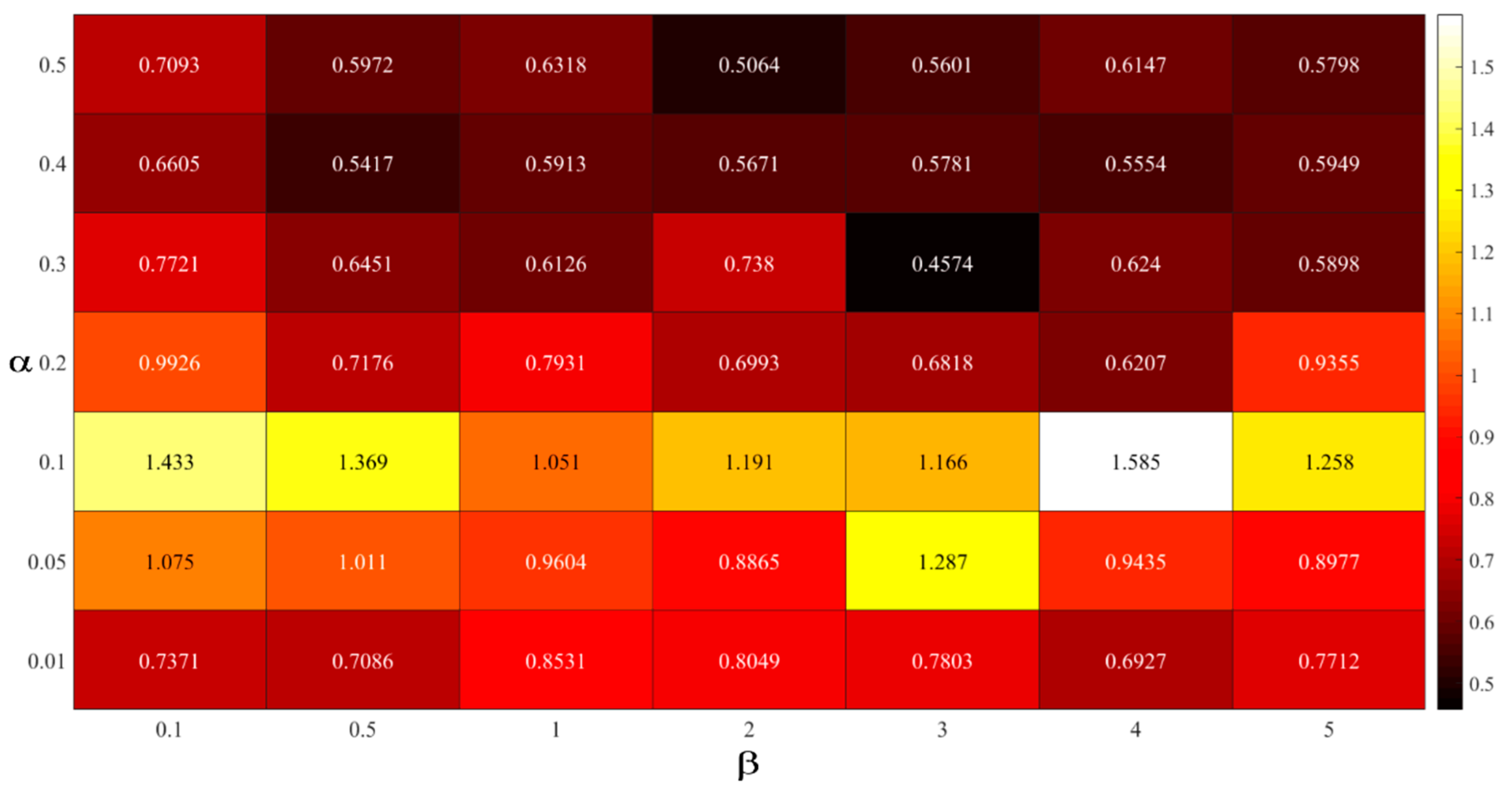
The ILUES-GEO system is used to estimate source information and hydraulic conductivity fields under the same modeling conditions with the sorption parameter field in the KLE_Kd Scenario. Two factors mentioned in Section 2.2.2 must be assigned to the ILUES-GEO scheme: α (the ratio between local and global ensemble) and β (a factor assigning different weights to the two normalized distances). To save computational time, an ensemble size of 500 is chosen for these assimilation runs. A total of 49 assimilation runs are conducted, in which varying candidates for α (0.01, 0.05, 0.1, 0.2, 0.3, 0.4, 0.5) and β (0.1, 0.5, 1, 2, 3, 4, 5) are selected to determine the influence of these factors on the performance of the ILUES-GEO algorithm.

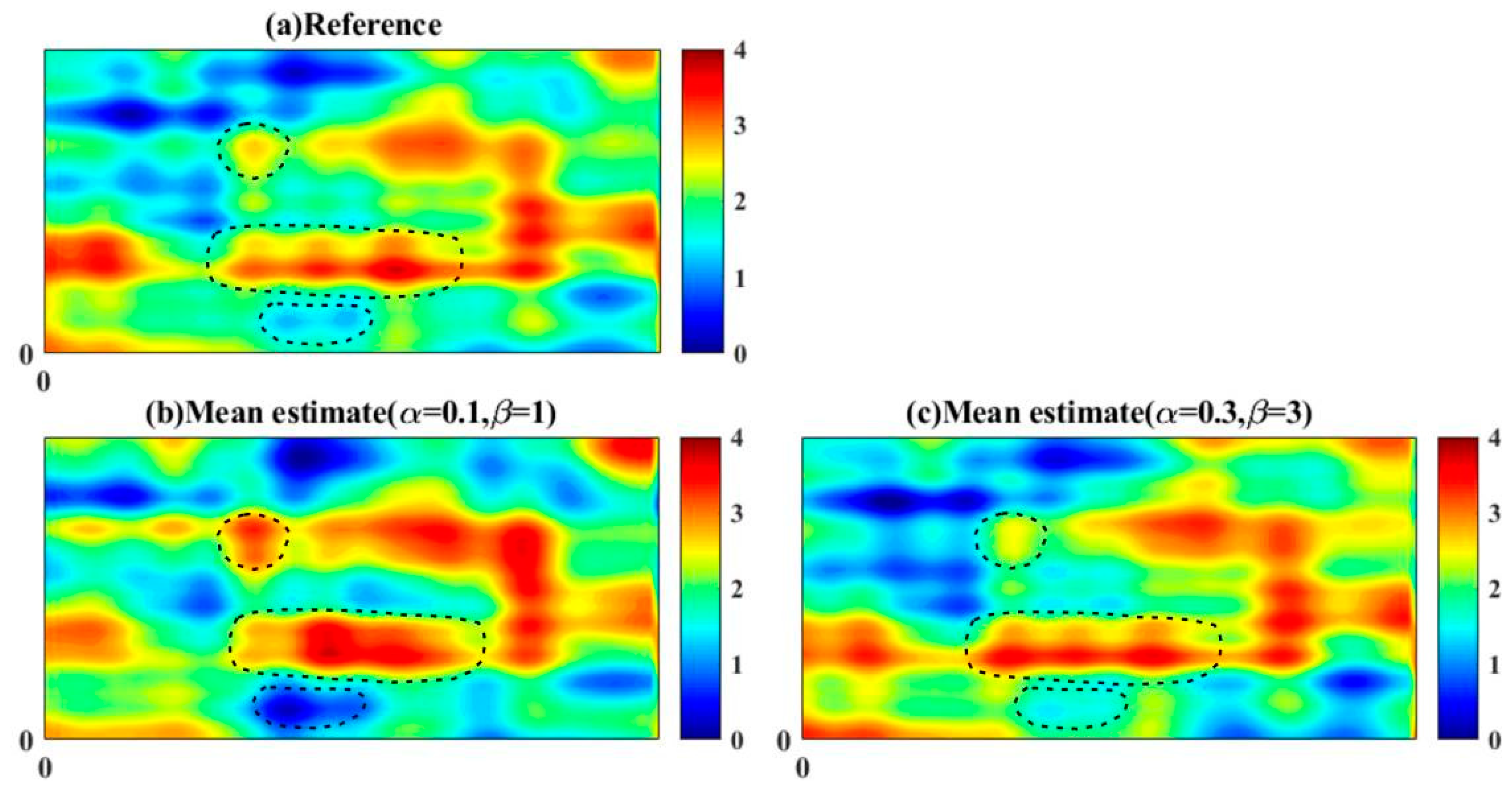
The resulting RMSE values of the log-conductivity field estimations are shown in Figure 9. When α is held constant across a range of β values, the RMSE values change marginally. Optimal α values for this problem with fixing β range between 0.3 and 0.5. Furthermore, the lowest RMSE value is obtained for α = 0.3 and β = 3 for this case, which indicates that 30% of the global ensemble is preserved as the local ensemble and that the parametric distance is 3 times the weight of the model response distance, respectively. Consistent with the findings of Zhang et al. (2018), a relatively large β value (e.g., β > 0.1) is needed when α ≥ 0.1. On the other hand, a greater weight is assigned to the parametric distance in this situation, demonstrating that the attributes of the local ensemble closer to the sample matter more to measurements in this case. The log-conductivity field estimation result of the ILUES-GEO algorithm with optimal factors α = 0.3 and β = 3 is compared with the result of the ILUES-GEO method with proposed factors α = 0.1 and β = 1 by Zhang et al.(2018) in Figure 10. Both mean estimates resulting from ILUES-GEO with α = 0.1, β = 1 (Figure 10b) and α = 0.3, β = 3 (Figure 10c) accurately map the spatial patterns of the reference log-conductivity field and identify source characteristics. The main low and high conductivity zones are well captured by ILUES-GEO with α = 0.3 and β = 3, especially the middle zones (region with black dashed line) of the domain depicted in Figure 10, whereas ILUES-GEO depicts these zones inadequately with α = 0.1 and β = 1. In addition, the RMSE values of hydraulic conductivity field estimation obtained from ILUES with α = 0.1, β = 1 and α = 0.3, β = 3 are 0.5184 and 0.4258, respectively, which also demonstrates that the ILUES-GEO with factors α = 0.3 and β = 3 for this problem performs better than that with α = 0.1 and β = 1.

4.3. Observation Number and Location

As in the aforementioned sections, groundwater head and contaminant concentration observation locations are assembled in the main contaminant plume area in the catchment. Head measurements are taken once at 15 points as shown in Figure 2, while contaminant concentration measurements are gathered from time steps 5 to 13. The measurements at different observation locations are impacted by the diffusion and sorption processes of contaminant transport. It is thus required to investigate the effect of head and contaminant concentration measurement locations and numbers on the data assimilation performance of the ILUES-GEO scheme for the source information and system parameter estimation problem.

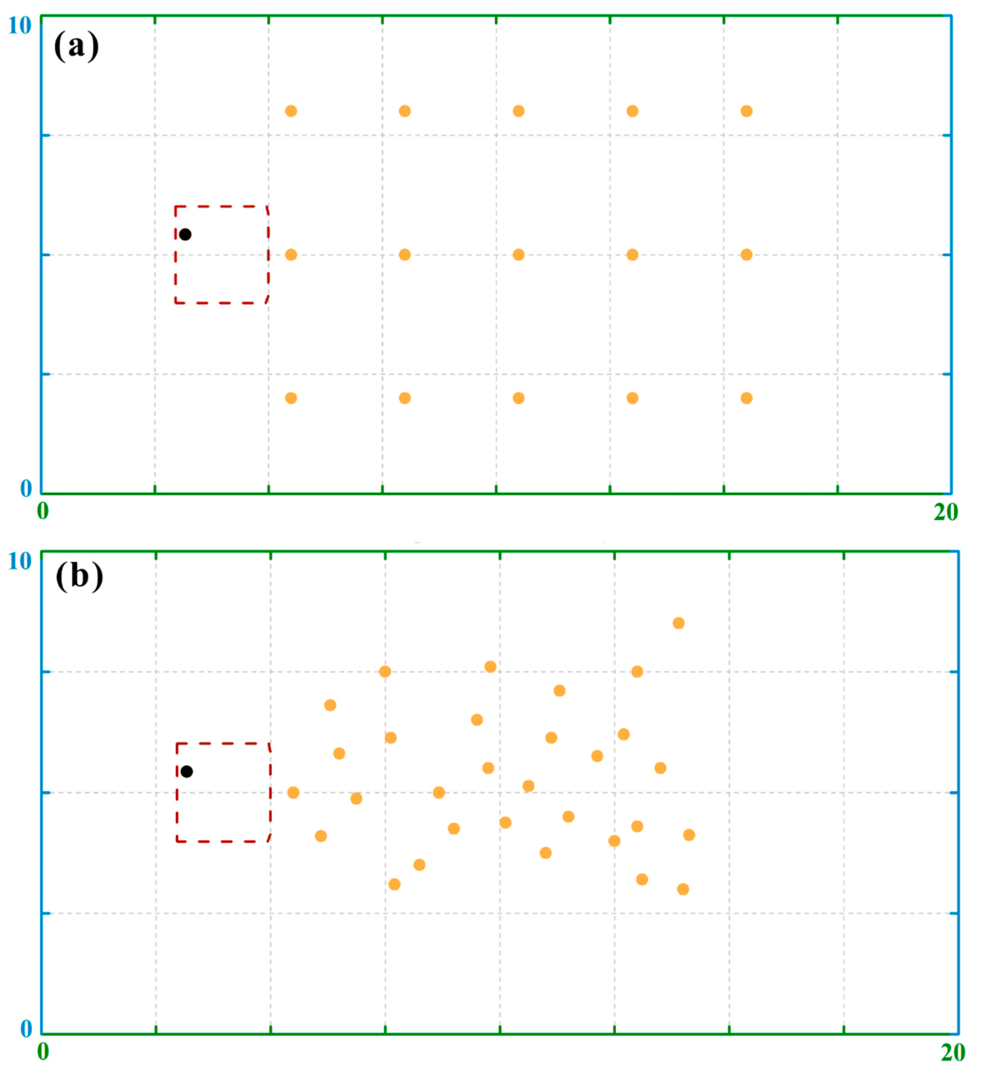
Using the ILUES-GEO algorithm with an ensemble size of 2000, an iteration number of 8, and factors of α = 0.3 and β = 3, respectively, three different patterns of measurement locations are introduced to the KLE_Kd Scenario. The same number of 15 observation locations with two different distribution patterns are displayed in Figure 2 and Figure 11a, where the observations are randomly distributed in a zone with relatively obvious variation of contaminant concentration and sparsely distributed uniformly, respectively. In addition, 30 randomly distributed observations are shown in Figure 11b within the main contaminant plume.

After the assimilation procedure of the ILUES-GEO, the box plots of the identification results for eight source characteristics (the source location coordinates $\left(S_x,S_y\right)$ and strength $S_{si},\mathrm{i}=1,\dots ,6$) versus the iteration number for three different observation patterns are plotted in Figure 12. Moreover, Figure 13 depicts the resulting mean estimate and variance of log-hydraulic conductivity fields with various observation settings. We first investigate the influence of observation locations on the performance of ILUES-GEO in this scenario. The ILUES-GEO scheme assimilating the hydraulic head and contaminant concentration data from 15 random observation locations in the main contaminant plume (Figure 2) clearly outperforms the ILUES-GEO scheme assimilating the data from 15 uniformly distributed observation locations in terms of the identification results of source characteristics involving source locations and source strengths shown in Figure 12a,b. In contrast to the estimation results of the hydraulic parameters in Figure 13d,e using the uniform observation pattern of Figure 11a, assimilating data from the random observation pattern of Figure 2 resulted in a more accurate mean estimate of log-conductivity and a lower variance field shown in Figure 13b,c. This is because the randomly distributed observations in Figure 2 are mainly located in the zone where the contaminant concentration varies obviously in the study domain, and the observed concentration in the first and third rows of the observations in Figure 11a might be too low to be useful in the data assimilation scheme and to capture the variation in contaminant concentration.

To explore the impact of the number of observation locations on the joint estimation of source information and hydraulic parameters, the ILUES-GEO algorithm is employed to assimilate data from 15 and 30 randomly distributed observation locations in the similar area of the study domain, as shown in Figure 2 and Figure 11b, respectively. Figure 12b,c indicate that the source characteristics can be identified accurately by ILUES-GEO using the hydraulic head and contaminant concentration data from 15 and 30 observation locations (Figure 2 and Figure 11b). However, for the strengths $S_{s2}$ and $S_{s3}$, ILUES-GEO with 30 observations yields identification values that are more accurate and have fewer uncertainties. As shown in Figure 13b,f, the major low and high log-hydraulic conductivity zones are well captured by assimilating data from 15 observation locations (Figure 2), whereas the assimilation results using 30 observation locations (Figure 11b) could better represent these structures, particularly the northwest low-conductivity zone and the southeast high-conductivity corner of the study domain. The assimilation of the data from 30 observation locations yielded a field of estimated log-hydraulic conductivity with a smaller variance (Figure 13g) in comparison with the assimilation of data from 15 observation locations (Figure 13c).

The above study results indicate that both the location and number of observations influence the performance of the joint estimation of the source characteristics and hydraulic conductivity field by the ILUES-GEO algorithm. The optimal combination of the observation number and locations may enhance the accuracy of inverse results. How to design the optimal number and locations of observations in advance for source identification and parameter estimation is beyond the scope of this study and is worth being investigated in further research.

5. Conclusions

In this study, an iterative local updating ensemble smoother with geometric inflation selection is employed to assimilate the hydraulic head and contaminant concentration measurements to jointly estimate the hydraulic conductivity field and contaminant source characteristics in a two-dimensional heterogeneous aquifer with different sorption parameter settings. Three scenarios with different simplification methods of the sorption distribution coefficient field are presented to investigate the applicability of the ILUES-GEO scheme and the effect of sorption parameter setting on the identification of contaminant source information and the estimation of hydraulic conductivity. In the first scenario, the sorption parameter is determined as a constant. In the second scenario, the sorption parameter field is defined using the Kriging interpolation method based on the sorption parameters available at the specific observation locations. In the last scenario, the Karhunen–Loève expansion method is adopted to present the sorption parameter field as the reference field to preserve more uncertainties. To improve the performance of the ILUES-GEO scheme in this problem, sensitivity numerical tests involving ensemble size and the algorithm parameters α and β are also implemented. The number and location of observations are discussed to further explore their impacts on the estimation results.

The following conclusions are drawn based on the study results:

• The ILUES-GEO scheme is employed to estimate the hydraulic conductivity field and contaminant source information when the sorption process is considered in a solute transport model by assimilating hydraulic head and contaminant concentration measurements. After a few iterations, the contaminant source characteristics are identified in terms of source locations and source strengths, and the spatial distribution of hydraulic conductivity approaches the distribution of the reference field.
• The KLE_Kd Scenario, in which the sorption parameter field is represented by the Karhunen–Loève expansion method as the reference field rather than simplified by Kriging interpolation or a constant value, yields the best performance of ILUES-GEO in terms of both the estimative performance of hydraulic conductivity and the identified performance of contaminant source information, as indicated by the decreasing variance and similar distribution of hydraulic conductivity to the reference field and the closer values of source characteristics to the true ones. The accurate determination of the sorption parameter field is essential to characterize the heterogeneity of the subsurface and jointly estimate hydraulic parameters and source characteristics.
• The ILUES-GEO scheme can obtain increasingly accurate estimations of both source characteristics and the hydraulic conductivity field as the ensemble size increases. Furthermore, an excessively high ensemble size may result in a heavy computational burden, and the sensitivity of the estimation results to ensemble size gets weak. The ensemble size of 2000 is sufficient for this study to provide satisfactory results.
• The settings for factors α and β have an impact on the performance of the ILUES-GEO scheme. α and β represent the ratio of the local ensemble to the global and the weight assigned to the two distances, comprising the distance between the model results and observations and the distance between the model parameters and samples, respectively. The results of numerical experiments suggest that the combination of α = 0.3 and β = 3 is the optimal factor setting for the ILUES-GEO algorithm in this study.
• The number and location of observation points influence the results of parameter estimation and source identification using the ILUES-GEO algorithm. The ILUES-GEO system performs better under certain conditions as the number of observations grows. Observations positioned in the region where obvious variations of hydraulic head and contaminant concentration are captured may help to obtain more accurate joint estimation results for this study. Further research is necessary to determine the optimal number and design of observation locations for different cases.

References

1. Barrios, R.E.; Gaonkar, O.; Snow, D.; Li, Y.; Bartelt-Hunt, S.L. Enhanced biodegradation of atrazine at high infiltration rates in agricultural soils. Environ. Sci. Process Impacts 2019, 21, 999–1010. [Google Scholar] [CrossRef] [PubMed]
2. Famisan, G.B.; Brusseau, M.L. Biodegradation during contaminant transport in porous media: 6. Impact of sorption on coupled degradation-transport behavior. Environ. Toxicol. Chem. 2003, 22, 510–517. [Google Scholar] [CrossRef] [PubMed]
3. Maier, R.M. Biological Processes Affecting Contaminants Transport and Fate. In Environmental and Pollution Science, 3rd ed.; Academic Press: Cambridge, MA, USA, 2019; pp. 131–146. [Google Scholar] [CrossRef]
4. Cunningham, J.A.; Roberts, P.V. Use of temporal moments to investigate the effects of nonuniform grain-size distribution on the transport of sorbing solutes. Water Resour. Res. 1998, 34, 1415–1425. [Google Scholar] [CrossRef]
5. Zhang, X.; Ma, F.; Yin, S.; Wallace, C.D.; Lü, X. Application of upscaling methods for fluid flow and mass transport in multi-scale heterogeneous media: A critical review. Appl. Energ. 2021, 303, 117603. [Google Scholar] [CrossRef]
6. Haggerty, R.; Harvey, C.F.; Von Schwerin, C.F.; Meigs, L.C. What controls the apparent timescale of solute mass transfer in aquifers and soils? A comparison of experimental results. Water Resour. Res. 2004, 40, W01510. [Google Scholar] [CrossRef] [Green Version]
7. Gharamti, M.E.; Valstar, J.; Hoteit, I. An adaptive hybrid EnKF-OI scheme for efficient state-parameter estimation of reactive contaminant transport models. Adv. Water Resour. 2014, 71, 1–15. [Google Scholar] [CrossRef]
8. Gharamti, M.E.; Ait-El-Fquih, B.; Hoteit, I. An iterative ensemble Kalman filter with one-step-ahead smoothing for state-parameters estimation of contaminant transport models. J. Hydrol. 2015, 527, 442–457. [Google Scholar] [CrossRef] [Green Version]
9. Kitanidis, P.K. Persistent questions of heterogeneity, uncertainty, and scale in subsurface flow and transport. Water Resour. Res. 2015, 51, 5888–5904. [Google Scholar] [CrossRef]
10. Michael, C.H.; Marco, I.; Paul, W.; Oliver, K.; Jonathan, C.; Andrew, B. Efficient multi-scale imaging of subsurface resistivity with uncertainty quantification using ensemble Kalman inversion. Geophys. J. Int. 2021, 225, 887–905. [Google Scholar] [CrossRef]
11. Ju, L.; Zhang, J.; Chen, C.; Wu, L.; Zeng, L. Water flux characterization through hydraulic head and temperature data assimilation: Numerical modeling and sandbox experiments. J. Hydrol. 2018, 558, 104–114. [Google Scholar] [CrossRef]
12. Huang, Q.; Qin, G.; Zhang, Y.; Tang, Q.; Post, D. Using Remote Sensing Data-based Hydrological Model Calibrations for Predicting Runoff in Ungauged or Poorly Gauged Catchments. Water Resour. Res. 2020, 56, e2020WR028205. [Google Scholar] [CrossRef]
13. Ghorbanidehno, H.; Kokkinaki, A.; Lee, J.; Darve, E. Recent developments in fast and scalable inverse modeling and data assimilation methods in hydrology. J. Hydrol. 2020, 591, 125266. [Google Scholar] [CrossRef]
14. Kang, X.; Shi, X.; Revil, A.; Cao, Z.; Wu, J. Coupled hydrogeophysical inversion to identify non-Gaussian hydraulic conductivity field by jointly assimilating geochemical and time-lapse geophysical data. J. Hydrol. 2019, 578, 124092. [Google Scholar] [CrossRef]
15. Lan, T.; Shi, X.; Jiang, B.; Sun, Y.; Wu, J. Joint inversion of physical and geochemical parameters in groundwater models by sequential ensemble-based optimal design. Stoch. Environ. Res. Risk Assess. 2018, 32, 1919–1937. [Google Scholar] [CrossRef]
16. Pleasants, M.S.; Neves, F.; Parsekian, A.D.; Befus, K.M.; Kelleners, T.J. Hydrogeophysical Inversion of Time-Lapse ERT Data to Determine Hillslope Subsurface Hydraulic Properties. Water Resour. Res. 2022, 58, 2021WR031073. [Google Scholar] [CrossRef]
17. Ju, L.; Zhang, J.; Meng, L.; Wu, L.; Zeng, L. An adaptive Gaussian process-based iterative ensemble smoother for data assimilation. Adv. Water Resour. 2018, 115, 125–135. [Google Scholar] [CrossRef]
18. Lei, L.; Wang, Z.; Tan, Z.M. Integrated Hybrid Data Assimilation for an Ensemble Kalman Filter. Mon. Weather Rev. 2021, 149, 4091–4105. [Google Scholar] [CrossRef]
19. Zhang, J.; Lin, G.; Li, W.; Wu, L.; Zeng, L. An Iterative Local Updating Ensemble Smoother for Estimation and Uncertainty Assessment of Hydrologic Model Parameters with Multimodal Distributions. Water Resour. Res. 2018, 54, 1716–1733. [Google Scholar] [CrossRef]
20. Zhang, S.; Liu, Z.; Zhang, X.; Wu, X.; Deng, X. Coupled data assimilation and parameter estimation in coupled ocean–atmosphere models: A review. Clim. Dynam. 2020, 54, 5127–5144. [Google Scholar] [CrossRef]
21. Zheng, Q.; Zhang, J.; Xu, W.; Wu, L.; Zeng, L. Adaptive Multifidelity Data Assimilation for Nonlinear Subsurface Flow Problems. Water Resour. Res. 2019, 55, 203–217. [Google Scholar] [CrossRef] [Green Version]
22. Evensen, G. The Ensemble Kalman Filter: Theoretical formulation and practical implementation. Ocean Dyn. 2003, 53, 343–367. [Google Scholar] [CrossRef]
23. Hendricks Franssen, H.J.; Kinzelbach, W. Real-time groundwater flow modeling with the Ensemble Kalman Filter: Joint estimation of states and parameters and the filter inbreeding problem. Water Resour. Res. 2008, 44, 1–21. [Google Scholar] [CrossRef]
24. Houtekamer, P.L.; Zhang, F. Review of the ensemble Kalman filter for atmospheric data assimilation. Mon. Weather Rev. 2016, 144, 4489–4532. [Google Scholar] [CrossRef]
25. Keller, J.; Franssen, H.; Nowak, W. Investigating the Pilot Point Ensemble Kalman Filter for geostatistical inversion and data assimilation. Adv. Water Resour. 2021, 155, 104010. [Google Scholar] [CrossRef]
26. Sun, Y.; Bao, W.; Valk, K.; Brauer, C.C.; Sumihar, J.; Weerts, A.H. Improving forecast skill of lowland hydrological models using ensemble Kalman filter and unscented Kalman filter. Water Resour. Res. 2020, 56, 2020WR027468. [Google Scholar] [CrossRef]
27. Zhou, H.; Gómez-Hernández, J.J.; Hendricks Franssen, H.J.; Li, L. An approach to handling non-Gaussianity of parameters and state variables in ensemble Kalman filtering. Adv. Water Resour. 2011, 34, 844–864. [Google Scholar] [CrossRef] [Green Version]
28. Van Leeuwen, P.J.; Evensen, G. Data assimilation and inverse methods in terms of a probabilistic formulation. Mon. Weather Rev. 1996, 124, 2898–2913. [Google Scholar] [CrossRef]
29. Li, L.; Stetler, L.; Cao, Z.; Davis, A. An iterative normal-score ensemble smoother for dealing with non-Gaussianity in data assimilation. J. Hydrol. 2018, 567, 759–766. [Google Scholar] [CrossRef]
30. Todaro, V.; D’Oria, M.; Tanda, M.G.; Gómez-Hernández, J.J. Ensemble smoother with multiple data assimilation to simultaneously estimate the source location and the release history of a contaminant spill in an aquifer. J. Hydrol. 2021, 598, 126215. [Google Scholar] [CrossRef]
31. Bailey, R.; Baù, D. Ensemble smoother assimilation of hydraulic head and return flow data to estimate hydraulic conductivity distribution. Water Resour. Res. 2010, 46, 1–19. [Google Scholar] [CrossRef]
32. Skjervheim, J.A.; Evensen, G. An ensemble smoother for assisted history matching. Soc. Pet. Eng. SPE Reserv. Simul. Symp. 2011, 2, 1049–1063. [Google Scholar] [CrossRef]
33. Pansa, A.; Butera, I.; Gómez-Hernández, J.J.; Vigna, B. Predicting discharge from a complex karst system using the ensemble smoother with multiple data assimilation. Stoch. Environ. Res. Risk Assess. 2022; in press. [Google Scholar] [CrossRef]
34. Emerick, A.A.; Reynolds, A.C. Ensemble smoother with multiple data assimilation. Comput. Geosci. 2013, 55, 3–15. [Google Scholar] [CrossRef]
35. Forouzanfar, F.; Wu, X.H. Constrained iterative ensemble smoother for multi solution search assisted history matching. Comput. Geosci. 2021, 25, 1593–1604. [Google Scholar] [CrossRef]
36. Mo, S.; Zabaras, N.; Shi, X.; Wu, J. Deep Autoregressive Neural Networks for High-Dimensional Inverse Problems in Groundwater Contaminant Source Identification. Water Resour. Res. 2019, 55, 3856–3881. [Google Scholar] [CrossRef] [Green Version]
37. Emerick, A.A. Analysis of geometric selection of the data-error covariance inflation for ES-MDA. J. Pet. Sci. Eng. 2019, 182, 106168. [Google Scholar] [CrossRef] [Green Version]
38. Cvetkovic, V.; Dagan, G.; Cheng, H. Contaminant transport in aquifers with spatially variable hydraulic and sorption properties. Proc. R. Soc. A Math. Phys. Eng. Sci. 1998, 454, 2173–2207. [Google Scholar] [CrossRef]
39. Nair, V.V. Influence of colloid and adsorption parameters on contaminant transport in fractured rocks—A triple continuum model. Groundw. Sustain. Dev. 2019, 8, 381–389. [Google Scholar] [CrossRef]
40. You, X.; Liu, S.; Dai, C.; Guo, Y.; Duan, Y. Contaminant occurrence and migration between high- and low-permeability zones in groundwater systems: A review. Sci. Total Environ. 2020, 743, 140703. [Google Scholar] [CrossRef] [PubMed]
41. Yang, S.-F.; Lin, C.-F.; Yu-Chen, L.A.; Andy Hong, P.-K. Sorption and biodegradation of sulfonamide antibiotics by activated sludge: Experimental assessment using batch data obtained under aerobic conditions. Water Res. 2011, 45, 3389–3397. [Google Scholar] [CrossRef]
42. Zhang, D.; Lu, Z. An efficient, high-order perturbation approach for flow in random porous media via Karhunen-Loève and polynomial expansions. J. Comput. Phys. 2004, 194, 773–794. [Google Scholar] [CrossRef]
43. Allen-King, R.M.; Halket, R.M.; Gaylord, D.R.; Robin, M.J.L. Characterizing the heterogeneity and correlation of perchloroethene sorption and hydraulic conductivity using a facies-based approach. Water Resour. Res. 1998, 34, 385–396. [Google Scholar] [CrossRef]
44. Chen, W.; Wagenet, R.J. Solute Transport in Porous Media with Sorption-Site Heterogeneity. Environ. Sci. Technol. 1995, 29, 2725–2734. [Google Scholar] [CrossRef] [PubMed]
45. Chongxuan, L.; Ball, W.P. Application of inverse methods to contaminant source identification from aquitard diffusion profiles at Dover AFB, Delaware. Water Resour. Res. 1999, 35, 1975–1985. [Google Scholar] [CrossRef]
46. Gailichand, J.; Prasher, S.O.; Broughton, R.S.; Marcotte, D. Kriging of hydraulic conductivity for subsurface drainage design. J. Irrig. Drain. Eng. 1991, 117, 667–681. [Google Scholar] [CrossRef]
47. Motaghian, H.R.; Mohammadi, J. Spatial estimation of saturated hydraulic conductivity from terrain attributes using regression, kriging, and artificial neural networks. Pedosphere 2011, 21, 170–177. [Google Scholar] [CrossRef]
Figure 1. Flowchart of the ILUES-GEO algorithm.
Sustainability 15 01211 g001
Figure 2. Flow domain of the study area and spatial maps of the reference log-conductivity field considered in this study. The black dot and the dark red dashed rectangle denote the contaminant source and potential area of the source, respectively. The hollow circles denote the observation locations.
Sustainability 15 01211 g002
Figure 3. Flowchart of data assimilation scheme.
Sustainability 15 01211 g003
Figure 4. The spatial maps of sorption distribution coefficient: (a) Reference field; (b) Kriging_Kd Scenario; (c) KLE_Kd Scenario. The black circles in (b) denote specific locations for available real sorption coefficient.
Sustainability 15 01211 g004
Figure 5. Source location and source strength box plots for each iteration for (a) Constant_Kd Scenario, (b) Kriging_Kd Scenario, and (c) KLE_Kd Scenario. The horizontal red dot lines represent the true values of source characteristics.
Sustainability 15 01211 g005
Figure 6. The reference log-conductivity field (a) and estimated mean and variance fields for Constant_Kd Scenario (b,c), Kriging_Kd Scenario (d,e), and KLE_Kd Scenario (g,f).
Sustainability 15 01211 g006
Figure 7. The reference log-conductivity field and estimated fields with different ensemble sizes in KLE_Kd Scenario, (a): Reference log-conductivity field; (b): Ensemble size = 500; (c): Ensemble size = 1000; (d): Ensemble size = 2000; (e): Ensemble size = 3000; (f): Ensemble size = 4000.
Sustainability 15 01211 g007
Figure 8. RMSE (blue dots) and AES (orange dots) values resulting from the ILUES with different ensemble sizes, (a): for source location and source strength identification; (b): for log-conductivity field estimation.
Sustainability 15 01211 g008
Figure 9. RMSE values of log-conductivity field estimation using the ILUES scheme with different combinations of factor α and β.
Sustainability 15 01211 g009
Figure 10. Reference and the mean estimates of log-conductivity field resulting from ILUES algorithm with different factors α and β. (a) reference log-conductivity field; (b) mean estimate of log-conductivity field using ILUES with α = 0.1, β = 1; (c) mean estimate of log-conductivity field using ILUES with α = 0.3, β = 3.
Sustainability 15 01211 g010
Figure 11. The distribution patterns for observation wells: (a) 15 observation wells distributed uniformly; (b) 30 observation wells distributed randomly in relatively high contaminant concentration zone. The black dot and the dark red dashed rectangle denote the contaminant source and the potential source area, respectively. The orange dots denote the observation locations.
Sustainability 15 01211 g011
Figure 12. Box plots of the source location coordinates and source strength at each iteration for KLE_Kd Scenario with different patterns of observations: (a) 15 observations randomly distributed in the relatively high concentration zone, (b) 15 observations uniformly distributed in the domain, (c) 30 observations randomly distributed in the relatively high concentration zone. The horizontal dotted red lines denote the true values of source characteristics.
Sustainability 15 01211 g012
Figure 13. The reference log-conductivity field (a) and estimated mean and variance fields for KLE_Kd Scenario with different patterns of observations: (b,c) 15 observations randomly distributed in the relatively high concentration zone, (d,e) 15 observations uniformly distributed in the domain, (f,g) 30 observations randomly distributed in the relatively high concentration zone.
Sustainability 15 01211 g013