
Conceptual Framework for Modelling of an Electric Tractor and Its Performance Analysis Using a Permanent Magnet Synchronous Motor

Abstract
:1. Introduction
2. Literature Review
3. Mathematical Modelling
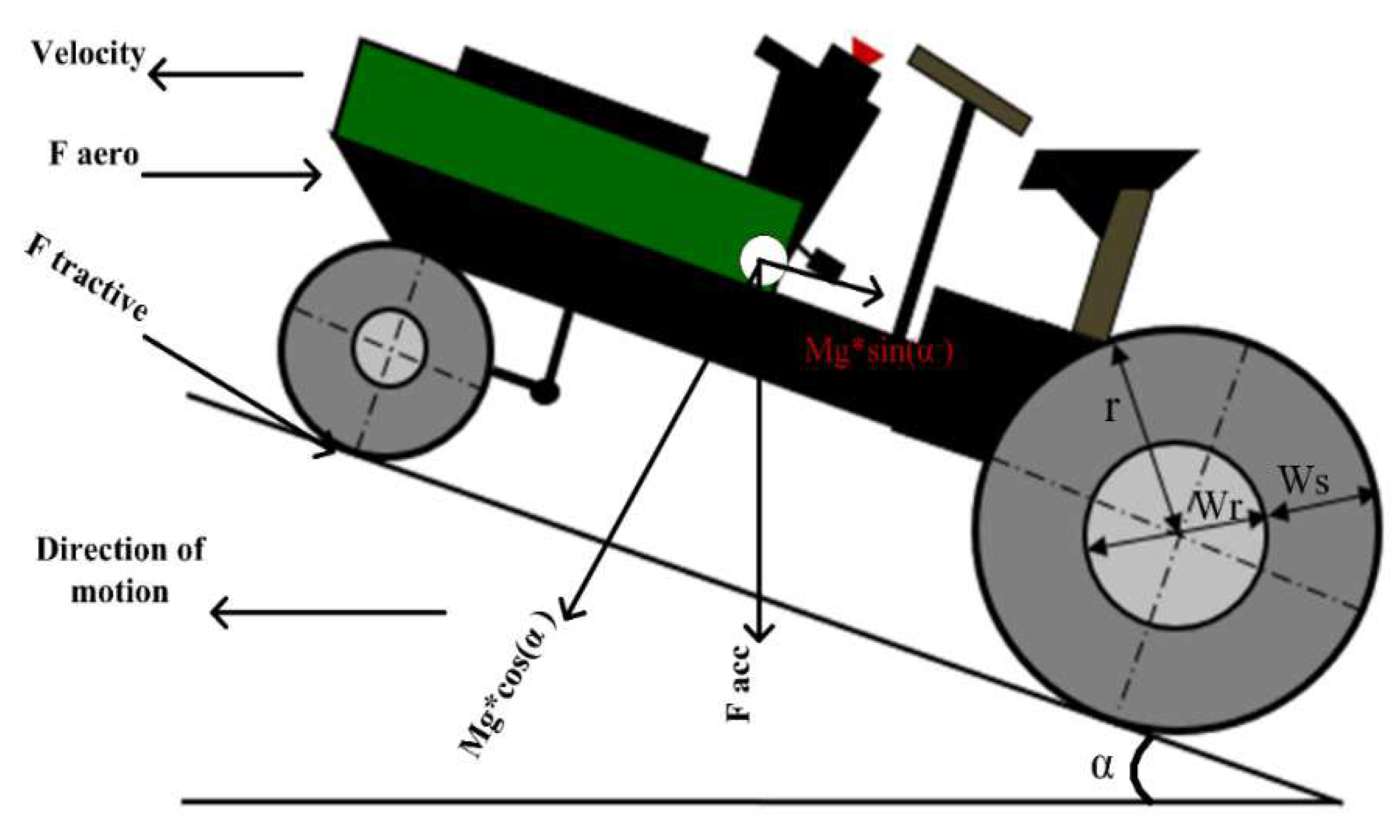
3.1. Modelling of Electric Tractor (ET)
3.1.1. Rolling Resistance Force
3.1.2. Aero Dynamic Drag Force
3.1.3. Gradient Force
3.1.4. Acceleration Force
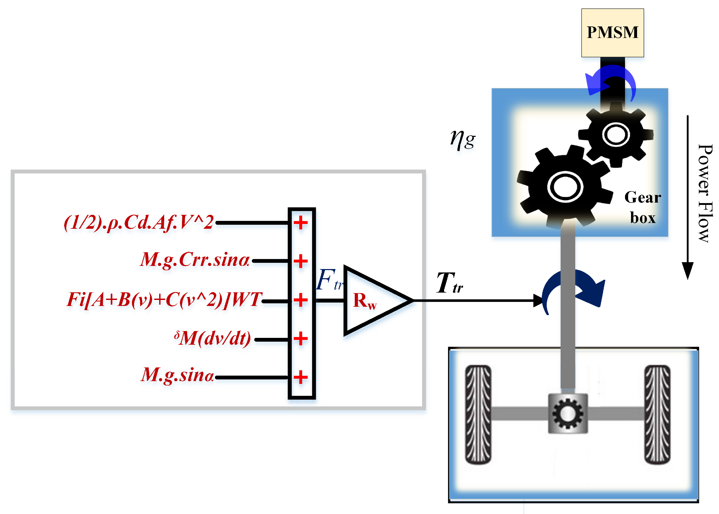
3.1.5. Drawbar Force
- Fi = soil texture adjustment parameter (dimensionless);
- i = 1 for fine, 2 for medium, and 3 for coarse-textured soils (dimensionless);
- A, B, and C = machine-specific parameters (dimensionless);
- V = field speed (km h−1);
- W = machine width (m or number of rows or tools);
- T = tillage depth (cm) for major tools or 1 (dimensionless) for minor tillage tools and seeding implements.
3.1.6. Total Tractive Effort
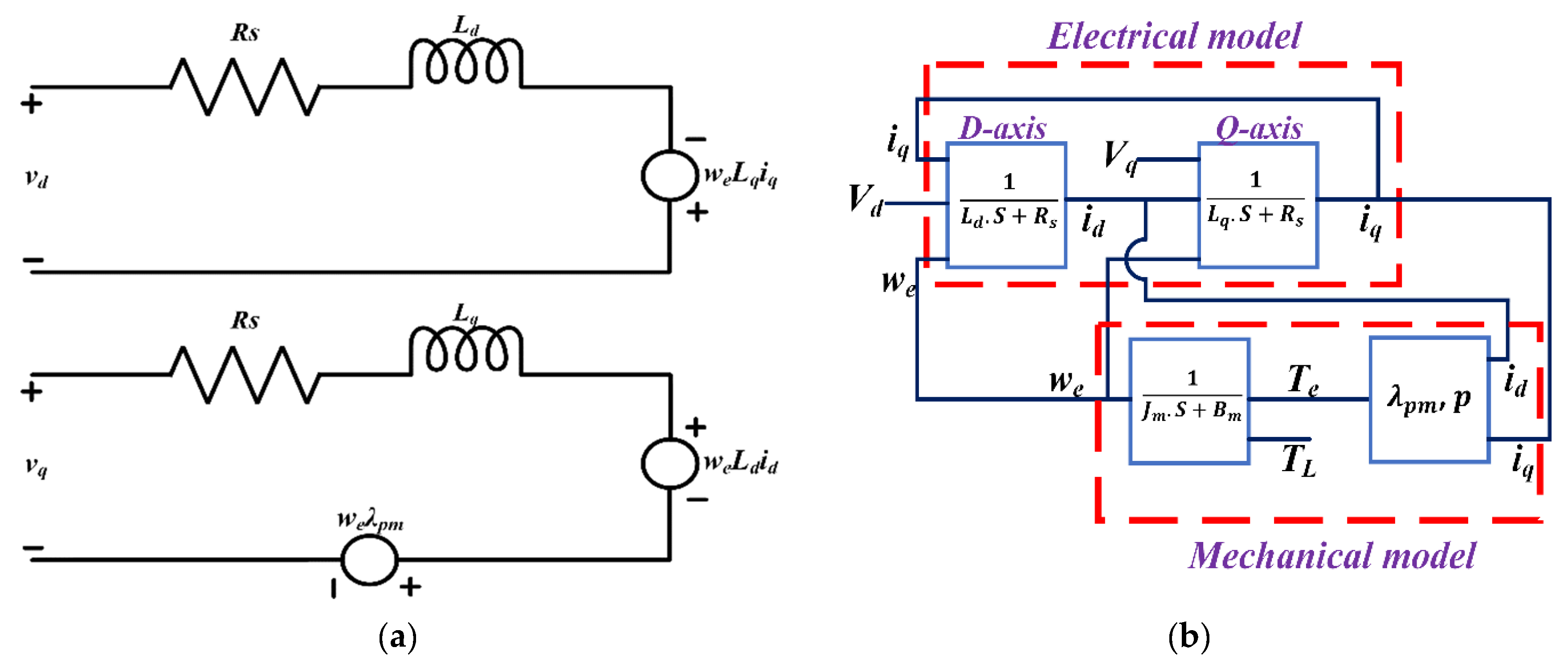
3.2. Mathematical Modelling of PMSM
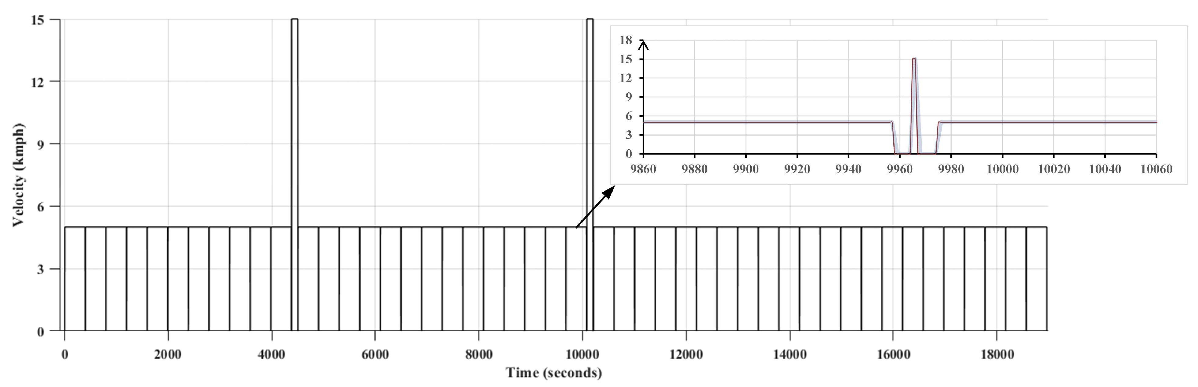
3.3. Working Condtions and Loadprofile Modelling
4. Proposed Methodology
4.1. Tractor Load Simulation Using Dynamometer
4.2. Control of Traction and Load Motors
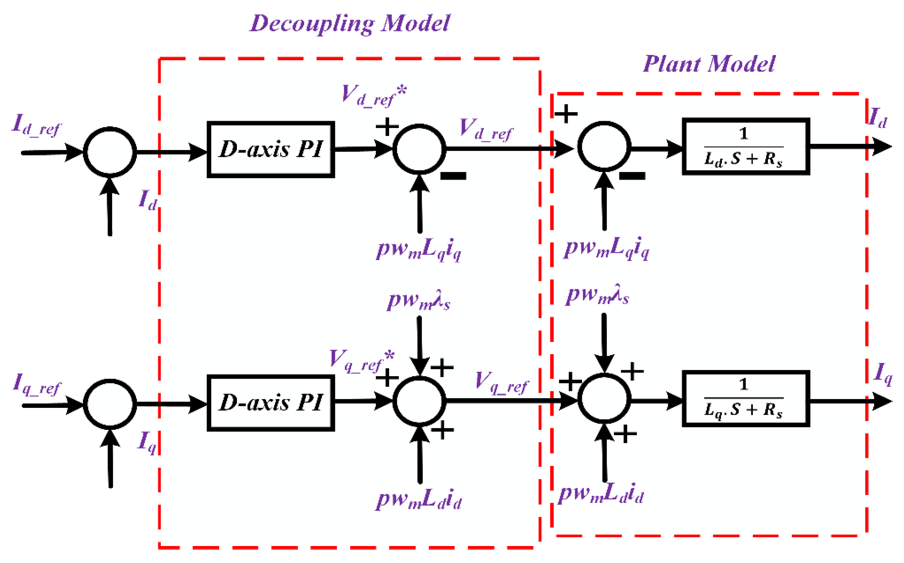
4.3. Decoupling of Torque and Flux Components
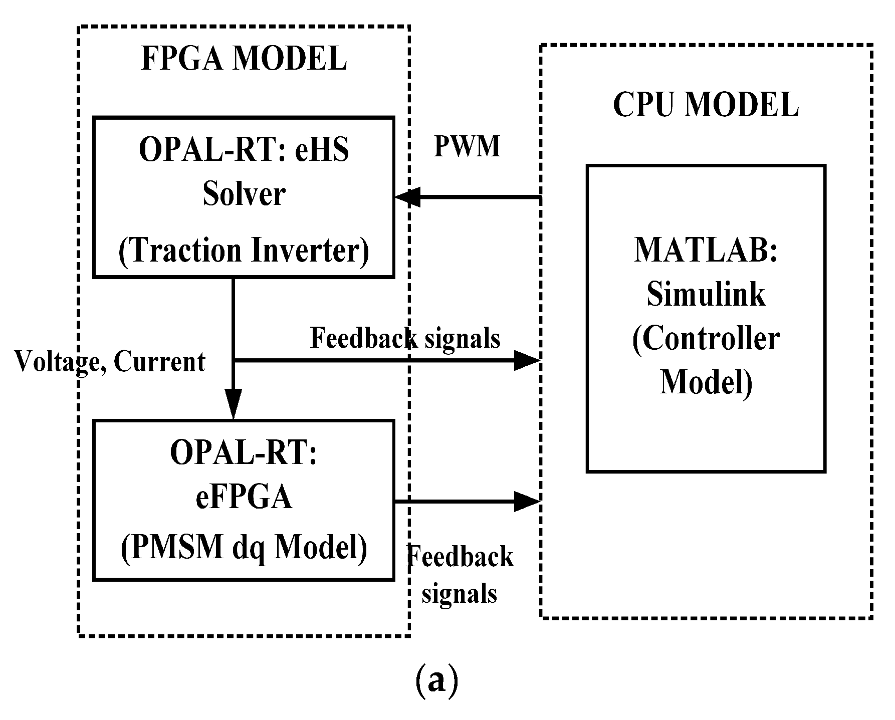
5. HIL Implementation
6. Results and Discussion
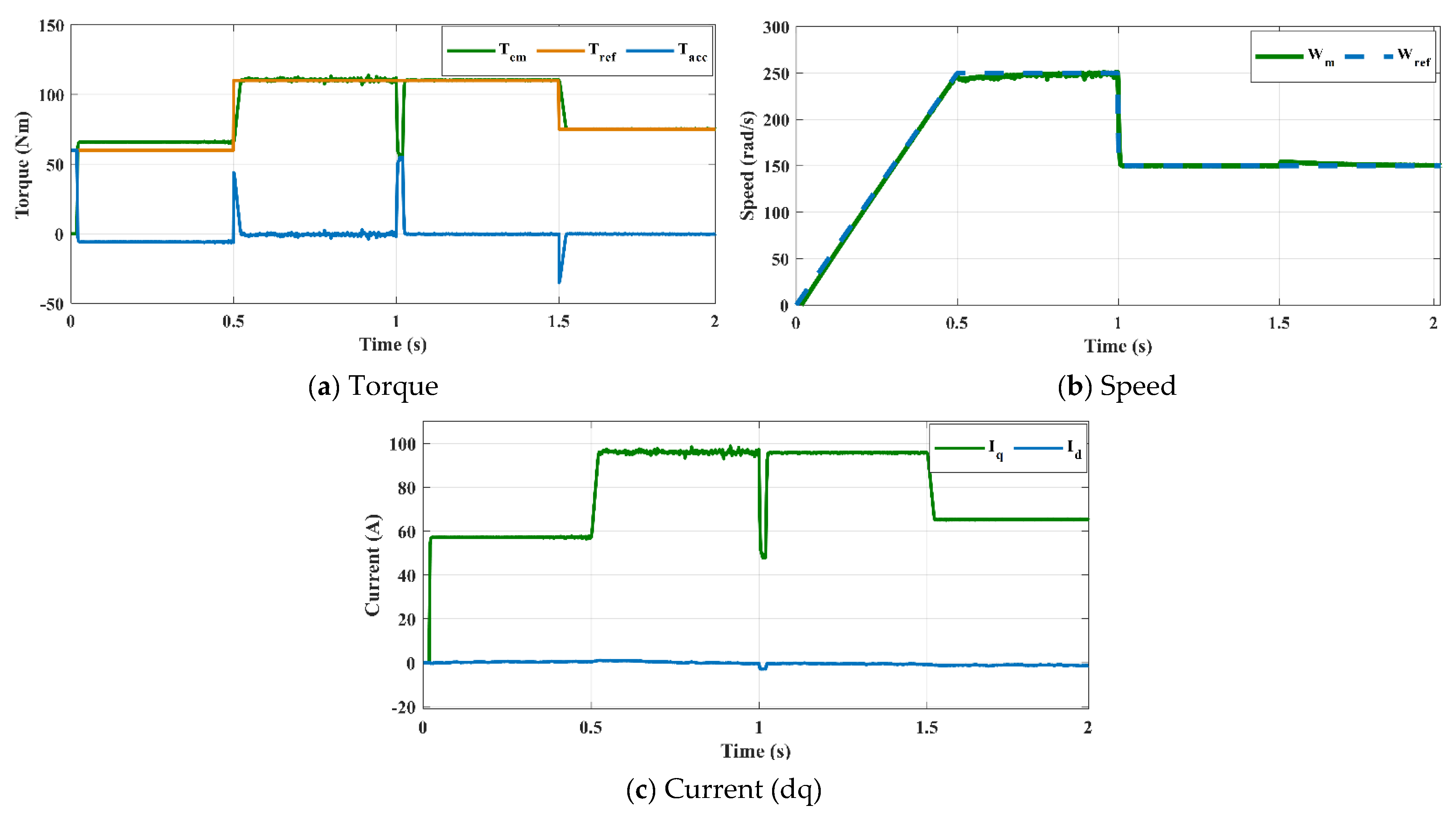
6.1. Case 1
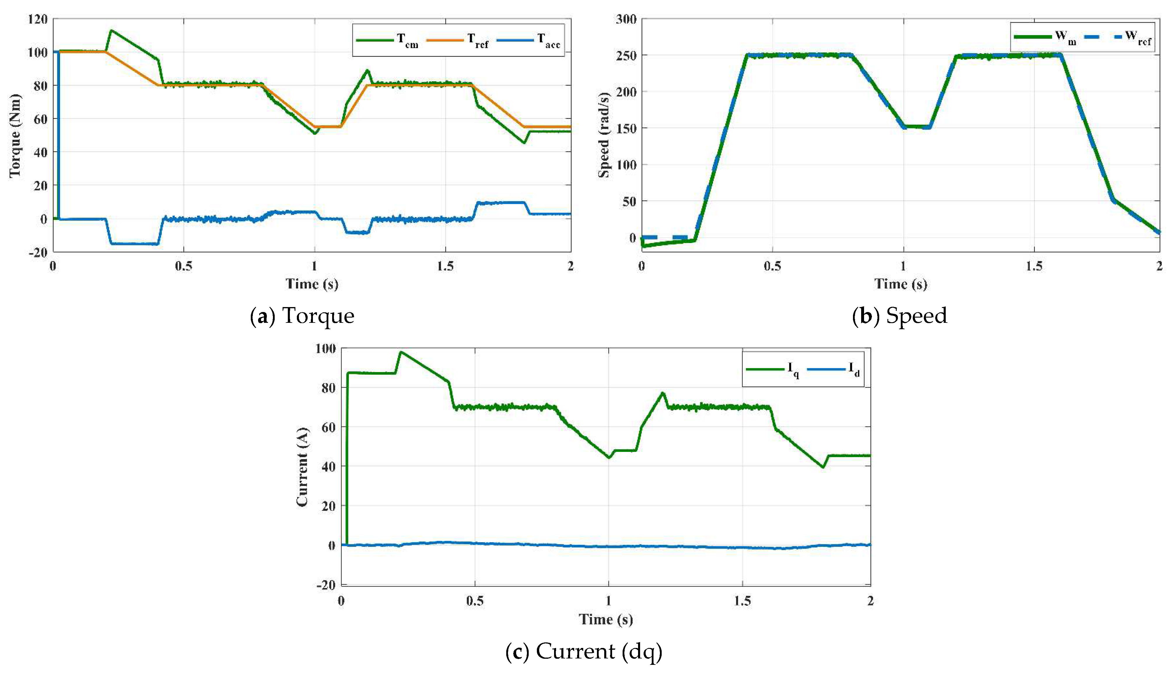
6.2. Case 2
6.3. Case 3
7. Conclusions
Author Contributions
Funding
Institutional Review Board Statement
Informed Consent Statement
Data Availability Statement
Conflicts of Interest
Nomenclature
| Rolling resistance force | |
| Aerodynamic drag force | |
| Grading resistance force | |
| Acceleration force | |
| Agriculture Implement draft force | |
| F | Soil texture adjustment parameter (dimensionless). For fine textured soil i = 1, 2 for medium and 3 for coarse textured soils. |
| A, B, C | Machine specific parameters |
| V | Operating velocity of tractor |
| W | Machine width or number of rows |
| T | Depth of tillage |
| Mass of the tractor | |
| Gravitational constant | |
| Rolling resistance coefficient | |
| Angle of gradient | |
| Air density | |
| Drag coefficient | |
| Frontal area of the tractor | |
| V | Operating velocity |
| Gross weight of the tractor | |
| Gross weight of the trailer | |
| Moment of inertia of transmission, tractor, motor, motor coupling, dynamometer and its coupling | |
| Wheel radius | |
| Gear ratio | |
| Efficiency of the transmission system | |
| Torque at wheels | |
| Shaft torque | |
| Load torque | |
| Angular velocity | |
| Voltage of d and q axis | |
| Current of d and q axis | |
| Inductance of d and q axis | |
| Electrical angular velocity | |
| Q-axis inductance | |
| Rs | Stator resistance |
| Flux linkages | |
| No of pole pairs | |
| Friction coefficient of motor, dynamometer |
References
- Mehta, C.R.; Chandel, N.S.; Jena, P.C.; Jha, A. Indian agriculture counting on farm mechanization. Agric. Mech. Asia Afr. Lat. Am. 2019, 50, 84–89. [Google Scholar]
- Fiorati, S.; Bernardini, A.; Haley, N. Electric tractor prospective. In Proceedings of the CNH Industrial, 29th Members Meeting, Hannover, Germany, 10–11 November 2019. [Google Scholar]
- Samaranayake, L.; Longo, S. Degradation control for electric vehicle machines using nonlinear model predictive control. IEEE Trans. Control Syst. Technol. 2017, 26, 89–101. [Google Scholar] [CrossRef]
- Lagnelöv, O.; Larsson, G.; Larsolle, A.; Hansson, P.A. Life cycle assessment of autonomous electric field tractors in Swedish agriculture. Sustainability 2021, 13, 11285. [Google Scholar] [CrossRef]
- Biró, N.; Kiss, P. Emission Quantification for Sustainable Heavy-Duty Transportation. Sustainability 2023, 15, 7483. [Google Scholar] [CrossRef]
- Scolaro, E.; Alberti, L.; Barater, D. Electric Drives for Hybrid Electric Agricultural Tractors. In Proceedings of the 2021 IEEE Workshop on Electrical Machines Design, Control and Diagnosis (WEMDCD), Modena, Italy, 8–9 April 2021. [Google Scholar]
- Kahveci, H.; Okumuş, H.I.; Ekici, M. Improved brushless DC motor speed controller with digital signal processor. Electron. Lett. 2014, 50, 864–866. [Google Scholar] [CrossRef]
- Amezquita-Brooks, L.; Liceaga-Castro, J.; Liceaga-Castro, E. Speed and position controllers using indirect field-oriented control:A classical control approach. IEEE Trans. Ind. Electron. 2013, 61, 1928–1943. [Google Scholar] [CrossRef]
- Kiran, K.; Das, S.; Singh, D. Model predictive field oriented speed control of brushless doubly-fed reluctance motor drive. In Proceedings of the International Conference on Power, Instrumentation, Control and Computing (PICC), Thrissur, India, 18–20 January 2018; pp. 1–6. [Google Scholar]
- Liu, T.; Chen, G.; Li, S. Application of Vector Control Technology for PMSM Used in Electric Vehicles. Open Autom. Control Syst. J. 2014, 6, 1334–1341. [Google Scholar] [CrossRef]
- Niu, L.; Yang, M.; Gui, X.; Xu, D. A comparative study of model predictive current control and FOC for PMSM. In Proceedings of the 17th International Conference on Electrical Machines and Systems (ICEMS), Hangzhou, China, 22 October 2014; pp. 3143–3147. [Google Scholar]
- Niu, F.; Wang, B.; Babel, A.S.; Li, K.; Strangas, E.G. Comparative evaluation of direct torque control strategies for permanent magnet synchronous machines. IEEE Trans. Power Electron. 2015, 31, 1408–1424. [Google Scholar] [CrossRef]
- Liu, X.; Chen, H.; Zhao, J.; Belahcen, A. Research on the performances and parameters of interior PMSM used for electric vehicles. IEEE Trans. Ind. Electron. 2016, 63, 3533–3545. [Google Scholar] [CrossRef]
- Wu, S.; Zhang, J. A robust adaptive control for permanent magnet synchronous motor subject to parameter uncertainties and input saturations. J. Electr. Eng. Technol. 2018, 13, 2125–2133. [Google Scholar]
- Lajunen, A.; Sainio, P.; Laurila, L.; Pippuri-Mäkeläinen, J.; Tammi, K. Overview of powertrain electrification and future scenarios for non-road mobile machinery. Energies 2018, 11, 1184. [Google Scholar] [CrossRef]
- Florentsev, S.; Izosimov, D.; Makarov, L.; Baida, S.; Belousov, A. Complete traction electric equipment sets of electro-mechanical drive trains for tractors. In Proceedings of the 2010 IEEE Region 8 International Conference on Computational Technologies in Electrical and Electronics Engineering (SIBIRCON), Irkutsk, Russia, 11–15 July 2010; pp. 611–616. [Google Scholar] [CrossRef]
- Troncon, D.; Alberti, L.; Mattetti, M. A Feasibility Study for Agriculture Tractors Electrification: Duty Cycles Simulation and Consumption Comparison. In Proceedings of the 2019 IEEE Transportation Electrification Conference and Expo (ITEC), Detroit, MI, USA, 19–21 June 2019. [Google Scholar] [CrossRef]
- Arjharn, W.; Koike, M.; Takigawa, T.; Yoda, A.; Hasegawa, H.; Bahalayodhin, B. Preliminary Study on the Applicability of an Electric Tractor (Part 1): Energy Consumption and Drawbar Pull Performance. J. Jpn. Soc. Agric. Mach. 2001, 63, 130–137. [Google Scholar] [CrossRef]
- Arjharn, W.; Koike, M.; Takigawa, T.; Yoda, A.; Hasegawa, H.; Bahalayodhin, B. Preliminary study on the applicability of an electric tractor (part 2). J. Jpn. Soc. Agric. Mach. 2001, 63, 92–99. [Google Scholar]
- Troncon, D.; Alberti, L. Case of study of the electrification of a tractor: Electric motor performance requirements and design. Energies 2020, 13, 2197. [Google Scholar] [CrossRef]
- Baek, S.M.; Kim, W.S.; Park, S.U.; Kim, Y.J. Analysis of Equivalent Torque of 78 kW Agricultural Tractor during Rotary Tillage. J. Korea Inst. Inf. Electron. Commun. Technol. 2019, 12, 359–365. [Google Scholar]
- Lee, D.H.; Kim, Y.J.; Choi, C.H.; Chung, S.O.; Inoue, E.; Okayasu, T. Development of a parallel hybrid system for agricultural tractors. J. Fac. Agric. Kyushu Univ. 2017, 62, 137–144. [Google Scholar] [CrossRef] [PubMed]
- Brenna, M.; Foiadelli, F.; Leone, C.; Longo, M.; Zaninelli, D. Feasibility Proposal for Heavy Duty Farm Tractor. In Proceedings of the 2018 International Conference of Electrical and Electronic Technologies for Automotive, Milan, Italy, 9–11 July 2018; pp. 1–6. [Google Scholar] [CrossRef]
- Das, A.; Jain, Y.; Agrewale, M.R.B.; Bhateshvar, Y.K.; Vora, K. Design of a Concept Electric Mini Tractor. In Proceedings of the 2019 IEEE Transportation Electrification Conference, ITEC-India, Bengaluru, India, 17–19 December 2019; pp. 10–14. [Google Scholar] [CrossRef]
- Mousazadeh, H.; Keyhani, A.; Javadi, A.; Mobli, H.; Abrinia, K.; Sharifi, A. Life-cycle assessment of a Solar Assist Plug-in Hybrid electric Tractor (SAPHT) in comparison with a conventional tractor. Energy Convers. Manag. 2011, 52, 1700–1710. [Google Scholar] [CrossRef]
- Ueka, Y.; Yamashita, J.; Sato, K.; Doi, Y. Study on the development of the electric tractor-Specifications and traveling and tilling performance of a prototype electric tractor. Eng. Agric. Environ. Food 2013, 6, 160–164. [Google Scholar] [CrossRef]
- Troncon, D.; Alberti, L.; Bolognani, S.; Bettella, F.; Gatto, A. Electrification of agricultural machinery: A feasibility evaluation. In Proceedings of the 2019 Fourteenth International Conference on Ecological Vehicles and Renewable Energies (EVER), Monte-Carlo, Monaco, 8–10 May 2019; pp. 1–7. [Google Scholar] [CrossRef]
- Matache, M.G.; Cristea, M.; Găgeanu, I.; Zapciu, A.; Tudor, E.; Carpus, E.; Popa, L.D. Small power electric tractor performance during ploughing works. Inmateh-Agric. Eng. 2020, 60, 123–128. [Google Scholar] [CrossRef]
- Yoo, I.; Lee, T.; Kim, B.; Hur, J.; Yeon, K.; Kim, G. Performance interpretation method for electrical tractor based on model-based design. In Proceedings of the 2013 International Conference on IT Convergence and Security (ICITCS), Macao, China, 16–18 December 2013; pp. 1–4. [Google Scholar] [CrossRef]
- Moreda, G.P.; Muñoz-García, M.A.; Barreiro, P. High voltage electrification of tractor and agricultural machinery—A review. Energy Convers. Manag. 2016, 115, 117–131. [Google Scholar] [CrossRef]
- Riedner, L.; Mair, C.; Zimek, M.; Brudermann, T.; Stern, T. E-mobility in agriculture: Differences in perception between experienced and non-experienced electric vehicle users. Clean Technol. Environ. Policy 2019, 21, 55–67. [Google Scholar] [CrossRef]
- Baek, S.Y.; Kim, Y.S.; Kim, W.S.; Baek, S.M.; Kim, Y.J. Development and verification of a simulation model for 120 kW class electric AWD (all-wheel-drive) tractor during driving operation. Energies 2020, 13, 2422. [Google Scholar] [CrossRef]
- Rajalakshmi, M.; Razia Sultana, W. Intelligent Hybrid Battery Management System for Electric Vehicle. In Artificial Intelligent Techniques for Electric and Hybrid Electric Vehicles; Wiley: Hoboken, NJ, USA, 2020; pp. 179–206. [Google Scholar]
- Xu, L.-Y.; Xia, X.-W.; Zhou, Z.-L.; Liu, H.-L.; Wei, M.-L. Simulation and analysis for driving system of electric tractor based on CRUISE. In Design, Manufacturing and Mechatronics, Proceedings of the 2015 International Conference on Design, Manufacturing and Mechatronics (ICDMM2015), Wuhan, China, 17–18 April 2015; World Scientific: Singapore, 2015; pp. 1367–1375. [Google Scholar] [CrossRef]
- Li, G.; Hu, J.; Li, Y.; Zhu, J. An Improved Model Predictive Direct Torque Control Strategy for Reducing Harmonic Currents and Torque Ripples of Five-Phase Permanent Magnet Synchronous Motors. IEEE Trans. Ind. Electron. 2019, 66, 5820–5829. [Google Scholar] [CrossRef]
- Morales-Caporal, R.; Leal-Lopez, M.E.; de Jesus Rangel-Magdaleno, J.; Sandre-Hernandez, O.; Cruz-Vega, I. Direct Torque Control of a PMSM-Drive for Electric Vehicle Applications. In Proceedings of the 2018 International Conference on Electronics, Communications and Computers (CONIELECOMP), Cholula, Mexico, 21–23 February 2018; Volume 2018, pp. 232–237. [Google Scholar]
- Shinohara, A.; Inoue, Y.; Morimoto, S.; Sanada, M. Maximum Torque Per Ampere Control in Stator Flux Linkage Synchronous Frame for DTC-Based PMSM Drives without Using q-Axis Inductance. IEEE Trans. Ind. Appl. 2017, 53, 3663–3671. [Google Scholar] [CrossRef]
- Abassi, M.; Khlaief, A.; Saadaoui, O.; Chaari, A.; Boussak, M. Performance Analysis of FOC and DTC for PMSM Drives Using SVPWM Technique. In Proceedings of the 2015 16th International Conference on Sciences and Techniques of Automatic Control and Computer Engineering (STA), Monastir, Tunisia, 21–23 December 2016; pp. 228–233. [Google Scholar]
- Gade, C.R.; Sultana, W.R. Battery Electric Tractor Powertrain Component Sizing with Respect to Energy Consumption, Driving Patterns and Performance Evaluation Using Traction Motor. Distrib. Gener. Altern. Energy J. 2023, 38, 789–816. [Google Scholar] [CrossRef]
- Nagar, H.; Bisaria, S.; Dalei, A.; Reddy, G.C.; Sultana, W.R.; Chitra, A. Powertrain Sizing and Performance Evaluation for Battery Electric Vehicle Using Model Based Design. In Proceedings of the 2021 Innovations in Power and Advanced Computing Technologies (i-PACT), Kuala Lumpur, Malaysia, 27–29 November 2021. [Google Scholar]
- Qin, J.; Du, J. Minimum-learning-parameter-based adaptive finite-time trajectory tracking event-triggered control for underactuated surface vessels with parametric uncertainties. Ocean. Eng. 2023, 271, 113634. [Google Scholar] [CrossRef]
- Qin, J.; Du, J.; Li, J. Adaptive finite-time trajectory tracking event-triggered control scheme for underactuated surface vessels subject to input saturation. IEEE Trans. Intell. Transp. Syst. 2023, 24, 8809–8819. [Google Scholar] [CrossRef]
- Murali, A.; Wahab, R.S.; Gade, C.S.R.; Annamalai, C.; Subramaniam, U. Assessing Finite Control Set Model Predictive Speed Controlled PMSM Performance for Deployment in Electric Vehicles. World Electr. Veh. J. 2021, 12, 41. [Google Scholar] [CrossRef]
- American Society of Agricultural and Biological Engineers. ASAE D497.7 MAR2011 Agricultural Machinery Management Data; American Society of Agricultural and Biological Engineers: St. Joseph, MI, USA, 2011; p. 9. [Google Scholar]
- Gade, C.R.; Wahab, R.S. Control of Permanent Magnet Synchronous Motor Using MPC–MTPA Control for Deployment in Electric Tractor. Sustainability 2022, 14, 12428. [Google Scholar] [CrossRef]
- Saleh, S.A.; Ozkop, E.; Nahid-Mobarakeh, B.; Rubaai, A.; Muttaqi, K.M.; Pradhan, S. Survivability-based protection for three phase permanent magnet synchronous motor drives. In Proceedings of the 2022 IEEE Industry Applications Society Annual Meeting (IAS), Detroit, MI, USA, 9–14 October 2022. [Google Scholar]
- Cendoya, M.; Solsona, J.; Toccaceli, G.; Valla, M.I. Algorithm for rotor position and speed estimation in permanent magnet ac motors. Int. J. Electron. 2002, 89, 717–727. [Google Scholar] [CrossRef]
- Bai, H.; Yu, B.; Gu, W. Research on Position Sensorless Control of RDT Motor Based on Improved SMO with Continuous Hyperbolic Tangent Function and Improved Feedforward PLL. J. Mar. Sci. Eng. 2023, 11, 642. [Google Scholar] [CrossRef]
- Lu, E.; Li, W.; Yang, X.; Liu, Y. Simulation Method of Load Characteristics of High-power PMSM Drive System. J. Phys. Conf. Ser. 2020, 1678, 012077. [Google Scholar] [CrossRef]
- Kozłowski, M.; Czerepicki, A. Quick Electrical Drive Selection Method for Bus Retrofitting. Sustainability 2023, 15, 10484. [Google Scholar] [CrossRef]
- Sultana, W.R.; Sahoo, S.K.; Karthikeyan, S.P.; Reddy, P.V.; Reddy, G.T.R.; Kiran, K.S.; Raglend, I.J. Comparative analysis of model predictive control and PWM control techniques for VSI. In Proceedings of the 2014 International Conference on Control, Instrumentation, Communication and Computational Technologies (ICCICCT), Kanyakumari, India, 10–11 July 2014; pp. 1495–1499. [Google Scholar] [CrossRef]
- Şahin, M.E.; Okumuş, H.İ. Comparison of different controllers and stability analysis for photovoltaic powered buck-boost DC-DC converter. Electr. Power Compon. Syst. 2018, 46, 149–161. [Google Scholar] [CrossRef]
- Dong, C.S.T.; Le, H.H.; Vo, H.H. Field oriented controlled permanent magnet synchronous motor drive for an electric vehicle. Int. J. Power Electron. Drive Syst. (IJPEDS) 2023, 14, 1374–1381. [Google Scholar] [CrossRef]


| Width/Units | A | B | C | F1 | F2 | F3 | |
|---|---|---|---|---|---|---|---|
| Field Cultivator | tools | 46 | 2.8 | 0 | 1 | 0.85 | 0.65 |
| Row crop planter | tools | 500 | 0 | 0 | 1 | 1 | 1 |
| Sweep Plough | m | 390 | 19 | 0 | 1 | 0.85 | 0.65 |
| Disc Harrow | m | 309 | 16 | 0 | 1 | 0.88 | 0.78 |
| Mould Board Plough | m | 652 | 0 | 5.1 | 1 | 0.75 | 0.45 |
| Parameter | Value (Unit) |
|---|---|
| Stator resistance | 0.05 ohm |
| Inductance | 0.635 mH |
| Rated power | 24 kW |
| Rated Torque (Maximum) | 111 Nm (126) |
| Speed | 290 rad/s |
| Flux linkages | 0.192 |
| pole pairs | 4 |
| Inertia | 0.011 kg-m2 |
Disclaimer/Publisher’s Note: The statements, opinions and data contained in all publications are solely those of the individual author(s) and contributor(s) and not of MDPI and/or the editor(s). MDPI and/or the editor(s) disclaim responsibility for any injury to people or property resulting from any ideas, methods, instructions or products referred to in the content. |
© 2023 by the authors. Licensee MDPI, Basel, Switzerland. This article is an open access article distributed under the terms and conditions of the Creative Commons Attribution (CC BY) license (https://creativecommons.org/licenses/by/4.0/).
Share and Cite
Gade, C.R.; Wahab, R.S. Conceptual Framework for Modelling of an Electric Tractor and Its Performance Analysis Using a Permanent Magnet Synchronous Motor. Sustainability 2023, 15, 14391. https://doi.org/10.3390/su151914391
Gade CR, Wahab RS. Conceptual Framework for Modelling of an Electric Tractor and Its Performance Analysis Using a Permanent Magnet Synchronous Motor. Sustainability. 2023; 15(19):14391. https://doi.org/10.3390/su151914391
Chicago/Turabian StyleGade, Chandrasekhar Reddy, and Razia Sultana Wahab. 2023. "Conceptual Framework for Modelling of an Electric Tractor and Its Performance Analysis Using a Permanent Magnet Synchronous Motor" Sustainability 15, no. 19: 14391. https://doi.org/10.3390/su151914391
APA StyleGade, C. R., & Wahab, R. S. (2023). Conceptual Framework for Modelling of an Electric Tractor and Its Performance Analysis Using a Permanent Magnet Synchronous Motor. Sustainability, 15(19), 14391. https://doi.org/10.3390/su151914391