Fuzzy K-Means and Principal Component Analysis for Classifying Soil Properties for Efficient Farm Management and Maintaining Soil Health

Abstract

Soil health indicators can guide soil management-related decisions for sustainable agriculture. Principle component (PC) analysis and the fuzzy k-means technique, also known as continuous classification, are useful for designing site-specific management strategies for varying soil properties within a contiguous area. The objective of this study was to identify appropriate soil health indicators as well as to create contiguous areas for precision management of a large diverse farm from measured soil properties. From the farm, which is sited on Armijo–Harkey soil, 286 loose and intact samples were obtained, representing a depth of 15 cm from the soil surface. Statistical analysis showed that several data were log-normally distributed. PCA analysis showed that the first three PCs explained 73% of the variation with PC1, consisting of factors related to the soil’s physical condition; PC2, containing factors related to chemical properties; and PC3, including factors related to macro- and micro-porosities. Minimizing the fuzziness performance index (FPI) and modified partition entropy (MPE) delineated four management classes. The membership class maps showed that the contrasting management strategies could be developed for the four management zones to achieve yield goals while conserving scarce surface water for irrigation, increasing water use efficiency, and decreasing nitrate leaching in arid and semi-arid irrigated farmlands.

1. Introduction

Soil health, previously known as soil quality, is the ability of a soil to perform normal functions, including water transport, retention, nutrient recycling, and organic carbon protection, among others [1]. Soil health assessment is useful to make useful management decisions to maintain or improve the quality and productivity of agriculture farms. The assessment usually involves measuring a series of soil chemical, physical, and microbial properties. Land use and management practices strongly influence soil health indicators [2]. Some of the major challenges of soil health assessment and management in arid areas are associated with the amount, intensity, and frequency of rainfall; land use management, including deep tillage and fallowing; and the amount and quality of irrigation water [3]. All these factors could exacerbate the variability of soil health indicators at farm scale. Understanding the spatial variability distribution of the properties of soil is required for the site-specific management of individual fields. Soil-forming factors contribute to the variability of individual soil properties as well as management-related factors (e.g., soil salinity). The coefficient of variation (CV) can be used to classify soil property variability, e.g., least (CV < 15%), moderate (15 < CV> 35%), and highest (CV > 35%) [4,5]. Precision agriculture considers the spatial variability of soil properties and makes management decisions for the sustainable utilization of resources, protecting the environment, and maintaining or increasing yield.

Several arid and semi-arid regions around the world, including southwestern states in the U.S., are predicted to become much drier in the future [6,7]. In New Mexico, the average annual precipitation is only about 230 mm, while the potential evaporation is high. New Mexico agriculture consumes about 79% of the total available water. New Mexico is also currently facing continued drought, and the surface water availability for irrigation has seen a large decline [7,8]. There is a need to manage water more carefully by decreasing losses, increasing water use efficiency, and improving on-farm management. Some of these could be achieved by examining several physical and chemical parameters together rather than looking at each property individually.

Principle component analysis (PCA) can group several measured soil properties into few components, and those can be interpreted as soil health indicators [2]. Although these groups are constructed using a statistical analysis tool, the groups often represent specific soil functions. The variations in the properties within each component could be monitored over time, and those can be used to determine if soil health is improving, staying stable, or degrading [5,9].

The current manuscript divides a field in which soil properties have low variability into zones for efficient farm management [10,11,12]. The objective of this research is to create contiguous homogenous zones that form the basis for the optimal utilization of inputs such as seeds, fertilizers, or irrigation. Classes are defined from the available data that have a significant impact on crop yield, such as the soil’s physical properties, i.e., texture and bulk density, which affect soil’s water-holding capacity [13,14]. Each class consists of a set of measured data that are analyzed statistically and grouped together based on their variability class. The final output is the delineation of unique contiguous zones for which a similar management plan can be carried out. Moreover, there are several different approaches that can be used to obtain management zones. The fuzzy k-means procedure has been used successfully to identify zones for efficient management [15,16]. Similar attributes are grouped into distinct classes or ‘clusters’ based on the properties measured at each individual location [10,17,18,19]. Each class function is dependent on the interrelationships between physical and chemical properties within that class [11]. Hence, the identification and mapping of soil classes is important for the application of precision agriculture technologies.

Fuzzy k-means analysis creates different classes, and an individual soil property belongs fully, partially, or not at all to a certain class [20]. Fuzzy k-means classification is also called continuous classification [21] and provides more precise information about the variability and character of the data than is provided by the discrete classes [22]. The continuous classification for each location produces a class membership for available data points. To determine the dominance of a class, a confusion index (CI) is used. For no confusion, the CI is equal to zero; however, when the dominance of any class is not evident, CI is equal to one. Spatial correlations of memberships have an inverse relationship with CI zones. Shukla et al. [22] used fuzzy k-means with extra grades and created contiguous homogenous zones in a field using different soil physical and chemical properties. Rong-Jiang et al. [23] used fuzzy k-means analysis to identify the variability of soil properties that limit yield. Many studies have reported the usefulness of continuous classification [18,19,22]. Therefore, this study was conducted using measured soil properties to identify soil health indicators using PCA and the fuzzy k-means technique to create contiguous zones for site-specific management of an agricultural farm.

2. Materials and Methods

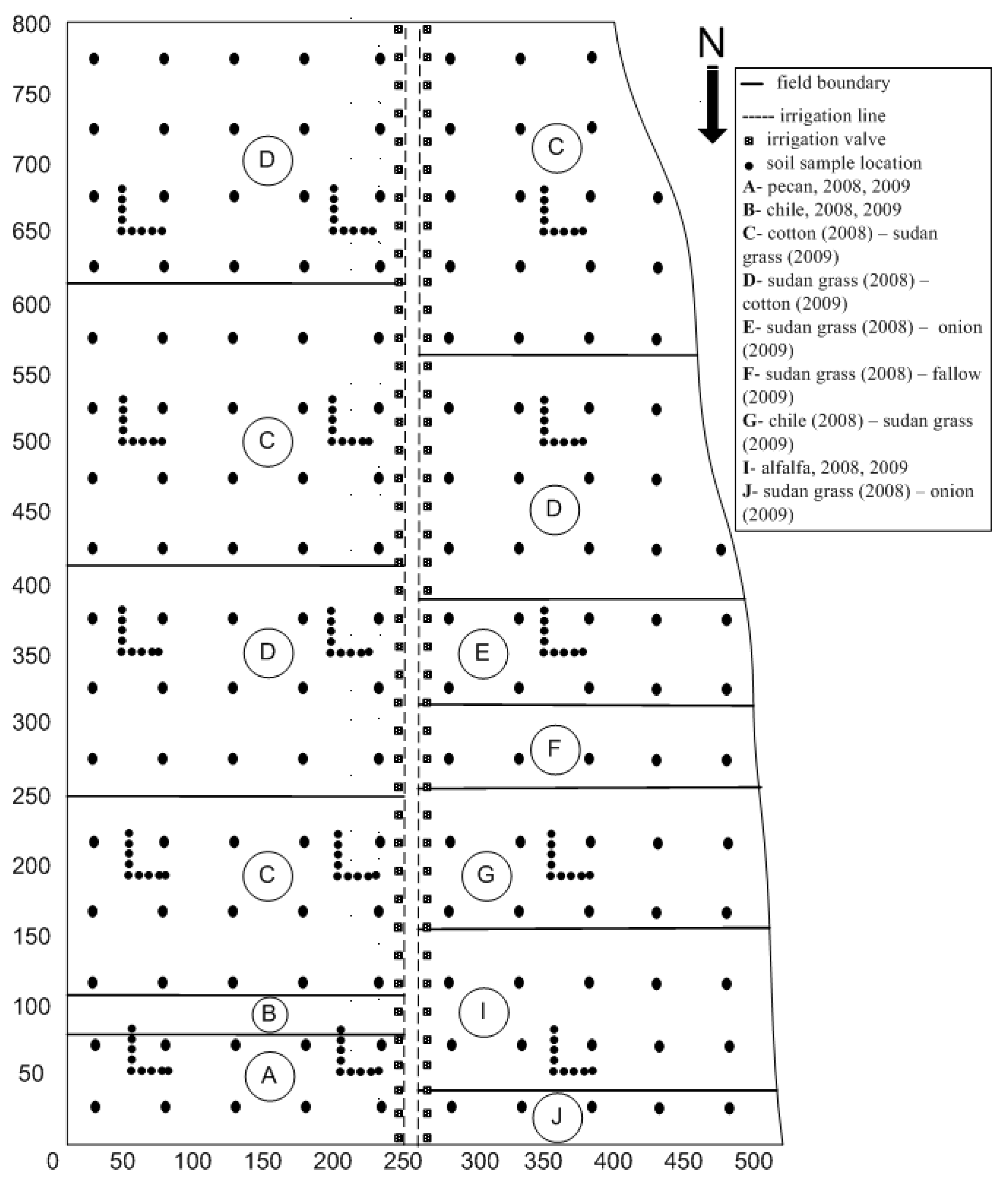
2.1. Experimental Site

This study utilized the data collected from a 40 ha agricultural farm known as the Leyendecker Plant Science Research Center (LPSRC). The LPSRC is located near Las Cruces (32°11.46′ N and 106°44.30′ W), New Mexico [24]. The Rio Grande River flows from north to south about 85 m away on the west side of the farm. There is a drainage ditch near the east boundary of the farm (15 m). The farm is planted with alfalfa (Medicago sativa L.), chile (Capsicum annuum L.), cotton (Gossypium spp.), onion (Allium cepa L.), pecan (Carya illinoinensis (Wangenh.) K. Koch), and Sudan grass (Sorghum Sudanense (Piper.) Stapf.). Armijo (fine-silty, mixed, calcareous, thermic-typic Torrifluvents) and Harkey (coarse-silty, mixed, calcareous, thermic-typic Torrifluvents) series are the dominant soils.

For the study area, the average annual precipitation recorded was 25.4 cm and the average annual temperature was 17.7 °C. The groundwater table depth from the soil surface was recorded every minute using a U20 data logger (hobo; onset computer corporation, Bourne, MA, USA). The data showed that water table depth fluctuated between 2.5 and 4 m. The study site had 12 different units, and for the past 9 years since 2009, the same crop rotation was practiced in each of the units (Figure 1). The Sudan grass was the main rotational crop in each unit. At the end of the growing season, the cash crop was replaced with Sudan grass after the harvest, but no rotation was needed for alfalfa and pecan. The farm was irrigated with groundwater unless surface water was available. Except the Sudan grass, each crop was fertilized with urea (46-0-0) or urea ammonium nitrate (URAN) (46-0-0). The rate of application was 200 kg N ha⁻¹ for crops. For every crop except Sudan grass, a broadcast application of triple super phosphate (0-45-0) was made in February. The preplant application was conducted at a rate of 200 kg P₂O₅ ha⁻¹ in the study area.

2.2. Soil Sampling and Analysis

For the purpose of collecting core and loose soil samples, the experimental area was divided into 16 transects parallel to the x-axis. During November 2008, 286 loose and core soil samples were obtained at the depth of 0-15 cm. Additionally, during November 2009, 286 loose soil samples were obtained from the same locations (Figure 1). The area was divided into a grid of 50x50 m, and 151 samples were collected at the center of each grid. To account for the short-range variability, another 135 samples were obtained at 2, 5, 10, and 15 m intervals on some locations indicated in Figure 1. A global positioning system (GPS) determined the longitude and latitude of each sampling location.

All loose soil samples were initially air-dried for 72 h after the larger sized clods were broken by hand. Once the samples were dry, they were ground using a wooden mallet and ground samples passing through a 2 mm sieve were retained in plastic Ziploc bags. About 51 g of dried sieved sample (<2 mm) was used to determine the particle size analysis using the hydrometer method [25].

The soil from both ends of the cylindrical cores of known weight and diameter was removed. The soil cores were subsequently weighed. The soil bulk density, BD, was determined on intact cores [26]. After the soil BD was determined, two layers of cheesecloth were placed at one end of each core and tied with a rubber band. The undisturbed cores were then left in a tray filled with water for 48 h, and they were saturated via capillary rise at room temperature. The saturated hydraulic conductivity, Ks, for each soil core was measured using the constant head method [27]. Subsequently, θ at six different suctions ψ_m (−33, −100, −300, −500, −1000 and −1500 kPa) were determined on the same intact cores using the pressure plate apparatus [28]. A 3- and a 5-bar presoaked ceramic plate was used to determine the soil water retention curve. The suction was raised slowly from 0 kPa to −33 kPa, and equilibrium at any suction was maintained for 24 h. After that, the soil cores were removed from the extractor and were weighed, and the same procedure was repeated for the remaining suctions. The θ at each ψ_m increment was calculated on the weight basis. The value of θ at −1500 kPa was designated as the permanent wilting point (WP) and the value of θ at −33 kPa was classified as the field capacity (FC). Plant available water content, AWC, was obtained by subtracting θ at FC and θ at WP. The volume of transport pores (VTP) were of size > 50 μm, the volume of storage pores (VSP) was between 0.5 and 50 μm, and the volume of residual pores (VRP) was <0.5 μm.

2.3. Descriptive Statistics and Normality

Using the SAS program, statistical analyses of soil properties were conducted for 2008 and 2009, separately [29]. All measured data for all the soil physical and chemical properties were first checked for normality using the Shapiro–Wilk (SW) test. The SW test showed that all the measured soil data were significantly skewed (p < 0.05), and most soil properties were not normally distributed. The measured properties were transformed using a natural logarithm and some of the properties became near normal. There were some high measured Ks values. These high values were mostly from areas under coarse textured soils, and made data distribution non-normal. However, these values were retained. The transformed data were used to determine the descriptive statistics, including the mean, range, maximum and minimum, coefficient of variation, skewness, kurtosis, standard deviation (SD), and standard error (SE). The spatial variability analysis of soil physical and chemical properties has already been published by Sharma et al. [24].

2.4. Principal Component Analysis

The principal component analysis used a correlation matrix, in which all data were standardized, using Statistical Analysis System [29]. PCs with eigenvalues > 1 were subjected to varimax rotation to maximize correlations among components.

2.5. Fuzzy-K Means Analysis

The fuzzy k-means technique provided the continuous maps [30]. The fitting parameter, alpha (α), was determined as the relative ratio of extragrades to intragrades. Several values of fuzzy exponents starting from 1 to 5 were run and a value of 1.3 was selected [31]. The class membership map for each soil property was obtained using continuous classification. Care was taken to ensure that equal area of membership was assigned to each class. The optimum numbers of classes were obtained by minimizing the fuzziness performance index (FPI) and modified partition entropy (MPE). The clear distribution of the memberships of each class was obtained by determining the confusion index (CI) as follows:

$$CI=1-({\mu }_{\max i}-{\mu }_{(\max -1)i})$$

where μ_maxi is the membership value of the class with the maximum μ_max at site i, and μ_(max−1)i is the second-largest membership value at the same site.

3. Results and Discussion

3.1. Data Variability

Most measured soil parameters were non-normally distributed. The skewness for sand, silt, BD, Ks, ranged from +0.38 to +3.12. However, for clay, FC, WP, and AWC, the skewness was negative and ranged from −0.29 to −1.04 (Sharma et al. [24]). The Ks data were highly skewed with a skewness of 3.12 and a range of 72.22 cm/d. This was primarily due to the large soil variability from west to east. The fields along the northwest to southwest corners were closer to the river and were dominated by coarse textured sandy soils from the soil surface. High Ks values were related to the greater macro porosities associated with coarse-textured soils. The EC and chloride showed small positive skewness (<1.2), but the skewness for NO₃-N was high (1.71). This was consistent with other studies that reported no salinity issues in the experimental site [24]. The higher skewness for NO₃-N was associated with the variability of soil types across the experimental domain from east to west. In some studies, non-normal data were transformed to obtain near-normal distributions of the data. Several different methods were reported for data transformation, including natural logarithm, square root, and squared, among others [32,33]. Many previous studies did not attempt to transform the non-normal data [34]. However, we transformed the data using a natural logarithm. The transformed data were more normally distributed than the original data. For example, log-transformation of the sand content data resulted in the data following a normal distribution. However, the Shapiro–Wilk test also showed that some data remained non-normal even after the log transformation. Other researchers have concurred with our results and reported smaller decreases in kurtosis compared to the skewness after the transformation [17,32].

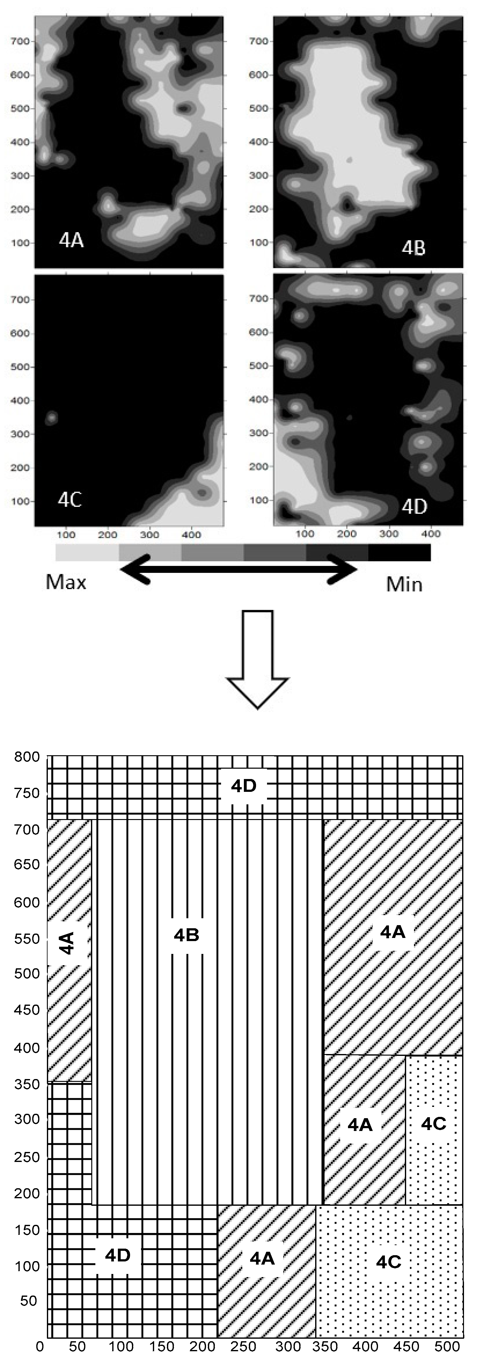
3.2. Principal Component Analysis

The first three PCs explained 73% of variability and each of them have an eigenvalue greater than 1.6 (

Table 1. The principal components (PC), eigenvalues and the individual and cumulative variance explained.

PC	Eigenvalue	Difference	Proportion	Cumulative
1	5.78	3.62	0.44	0.44
2	2.17	0.56	0.17	0.61
3	1.60	0.68	0.12	0.73

). The first PC explained about 44% of the variance, the second 17% and the third about 12%. The magnitude of eigenvalue was used to explain the correlation between a PC and a soil property, and a soil property was assigned to a PC for which its eigenvalue was the highest. A soil property achieves a higher preference when it explains a higher proportion of variance with a higher communality estimate than the other does. Thus, volume of residual pores (VRP) was the least important soil property and field capacity (FC) water content was the most important soil property. The major soil variables that contributed to PC1 were bulk density (r = −0.94), and FC and wilting point (WP) water contents (r > 0.94). Other soil variables that contributed to PC1 were clay content (r = 0.92) and hydraulic conductivity (Ks; r = −0.85). The major contributing soil variables for PC2 were electrical conductivity (EC; r = 0.95), nitrate–nitrogen (r = 0.91) and chloride (Cl; r = 0.53). The major contributing soil variables for PC3 were available water content (AWC; r = 0.73), volume of transport pores (VTP; r = −0.63), and volume of storage (VSP) pores and volume of residual pores (VRP; r > 0.63 (

Table 2. Proportion of the variance obtained with varimax rotation and communality estimates (CE) for soil property variables of the three retained principal components (PCs).

Variable	PC1	PC2	PC3	CE
Sand	−0.88	0.00	−0.12	0.78
Clay	0.92	0.08	0.03	0.86
BD	−0.94	−0.06	−0.04	0.88
KS	−0.85	−0.01	−0.17	0.76
FC	0.94	0.06	0.19	0.93
WP	0.95	0.05	−0.06	0.91
AWC	0.19	0.03	0.73	0.57
EC	0.06	0.95	−0.04	0.91
NO3-N	−0.08	0.91	−0.02	0.83
Cl	0.47	0.53	−0.09	0.51
VTP	−0.48	0.03	−0.63	0.63
VSP	0.09	−0.15	0.68	0.50
VRP	−0.29	0.03	0.63	0.48

where BD is soil bulk density, Ks is soil hydraulic conductivity, FC and WP are field capacity and wilting point water contents, respectively, AWC is available water content, EC is electrical conductivity, Cl is chloride, VTP, VST and VRP are volumes of transport, storage, and residual pores, respectively.

). Based on the communality estimates, FC water content was the most dominant factor, followed by wilting point water content, soil EC, BD, and soil NO₃-N content. Soil BD usually has a strong correlation with soil moisture contents of the soil. Since soil organic carbon content (SOC) was less than 1% in the experimental farm, it was not included in the soil health assessment. SOC is generally reported as an important soil health indicator in mid-western US states [35]. Our results indicate that for the study area, located in the arid southwest, the dominant soil health parameters were part of the PC1 and PC2. To maintain or increase soil health and productivity, soil moisture status as well as soil NO₃-N should be monitored regularly and maintained at sufficient levels to not cause water or nutritional imbalance.

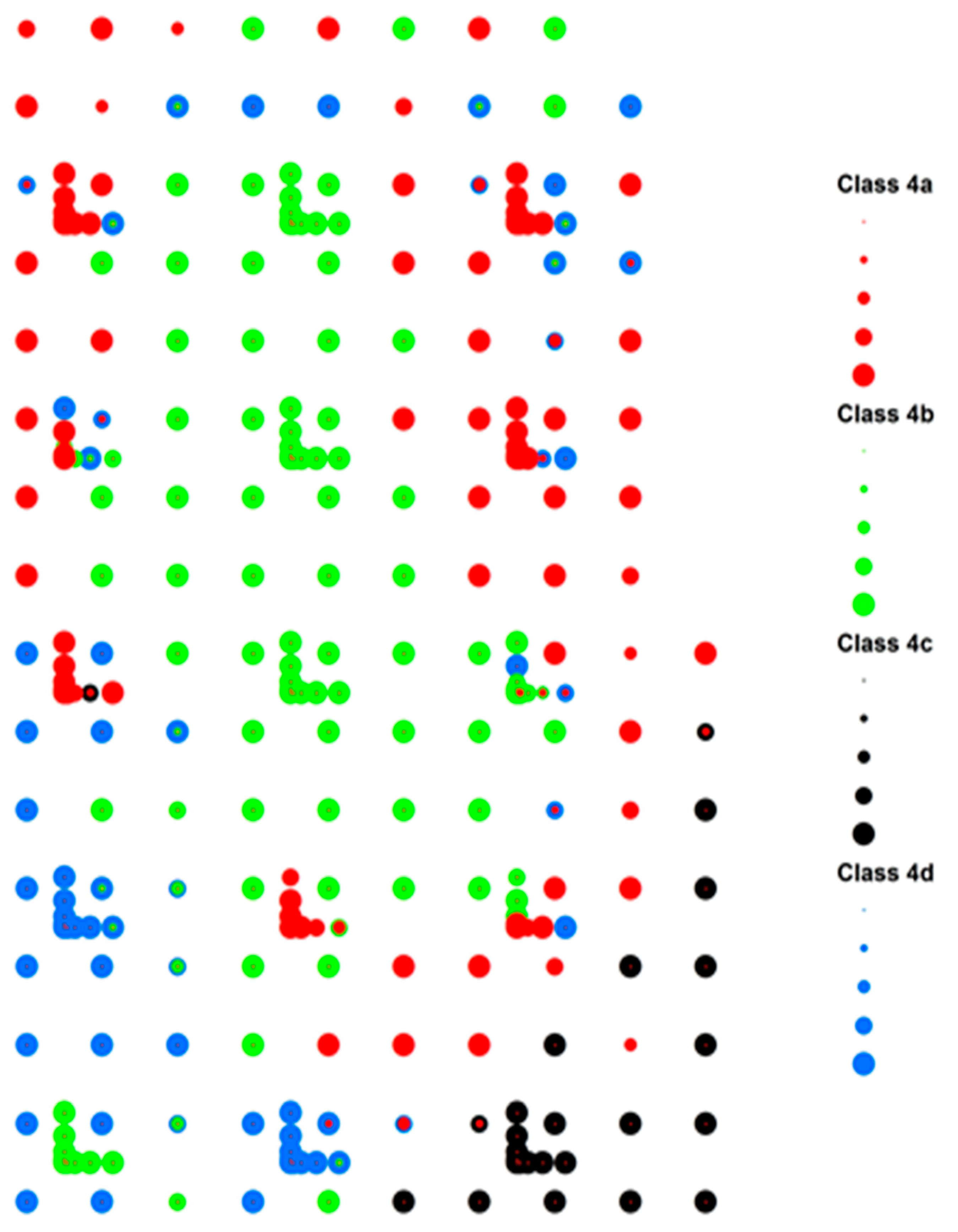
3.3. Fuzzy K-Means Clustering

Fuzzy k-means classification was used to delineate distinct classes consisting of measured soil properties. Figure 2 presents FPI and MPE with respect to the number of classes. It is evident from the figure that the slope of the curve was initially steep and by the time it reached the class value of four; it became gradual to asymptotic. Therefore, four classes were deemed sufficient to divide the whole dataset. Using similar selection criteria, other researchers have also reported management zones for their study [14,22,36].

The soil attributes for the four classes (

Table 3. The four identified classes and the mean values of some soil properties using continuous classification.

Parameter	Sand %	Silt %	Clay %	BD g/cm3	Ks cm/d	WP %	FC %
4a	36.94	25.41	37.65	1.31	7.06	20.90	33.10
4b	26.39	23.16	50.46	1.25	4.22	28.67	40.03
4c	53.95	27.20	18.85	1.45	49.26	12.43	23.02
4d	24.22	32.73	43.04	1.27	5.58	24.17	37.25

BD = bulk density; Ks = saturated hydraulic conductivity; WP = wilting point; FC = field capacity.

) showed differences among the physical properties of the classes that could have an important impact on the soil behavior. Class 4a had the medium soil texture, bulk density, saturated hydraulic conductivity, water content at field capacity, and wilting point. Class 4b experienced the highest clay content and lowest BD, and Ks, whereas the water content at WP and FC was also highest among all four classes. Class 4c had the highest sand content, BD and Ks. The water content at WP and FC was lowest for class 4c among all the four classes. Class 4d had the lowest sand content and medium BD and Ks. The water content was also medium at WP and FC. As the differences between the classes were distinctive, the fuzzy k-means clustering technique could delineate four clusters (classes) within the entire experimental farm. Similar analysis for soil fertility attributes have also been presented by other researchers [22].

There were instances in which a single data point participated in more than one class. The degree to which a single point integrated with different classes is represented by the confusion index [37]. Membership would be relatively small if the confusion index is large for any single class. ArcGIS software was used to delineate the four classes on the map of the experimental area. The distribution of the four classes within the experimental area is shown in Figure 3. Class 4a was mostly clustered near the west border but also had an influence near the east border of the study area. Class 4b was prominent mainly in the middle of the study area. Class 4c was strongly clustered only in the northwest corner of the experimental area. Class 4d was found mainly along the east, west and some parts of the north border of the study area.

The class that has the highest membership is designated as the dominant class at each site and is shown in Figure 4. The size of the mark indicates the degree of dominance of the membership in that class. The CI and the membership have an inverse relationship; and generally, sites with high CI have low membership. The drawn maps in Figure 4 grouped soils with similar physical properties. Maps based upon CI also delineated the transition zones in the study area. Thus, four distinct field management zones were delineated, and contrasting management strategies were proposed to achieve efficient water use, environmental, and certain yield goals. For example, class 4a, 4b, and 4d had fine-textured soils compared to class 4c that had coarse-textured soils. Therefore, switching irrigation to a drip system from the current furrow irrigation could be a better option for efficient water management in the northwest corner of the study area. Water application at lower amounts and higher frequency in this part of the field would improve the crop water use efficiency. Using similar logic, water application rates and frequency for irrigating other fields could be based on the measured soil properties within each of the four management classes. Zone 4c has mostly sandy soil and therefore the existing furrow and flood irrigation system is not conducive for maintaining yield as well as preventing nitrate leaching [38]. Chen et al. [36] noted similar observations and reported increases in yield under variable irrigation management. Similar contiguous management zones were identified based on several soil physical, hydraulic and chemical properties by Shukla et al. [22] for an experimental farm in Austria; Yao et al. [39] for a farm in the Jiangsu province, China; and Zhu et al. [40] for the northern Appalachian Ridge, USA. Delineation of management zones is an effective way to increase on-farm efficiencies and it can provide a good tradeoff between crop yield and water applied. Continuous classification could guide precision agriculture management for sustainable utilization of available resources in large farms.

4. Conclusions

Measuring soil physical and chemical properties is important when making decisions about regular on-farm management. In water-scarce areas, knowledge of the variability of soil physical properties, such as saturated hydraulic conductivity, is important for water conservation and increasing water use efficiencies. The PCA analysis showed that the first three PCs explained about 73% of the variability of soil physical, hydraulic, and chemical properties. Soil moisture status and soil nitrogen were identified as the dominant soil health parameters. Soil bulk density was also found to be an important variable that was closely related to soil moisture status. Delineating different zones of management within a large farmland would optimize irrigation volumes, conserve water, and increase yields. This study demonstrated that continuous classification provided better management of the farm with regard to water and nutrient management and yields.

References

1. Karlen, D.L.; Ditzler, C.A.; Andrews, S.S. Soil quality: Why and how? Geoderma 2003, 114, 145–156. [Google Scholar] [CrossRef]
2. van Es, H.M.; Karlen, D.L. Reanalysis Validates Soil Health Indicator Sensitivity and Correlation with Long-term Crop Yields. Soil Sci. Soc. Am. J. 2019, 83, 721–732. [Google Scholar] [CrossRef]
3. Shukla, M.K. New Journal: Soil Health (Editorial). 1.1. 2021. Available online: https://oaepublish.com/sh/article/view/4442 (accessed on 5 May 2022).
4. Wilding, L.P. Spatial variability: Its documentation, accommodation, and implication to soil surveys. In Soil Spatial Variability; Nielsen, D.R., Bouma, J., Eds.; Pudoc: Wageningen, The Netherlands, 1985; pp. 166–194. [Google Scholar]
5. Shukla, M.K.; Lal, R.; Ebinger, M. Principal component analysis for predicting biomass and corn yield under different land uses. Soil Sci. 2004, 169, 215–224. [Google Scholar] [CrossRef]
6. Setter, T.; Waters, I. Review of prospects for germplasm improvement for waterlogging tolerance in wheat, barley and oats. Plant Soil 2003, 253, 1–34. [Google Scholar] [CrossRef]
7. Cayan, D.R.; Das, T.; Pierce, D.W.; Barnett, T.P.; Tyree, M.; Gershunov, A. Future dryness in the southwest US and the hydrology of the early 21st century drought. Proc. Natl. Acad. Sci. USA 2010, 107, 21271–21276. [Google Scholar] [CrossRef]
8. Williams, A.P.; Cook, B.I.; Smerdon, J.E. Rapid intensification of emerging southwestern North American mega-drought in 2020–2021. Nat. Clim. Chang. 2021, 12, 232–234. [Google Scholar] [CrossRef]
9. Brejda, J.I.; Moorman, T.B.; Karlen, D.L.; Dao, T.H. Identification of regional soil quality factors and indicators. I. Central and southern high plains. Soil Sci. Soc. Am. J. 2000, 64, 2115–2124. [Google Scholar] [CrossRef]
10. Lark, R.M. Forming spatially coherent regions by classification of multi-variate data: An example from the analysis of maps of crop yield. Int. J. Geogr. Inf. Sci. 1998, 12, 83–98. [Google Scholar] [CrossRef]
11. Guastaferro, F.; Castrignano, A.; De Benedetto, D.; Sollitto, D.; Troccoli, A.; Cafarelli, B. A comparison of different algorithms for the delineation of management zones. Precision Agric. 2010, 11, 600–620. [Google Scholar] [CrossRef]
12. Farid, H.U.; Bakhsh, A.; Ahmad, N.; Ahmad, A.; Mahmood-Khan, Z. Delineating site-specific management zones for precision agriculture. J. Agric. Sci. 2016, 154, 273–286. [Google Scholar] [CrossRef]
13. Gessler, P.E.; Chadwick, O.A.; Chamran, F.; Althouse, L.; Holmes, K. Modeling Soil-Landscape and Ecosystem Properties Using Terrain Attributes. Soil Sci. Soc. Am. J. 2000, 64, 2046–2056. [Google Scholar] [CrossRef]
14. Davatgar, N.; Neishabouri, M.R.; Sepaskhah, A.R. Delineation of site specific nutrient management zones for a paddy cultivated area based on soil fertility using fuzzy clustering. Geoderma 2012, 173–174, 111–118. [Google Scholar] [CrossRef]
15. Bansod, B.S.; Pandey, O.P. An application of PCA and fuzzy C-means to delineate management zones and variability analysis of soil. Eurasian Soil Sci. 2013, 46, 556–564. [Google Scholar] [CrossRef]
16. Hedley, C. The role of precision agriculture for improved nutrient management on farms. J. Sci. Food Agric. 2015, 95, 12–19. [Google Scholar] [CrossRef] [PubMed]
17. Trangmar, B.; Yost, R.S.; Uehara, C. Application of geostatistics to spatial studies of soil properties. Adv. Agron. 1985, 38, 45–94. [Google Scholar]
18. Valente, D.S.M.; Queiroz, D.M.; Pinto, F.A.C.; Santos, N.T.; Santos, F.L. Definition of management zones in coffee production fields based on apparent soil electrical conductivity. Sci. Agric. 2012, 69, 173–179. [Google Scholar] [CrossRef]
19. Li, Y.; Shi, Z.; Wu, H.-X.; Li, F.; Li, H.-Y. Definition of Management Zones for Enhancing Cultivated Land Conservation Using Combined Spatial Data. Environ. Manag. 2013, 52, 792–806. [Google Scholar] [CrossRef]
20. Bezdek, J.C. Pattern Recognition with Fuzzy Objective Function Algorithm; Plenum Press: New York, NY, USA, 1981. [Google Scholar]
21. McBratney, A.B.; De Gruijter, J.J. A continuum approach to soil classification by modified fuzzy k-means with extragrades. J. Soil Sci. 1992, 43, 159–175. [Google Scholar] [CrossRef]
22. Shukla, M.K.; Slater, B.K.; Lal, R.; Cepuder, P. Spatial variability of soil properties and potential management classification of a chernozemic field in lower Austria. Soil Sci. 2004, 169, 852–860. [Google Scholar] [CrossRef]
23. Termin, D.; Linker, R.; Baram, S.; Raveh, E.; Ohana-Levi, N.; Paz-Kagan, T. Dynamic delineation of management zones for site-specific nitrogen fertilization in a citrus orchard. Precision Agric. 2023, 24, 1570–1592. Available online: https://link.springer.com/article/10.1007/s11119-023-10008-w (accessed on 5 May 2022). [CrossRef]
24. Nyéki, A.; Daróczy, B.; Kerepesi, C.; Neményi, M.; Kovács, A.J. Spatial Variability of Soil Properties and Its Effect on Maize Yields within Field—A Case Study in Hungary. Agronomy 2022, 12, 395. [Google Scholar] [CrossRef]
25. Gee, G.W.; Bauder, J.W. Particle-size analysis. In Methods of Soil Analysis. Part 1, 2nd ed.; Agron. Monogr. No. 9.; Klute, A., Ed.; ASA and SSSA: Madison, WI, USA, 1986; pp. 383–411. [Google Scholar]
26. Blake, G.R.; Hartge, K.H. Bulk density. In Methods of Soil Analysis. Part 1, 2nd ed.; Agron. Monogr. No. 9.; Klute, A., Ed.; ASA and SSSA: Madison, WI, USA, 1986; pp. 363–376. [Google Scholar]
27. Klute, A.; Dirkson, C. Hydraulic conductivity and diffusivity: Laboratory methods. In Methods of Soil Analysis. Part 1, 2nd ed.; Agron. Monogr. No. 9.; Klute, A., Ed.; ASA and SSSA: Madison, WI, USA, 1986; pp. 687–734. [Google Scholar]
28. Klute, A. Water retention: Laboratory methods. In Methods of Soil Analysis. Part 1, 2nd ed.; Agron. Monogr. No. 9.; Klute, A., Ed.; ASA and SSSA: Madison, WI, USA, 1986; pp. 635–662. [Google Scholar]
29. SAS Institute. SAS/STAT User’s Guide. Version 6, 4th ed.; SAS Institute: Cary, NC, USA, 1989; Volume 1–2. [Google Scholar]
30. Minasny, B.; McBratney, A.B. Fuzzy K-Mean with Extragrades, Version 3; Australian Centre for Precision Agriculture, The University of Sidney: Sidney, Australia, 2006. [Google Scholar]
31. McBratney, A.; Moore, A. Application of fuzzy sets to climatic classification. Agric. For. Meteorol. 1985, 35, 165–185. [Google Scholar] [CrossRef]
32. Cambardella, C.A.; Moorman, T.B.; Novak, J.M.; Parkin, T.B.; Karlen, D.L.; Turco, R.F.; Konopka, A.E. Field-Scale Variability of Soil Properties in Central Iowa Soils. Soil Sci. Soc. Am. J. 1994, 58, 1501–1511. [Google Scholar] [CrossRef]
33. Schenatto, K.; de Souza, E.G.; Bazzi, C.L.; Gavioli, A.; Betzek, N.M.; Beneduzzi, H.M. Normalization of data for delineating management zones. Comput. Electron. Agric. 2017, 143, 238–248. [Google Scholar] [CrossRef]
34. Özgöz, E. Long Term Conventional Tillage Effect on Spatial Variability of Some Soil Physical Properties. J. Sustain. Agric. 2009, 33, 142–160. [Google Scholar] [CrossRef]
35. Shukla, M.K.; Lal, R.; Ebinger, M. Determining soil quality indicators by factor analysis. Soil Till. Res. 2006, 87, 194–204. [Google Scholar] [CrossRef]
36. Chen, S.; Wang, S.; Shukla, M.K.; Wu, D.; Guo, X.; Li, D.; Du, T. Delineation of management zones and optimization of irrigation scheduling to improve irrigation water productivity and revenue in a farmland of Northwest China. Precis. Agric. 2019, 21, 655–677. [Google Scholar] [CrossRef]
37. Burrough, P.; van Gaans, P.; Hootsmans, R. Continuous classification in soil survey: Spatial correlation, confusion and boundaries. Geoderma 1997, 77, 115–135. [Google Scholar] [CrossRef]
38. Stites, W.; Kraft, G. Nitrate and Chloride Loading to Groundwater from an Irrigated North-Central U.S. Sand-Plain Vegetable Field. J. Environ. Qual. 2001, 30, 1176–1184. [Google Scholar] [CrossRef] [PubMed]
39. Yao, R.-J.; Yang, J.-S.; Zhang, T.-J.; Gao, P.; Wang, X.-P.; Hong, L.-Z.; Wang, M.-W. Determination of site-specific management zones using soil physico-chemical properties and crop yields in coastal reclaimed farmland. Geoderma 2014, 232–234, 381–393. [Google Scholar] [CrossRef]
40. Zhu, Q.; Lin, H.; Doolittle, J. Functional soil mapping for site-specific soil moisture and crop yield management. Geoderma 2013, 200–201, 45–54. [Google Scholar] [CrossRef]
Figure 1. Sample design and location of samples in the study site, adopted from Sharma et al. [24].
Sustainability 15 13144 g001
Figure 2. Fuzziness performance index (FPI) and modified position entropy (MPE) for continuous classification.
Sustainability 15 13144 g002
Figure 3. Spatial distribution of class membership for the four identified classes. The approximate rectangular shapes can provide easier management of the entire farm.
Sustainability 15 13144 g003
Figure 4. The spatial distribution of the dominating class map. The map shows the class with the highest membership value and the degree of membership within the dominant class.
Sustainability 15 13144 g004