Exploring the Spatiotemporal Dynamics of CO₂ Emissions through a Combination of Nighttime Light and MODIS NDVI Data

Abstract

Climate change caused by CO₂ emissions is posing a huge challenge to human survival, and it is crucial to precisely understand the spatial and temporal patterns and driving forces of CO₂ emissions in real time. However, the available CO₂ emission data are usually converted from fossil fuel combustion, which cannot capture spatial differences. Nighttime light (NTL) data can reveal human activities in detail and constitute the shortage of statistical data. Although NTL can be used as an indirect representation of CO₂ emissions, NTL data have limited utility. Therefore, it is necessary to develop a model that can capture spatiotemporal variations in CO₂ emissions at a fine scale. In this paper, we used the nighttime light and the Moderate Resolution Imaging Spectroradiometer (MODIS) normalized difference vegetation index (NDVI), and proposed a normalized urban index based on combination variables (NUI-CV) to improve estimated CO₂ emissions. Based on this index, we used the Theil–Sen and Mann–Kendall trend analysis, standard deviational ellipse, and a spatial economics model to explore the spatial and temporal dynamics and influencing factors of CO₂ emissions over the period of 2000–2020. The experimental results indicate the following: (1) NUI-CV is more suitable than NTL for estimating the CO₂ emissions with a 6% increase in average $R^2$. (2) The center of China’s CO₂ emissions lies in the eastern regions and is gradually moving west. (3) Changes in industrial structure can strongly influence changes in CO₂ emissions, the tertiary sector playing an important role in carbon reduction.

1. Introduction

Global warming, glacial melting, and ocean level rise caused by climate change have created great threats to human survival and development [1,2,3]. If global temperatures continue to rise, it is possible that more extreme weather events will occur. How to deal with climate change has become a thorny issue for scholars from all over the world [4,5]. It has been widely accepted that CO₂ emissions are a major cause of climate change and that fossil fuel combustion is the main contributor to CO₂ emissions [6,7]. Curbing energy-related CO₂ emissions is a necessary path to achieve carbon neutrality and is the key to mitigating the human climate crisis [8]. As its economy grows, China’s demand for fossil fuels is also increasing. At present, China has the highest level of CO₂ emissions in the world [9,10,11]. In the context of climate change, China has formulated many measures to reduce CO₂ emissions. In 2015, the Chinese government showed its determination to save energy and reduce emissions. It pledged to achieve a 60–65% reduction in CO₂ emissions intensity by 2030 compared to 2005 [12]. Therefore, an accurate and comprehensive understanding of the spatiotemporal distribution and driving forces of CO₂ emissions is a prerequisite for implementing precise emission reduction strategies [13,14,15].

In different parts of a city, CO₂ emissions may have different spatial dynamics, but statistical data can only show the overall development of a city and cannot reveal the urban internal landscapes [16]. Therefore, how to investigate CO₂ emissions at a fine-scale has become an important topic of concern to many scholars. It has been pointed out that nighttime light data (e.g., the Defense Meteorological Satellite Program’s Operational Linescan System [DMSP-OLS] and the Visible Infrared Imaging Radiometer Suite Day/Night Band [VIIRS-DNB]) can describe socio-economic phenomena related to human activities [17]. These data are widely used in studies on urbanization [18,19,20], poverty analysis [21,22], impervious surface extraction [23,24,25], environmental variations [26,27,28], population spatialization [29,30], electric power consumption [31,32] and economic analysis [33,34,35]. Since nighttime light is highly correlated with human activity, and CO₂ emissions are an inevitable product of human activities, a connection can be made between nighttime light with CO₂ emissions [36,37]. Doll et al. found a high correlation between CO₂ emissions and DMSP-OLS nighttime light data, and mapped the distribution of CO₂ emissions at a global scale [38]. Ghosh et al. introduced population distribution data to model CO₂ emissions from people in areas with more or less nighttime light [39]. However, their method was relatively simple and the DMSP-OLS data have limitations in estimating CO₂ emissions [40,41]. The spatial resolution of DMSP-OLS is about 1000 m, and it cannot distinguish pixels with values larger than 63. All values larger than 63 are recorded as 63, and the phenomenon is the saturation effect [42,43]. Due to the saturation effect and coarse spatial resolution of DMSP-OLS, it fails to reflect the differences in core urban areas in detail [32,44]. Although many scholars have proposed various correction methods for this problem, these methods may provide quite different results [45,46,47]. VIIRS-DNB not only has a higher spatial resolution, but also has a longer detection range without saturation effects [48]. Since the release of VIIRS-DNB data, the higher spatial resolution and longer detection range have motivated scholars to perform higher resolution studies [49,50]. Shi et al. demonstrated that VIIRS-DNB is a powerful indicator for modeling socioeconomic phenomena [51].

Although nighttime light data can study the CO₂ emissions in cities, there are still some shortcomings in using nighttime light data alone [12,24,52,53]. More and more scholars are introducing vegetation cover data (e.g., normalized difference vegetation index [NDVI]) into their studies [23,54]. Experiments have shown that this combination provides good results in impervious surface area (ISA) mapping. However, few surveys use this method to estimate CO₂ emissions. Based on the existing studies, some scholars have studied the changes in CO₂ emissions at different scales, but they only summarized CO₂ emissions of different administrative units, and the trend of CO₂ emissions on pixels is still unclear [7,16,55]. Although some scholars have simply analyzed the change of CO₂ emissions, significant analysis of trends in changes is still lacking [10,47]. Additionally, the analysis of the spatial and temporal dynamic patterns and the influencing factors related to CO₂ emissions is not comprehensive [56]. Therefore, it is necessary to conduct an in-depth and systematic analysis of the influencing factors related to CO₂ emissions [57,58,59].

In this study, a new combination index was proposed to improve the estimation accuracy of CO₂ emissions. We then aimed to explore the trends and significance in CO₂ emissions at the pixel scale. Furthermore, we investigated the spatial and temporal dynamics of CO₂ emissions and the drivers of CO₂ emissions were discussed.

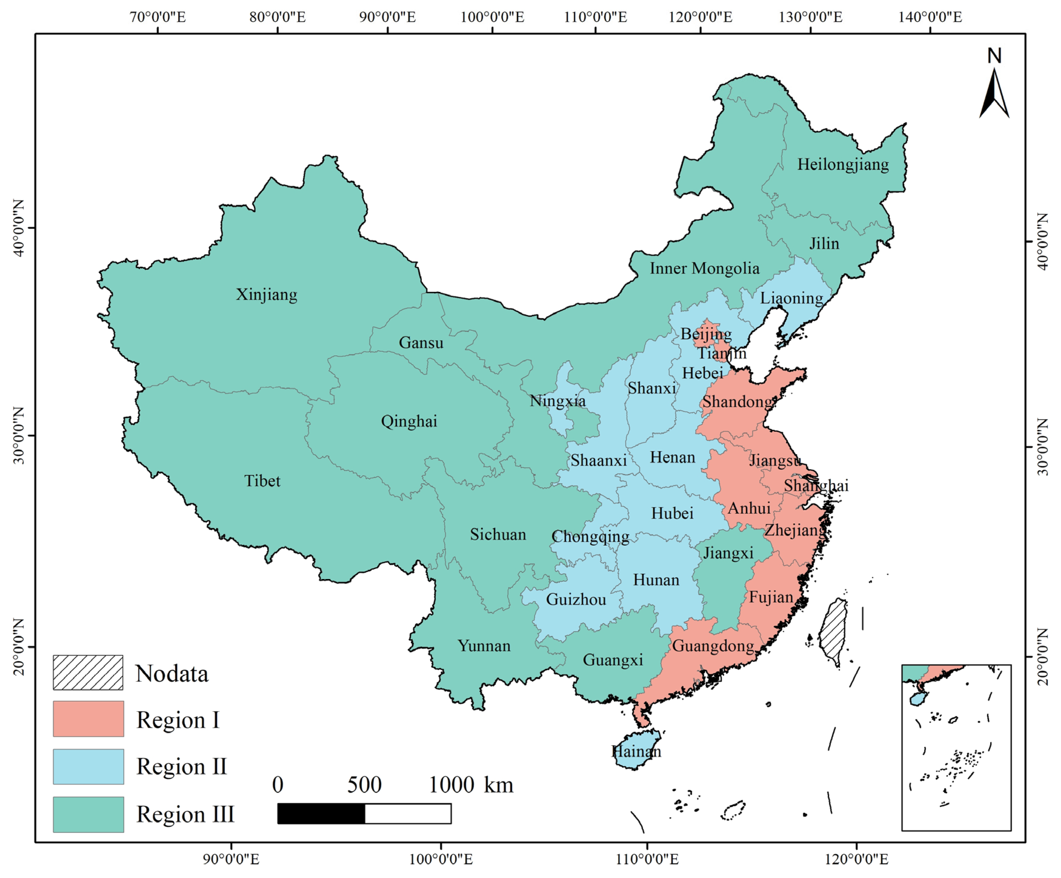
2. Study Area and Datasets

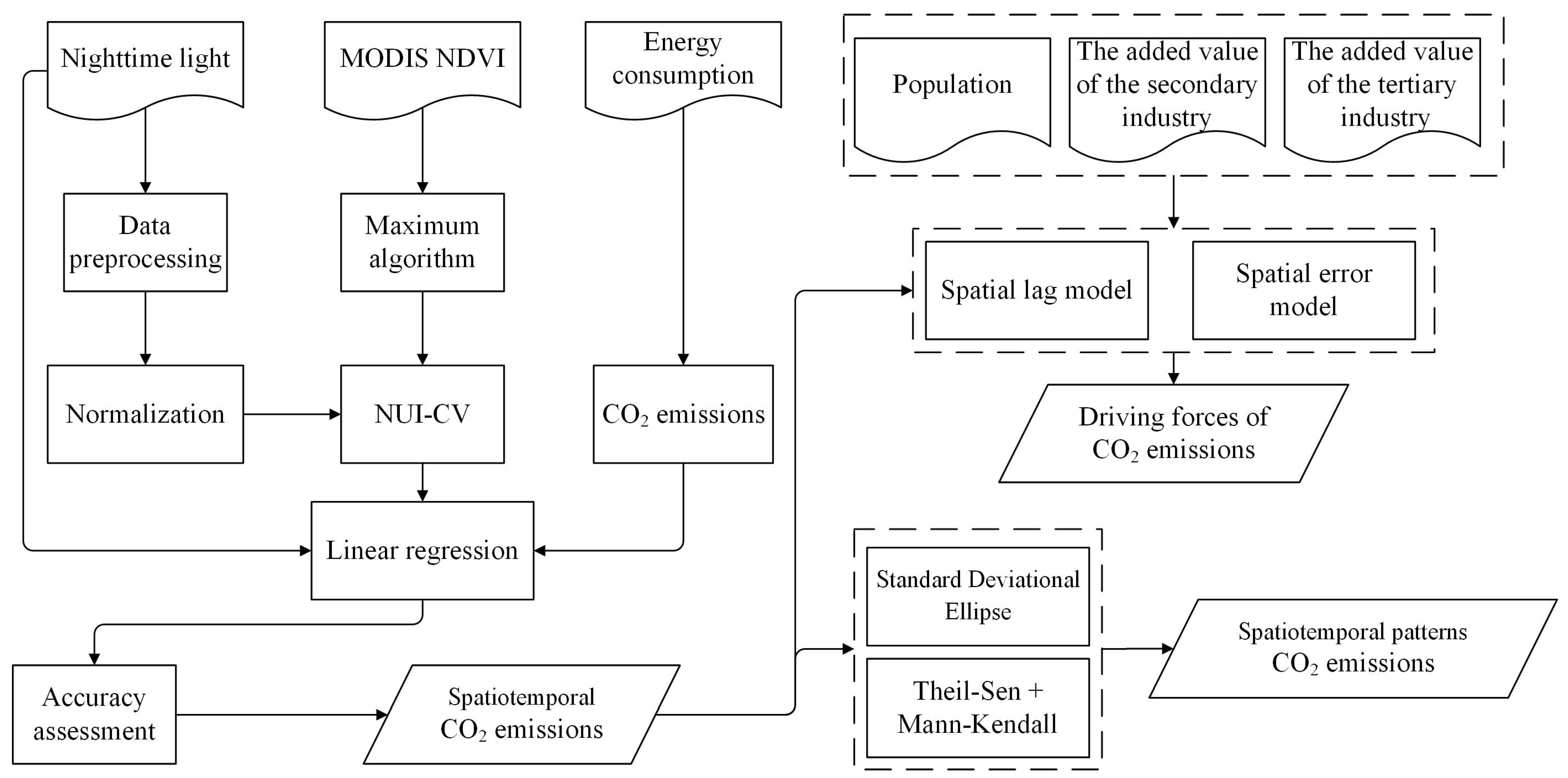
Mainland China is the main area under examination in this paper and we divided the study area into three major regions based on the research by Guo et al. [53]. The detailed region division results are shown in Figure 1. The datasets used in this study are nighttime light imageries, MODIS NDVI product, energy consumption statistics, socioeconomic data and administrative boundaries.

Nighttime light data from 2000 to 2020 were used, referring to the method proposed by Chen et al. [60], and the original dataset of 2000–2012 was taken from the enhanced vegetation index-adjusted NTL index (EANTLI) dataset [61]. By integrating DMSP-OLS and enhanced vegetation index (EVI) data, EANTLI can reduce the saturation effect of DMSP-OLS and enhance image information:

$$EANTLI=\frac{1+({NTL}_{nor }-EVI)}{1-({NTL}_{nor}-EVI)}\times NTL$$

(1)

where ${NTL}_{nor}$ denotes the normalized DMSP-OLS, $EVI$ is an annual data of EVI, and $NTL$ is the original nighttime light brightness.

Monthly VIIRS-DNB data after 2013 were used to produce an annual median VIIRS-DNB dataset to obtain more reliable annual data. Then, the annual VIIRS-DNB products were treated with reference to Shi et al. [51], who proposed an auto-encoder model with convolutional neural networks (CNN) to transform EANTLI data into VIIRS-DNB-like data. The data from 2013 and 2012 were used as the training and testing sets, respectively. This dataset can describe the dynamic changes of socio-economic characteristics accurately over a long time period with a resolution of 15 arc-second (~500 m). Although NTL can be used as an indirect representation of CO₂ emissions, NTL data have limited utility. Therefore, it is necessary to introduce additional data to capture the spatiotemporal variations in CO₂ emissions at a fine scale. Among them, vegetation cover data is regarded as a data source that can effectively supplement the nighttime light information.

MODIS NDVI (MOD13A1) data were downloaded from the Google Earth Engine platform and produced as an annual product. The energy consumptions were obtained from the China Energy Statistics Yearbook, which describes eight energy types and can be used to estimate CO₂ emissions. Statistics, such as year-end population, added value of the secondary industry (AVSI), and added value of the tertiary industry (AVTI) were downloaded from the China National Bureau of Statistics. The administrative boundary data of the country and its provinces were taken from China’s National Geomatics Centre. The details of the dataset are summarized in

Table 1. Datasets used in research.

Data	Description	Year	Source
Nighttime light (DMSP-OLS, VIIRS-DNB)	Long time series of global nighttime light data.	2000–2020	https://dataverse.harvard.edu/dataset.xhtml?persistentId=doi:10.7910/DVN/YGIVCD (accessed on 13 August 2023)
MODIS NDVI (MOD13A1)	Global 500 m spatial resolution 16-day product.	2000–2020	Google Earth Engine platform (https://code.earthengine.google.com/, accessed on 13 August 2023)
Energy consumption data	Energy statistics for 30 provinces (104 t).	2000–2020	China Energy Statistics Yearbook
Socioeconomic data	Three types of socio-economic indicators: population, AVSI, and AVTI.	2000, 2010, 2020	China National Bureau of Statistics

.

3. Methods

There were four steps in our research methods. First, we preprocessed the remote sensing data to maintain the same resolution and coordinate system. Second, CO₂ emissions were calculated from energy consumption. Third, we investigated the spatiotemporal dynamics of CO₂ emissions. Finally, the driving forces behind CO₂ emissions were discussed. The detailed process is shown in Figure 2.

3.1. Preprocessing of Remote Sensing Data

For the uniformity of projection, all remote sensing data (i.e., nighttime light and MODIS NDVI) were reprojected to the Albers Conical Equal Area projection and resampled to 500 m resolution.

In order to avoid the impacts of outliers, we set the maximum of nighttime light to 100, and all pixels with DN values greater than 100 were set to 100. The reason for setting this threshold is that most pixel values in the nighttime light imageries are less than 100 [24]. After that, the nighttime light data were normalized with Equation (2):

$${NTL}_{nor}=\frac{NTL-{NTL}_{min}}{{NTL}_{max}-{NTL}_{min}}$$

(2)

where ${NTL}_{nor}$ is the normalized nighttime light data, with a range of 0–1; and ${NTL}_{max}$ and ${NTL}_{min}$ represent the maximum and minimum pixel values, respectively.

To avoid the confusion of bare soil, water bodies, and ISA, we used the maximum value method to composite the multi-period NDVI images:

$${NDVI}_{max}=MAX\left[{NDVI}_1,{NDVI}_2,\cdots ,{NDVI}_n\right]$$

(3)

where ${NDVI}_1$, ${NDVI}_2$, …, ${NDVI}_n$ are the multitemporal MOD13A1 NDVI images.

3.2. Estimation of CO₂ Emissions

We used the formula developed by the Intergovernmental Panel on Climate Change (IPCC) to compute statistical CO₂ emissions [62]. The statistical CO₂ emissions ($SC$) can be formulated by:

$$SC={\sum }_{w=1}^W{E}_w\times {CEC}_w\times {ALC}_w$$

(4)

where $E$ represents the amount of energy consumption, $\omega$ denotes the energy types, and $CEC$ and $ALC$ are the carbon emission coefficients and the average low-order calorific values, respectively.

A new index is presented here, named the Normalized Urban Index Based on Combination Variables (NUI-CV), which combines the nighttime light (NTL) and MODIS NDVI datasets:

$$\mathrm{N}\mathrm{U}\mathrm{I}\mathrm{-}\mathrm{C}\mathrm{V}=\left(1-{NDVI}_{max}\right)\times {log}_2\left(1+\sqrt{{NTL}_{nor}}\right)$$

(5)

Since ${NDVI}_{max}$ is negatively associated with urban sprawl, $1-{NDVI}_{max}$ (ranging between 0 and 1) is positively associated with urban information. ${log}_2\left(1+\sqrt{{NTL}_{nor}}\right)$ not only smooths the extreme values of nighttime light, but also holds the value between 0–1. The information on human activities can be enhanced by integrating NTL and NDVI datasets in this way. To verify the accuracy of NUI-CV, we modeled NTL and NUI-CV, respectively, with CO₂ emissions using a linear regression model. It is because linear regression models are able to describe the relationship between different variables intuitively and are simple to implement and widely used.

3.3. Assessment of Spatiotemporal Dynamics of CO₂ Emissions

3.3.1. Analysis of CO₂ Emissions Trend

The Theil–Sen and Mann–Kendall (TS-MK) trend analysis method included Theil–Sen slope estimation and the Mann–Kendall test [63]. Theil–Sen slope estimation is generally employed to calculate the trend value, and it is insensitive to outliers in the series dataset. However, it cannot provide significance judgments and usually needs to be performed together with the Mann–Kendall test [64]. The Mann–Kendall test is a non-parametric time series trend test that provides the significance of the trend of change. TS-MK is often used in the studies related to vegetation cover and climate change. In this paper, the method is used to detect the significance of the change trend of CO₂ emissions.

The Theil–Sen slope formula is:

$$\beta =Median\left(\frac{x_j-x_i}{j-i}\right),j>i$$

(6)

where $\beta$ represents the trend degree; when $\beta$ is greater than 0 means that CO₂ emissions are increasing over time, when $\beta$ is less than 0 means that CO₂ emissions are decreasing; $x_i$ and $x_j$ represent the carbon emissions in years $i$ and $j$.

The statistical values associated with Mann–Kendall test are calculated, as shown in equation.

$$S={\sum }_{i=1}^{n-1}{\sum }_{j=i+1}^{n}sgn\left(x_j-x_i\right),sgn\left(x_j-x_i\right)=\left\{\begin{array}{cc}+1,& x_j>x_i\\ 0,\hfill & x_j=x_i\\ -1,& x_j<x_i\end{array}\right.$$

(7)

$$\mathit{Z}=\left\{\begin{array}{cc}\frac{S-1}{\sqrt{VAR\left(S\right)}},\hfill & S>0\\ 0,\hfill & S=0\\ \frac{S-1}{\sqrt{VAR\left(S\right)}},& S>0\end{array}\right.,Var\left(S\right)=\frac{n\left(n-1\right)\left(2n+5\right)}{18}$$

(8)

where $n$ is the time period (2000–2020), $S$ is the test statistic, $Var\left(S\right)$ is the variance of $S$, and $Z$ denotes the significance.

According to different confidence levels, $\beta$ and $Z$ are classified into different categories. The detailed categories are found in

Table 2. Categories of changes in CO₂ emission trends.

$\mathit{\beta }$	$\mathit{Z}$	Trend Category
$\beta >0$	$2.58<\left|Z\right|$	Extremely significant increase
	$1.96<\left|Z\right|\le 2.58$	Significant increase
	$1.65<\left|Z\right|\le 1.96$	Slightly significant increase
	$\left|Z\right|\le 1.96$	Not significantly increased
$\beta =0$	Any value	No change
$\beta <0$	$\left|Z\right|\le 1.96$	Not significantly decrease
	$1.65<\left|Z\right|\le 1.96$	Slightly significant decrease
	$1.96<\left|Z\right|\le 2.58$	Significant decrease
	$2.58<\left|Z\right|$	Extremely significant decrease

.

3.3.2. CO₂ Emissions Evolution Direction

Standard deviational ellipse (SDE) can describe the spatial distribution of data from multiple directions [65]. By analyzing various parameters related to SDEs, the direction and the change in the distribution trend of CO₂ emissions can be obtained [66]. The weighted mean center is the center of the spatial distribution and can be calculated using Equation (6):

$$M\left(\widehat{x},\widehat{y}\right)=\left(\frac{{\sum }_{i=1}^n{w}_i{x}_i}{{\sum }_{i=1}^n{w}_i},\frac{{\sum }_{i=1}^n{w}_i{y}_i}{{\sum }_{i=1}^n{w}_i}\right)$$

(9)

where $M\left(\widehat{x},\widehat{y}\right)$ is the weighted mean center, $x_i$ and $y_i$ are the coordinates of spatial unit $i$, $\omega$ denotes the spatial weight, and $n$ represents the sum of spatial units. The rotation angle can be described with $\tan \theta$ as follows:

$$\tan \theta =\frac{\left({\sum }_{i=1}^n{\tilde{x}}_i^2-{\sum }_{i=1}^n{\tilde{y}}_i^2\right)+\sqrt{{\left({\sum }_{i=1}^n{\tilde{x}}_i^2-{\sum }_{i=1}^n{\tilde{y}}_i^2\right)}^2+4{\left({\sum }_{i=1}^n{\tilde{x}}_i{\tilde{y}}_i\right)}^2}}{2{\sum }_{i=1}^n{\tilde{x}}_i{\tilde{y}}_i}$$

(10)

where $\theta$ is the azimuth angle of the ellipse, and ${\tilde{x}}_i$ and ${\tilde{y}}_i$ denote the deviation of the XY coordinate from the weighted mean center.

$${\delta }_x=\sqrt{\frac{{\sum }_{i=1}^n{\left(w_i{\tilde{x}}_i\cos \theta -w_i{\tilde{y}}_i\sin \theta \right)}^2}{{\sum }_{i=1}^n{w}_i^2}}$$

(11)

$${\delta }_y=\sqrt{\frac{{\sum }_{i=1}^n{\left(w_i{\tilde{x}}_i\sin \theta -w_i{\tilde{y}}_i\cos \theta \right)}^2}{{\sum }_{i=1}^n{w}_i^2}}$$

(12)

In the above equation, ${\delta }_x$ and ${\delta }_y$ are the standard deviations of the ellipse x-axis and y-axis, respectively.

3.4. Driving Force Analysis of CO₂ Emissions

In contrast to the traditional econometrics, spatial econometric models are able to adequately account for spatial dependence [67]. The first law of geography proposed by Tobler et al. highlights the existence of interactions between spatial units and provides a theoretical basis for spatial measurement [68]. To investigate how the spatial effects influence CO₂ emissions, here the spatial lag model (SLM) and spatial error model (SEM) were introduced into the experiment. The SLM represents the impact of CO₂ emissions from surrounding provinces on CO₂ emissions in a particular city [69]. The model is specified as follows:

$$Y=\rho WY+X\beta +\mu$$

(13)

where $X$ and $Y$ represent the dependent and independent variable matrices, respectively, $\rho$ denotes the spatial effect coefficient, $W$ represents the spatial matrix, $\beta$ is the parameter vector, and $\mu$ denotes the random error vector, satisfying $\mu ~N\left(0,{\sigma }^2\right)$.

The SEM assumes that the spatial error term is correlated with the spatial totality [70]. The error of an individual will affect other individuals with spatial effects:

$$Y=X\beta +\epsilon$$

(14)

$$\epsilon =\lambda W\epsilon +\mu$$

(15)

where $\lambda$ represents the coefficient of spatial error term and $\epsilon$ is the error term of spatial auto-correction.

Previous studies have indicated that differences in population and industrial structure are major contributors to CO₂ emissions [12,53]. However, few scholars constructed SLM and SEM to investigate their relationship with CO₂ emissions.

4. Results and Discussion

4.1. Comparative Analysis of Variables and Models

Figure 3 illustrates the detailed information of a different dataset at the same position. Compared with NTL, NUI-CV can enrich the detailed information within the city. To compare the reliability of CO₂ emissions, we employed a linear regression model to validate the estimated CO₂ from NTL and NUI-CV, respectively.

Table 3. $R^2$ comparison of experimental results.

Year	NTL	NUI-CV	Year	NTL	NUI-CV
2000	0.5794	0.6461	2011	0.725	0.7718
2001	0.5336	0.6312	2012	0.6069	0.7035
2002	0.7525	0.7547	2013	0.7519	0.8251
2003	0.7706	0.7772	2014	0.7436	0.7907
2004	0.7643	0.7848	2015	0.6644	0.7716
2005	0.7096	0.7373	2016	0.6698	0.7554
2006	0.6908	0.7429	2017	0.679	0.7719
2007	0.763	0.7887	2018	0.6328	0.7259
2008	0.7148	0.7481	2019	0.616	0.7117
2009	0.5992	0.7075	2020	0.5829	0.6754
2010	0.7211	0.7666	Average	0.6796	0.7423

showed that the average $R^2$ of NUI-CV (0.74) was significantly higher than that of NTL (0.68). As a conclusion, NUI-CV is more suitable than NTL for estimating CO₂ emissions.

4.2. Spatiotemporal CO₂ Emissions Dynamics

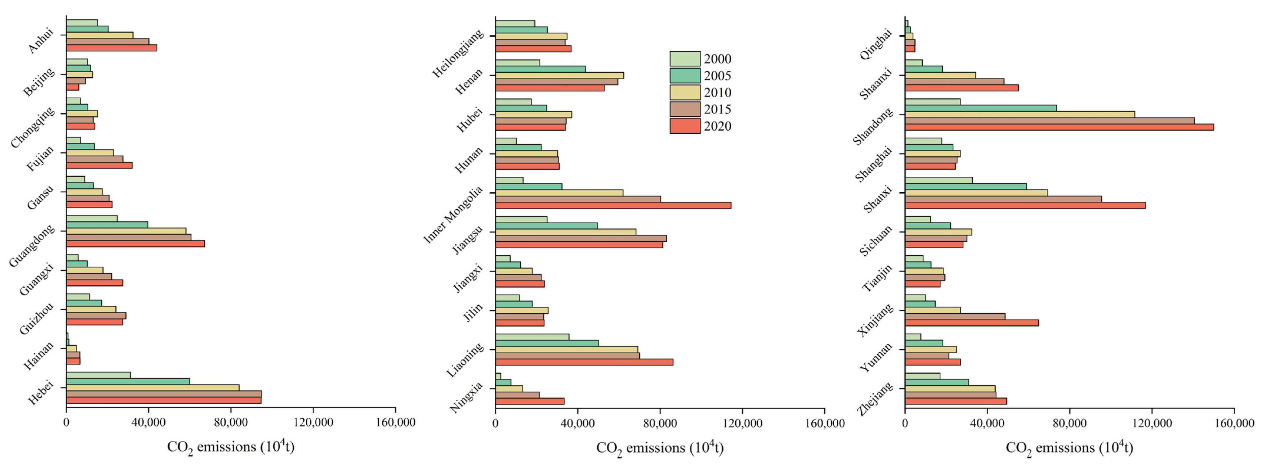
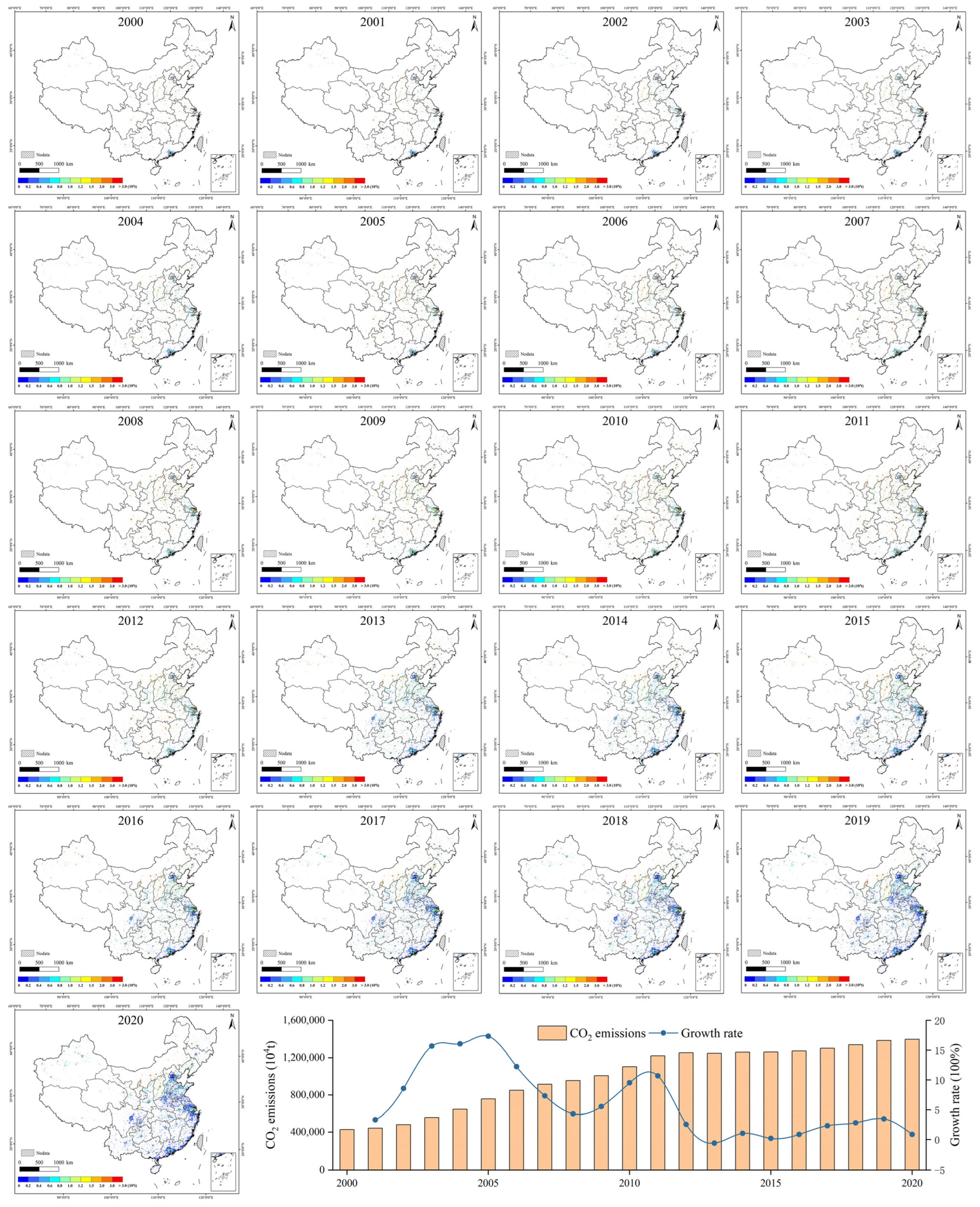
4.2.1. Variations at National and Provincial Scales

The trend in CO₂ emissions in the majority of provinces is similar to the national trend, i.e., upward (Figure 4). However, some provinces (such as Beijing, Chongqing, Henan and Shanghai) have experienced a negative growth within recent years.

There are two possible reasons for this phenomenon: first, some provinces have undergone an industrial structural transformation, which has reduced CO₂ emissions; second, some developed provinces have reduced the local CO₂ emissions by moving industries with high CO₂ emissions to other provinces [12]. At the same time, some provinces (such as Shandong, Shanxi, Hebei and Inner Mongolia) have consistently high CO₂ emissions. This is due to the developed heavy industries, high-energy consumption, and low-energy efficiency in these provinces. Among these provinces, Shandong has a well-developed heavy industry, Hebei is dominated by the steel industry, and Shanxi and Inner Mongolia produce large amounts of coal [71]. These traditional industrial provinces with strong secondary industries inevitably produce large amounts of CO₂ emissions. It is difficult to change the industrial structure of a city, so the CO₂ emissions generated by energy consumption will not decrease quickly. However, this also shows us the way: optimizing industrial structure and increasing energy efficiency is the necessary method for traditional industrial provinces to achieve emission reduction goals.

As illustrated in Figure 5, the spatial distribution of CO₂ emissions shows a significant change from 2000 to 2020. The areas of CO₂ emissions are mainly concentrated along the eastern coastal region and are relatively sparse in the western regions. The reason for this phenomenon is that the coastal areas are economically developed, with high population density and greater urbanization, resulting in intensive CO₂ emissions. As time goes on, there is an obvious expansion of CO₂ emissions and a high distribution in core urban areas and a low distribution in peripheral areas. This indicates that urbanization is increasing and that human activity is becoming more intense in core urban areas and is gradually expanding to the suburbs.

At the same time, it is shown in Figure 5 that the growth of statistical CO₂ emissions in 2020 is not significant compared to 2019. This is due to the COVID-19 pandemic in 2020 and the global economic slowdown, which has reduced the consumption of fossil fuels. However, such reductions have only slowed the growth rate of CO₂ emissions, rather than leading to a decline in statistical CO₂ emissions.

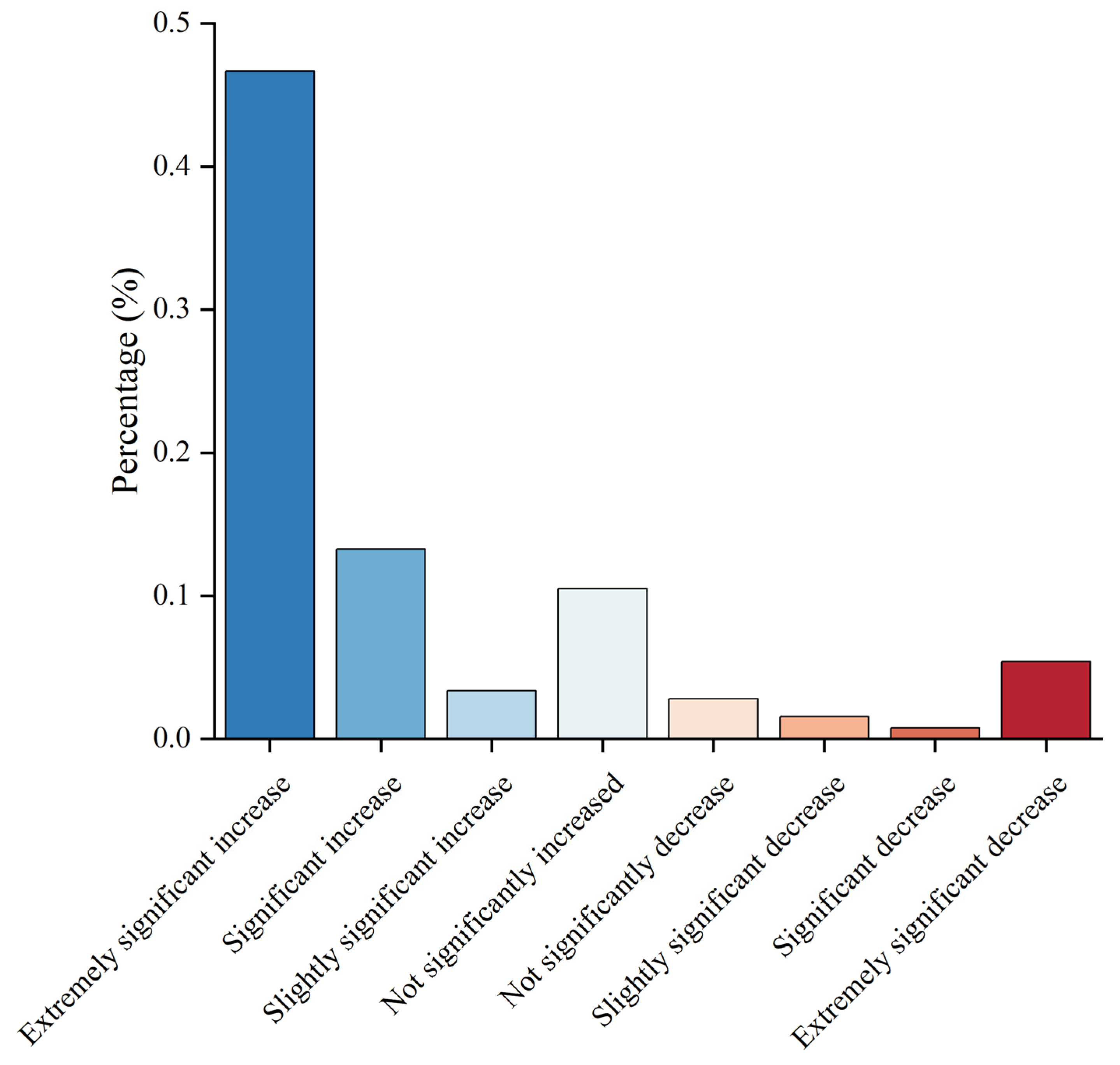
4.2.2. Study of Variation Trends at Pixel Scale

Although CO₂ emissions increased a lot in 2020 compared to 2000, in some urban core areas, CO₂ emissions showed a significant downward trend (Figure 6). Due to the increase in urbanization, the urban core cannot meet a city’s development needs and, over time, some developed cities have entered the end of their industrialization development. Many people and industries are moving to the suburbs and the urbanization of the countryside is accelerating. Based on this shift, the industrial CO₂ emissions within the core urban areas are gradually decreasing, resulting in a reduction in emissions intensity. Due to the influx of a large number of people and industries, the suburban areas inevitably consume a lot of resources, resulting in a significant increase in CO₂ emissions.

Figure 7 shows the proportion of different categories of CO₂ emissions trends. Within the total study area, the proportion of extremely significant increase is the highest (0.467%), and the proportion of significant decrease is the lowest (0.008%). The categories of significant, slightly significant and not significant increase accounted for 0.133%,0.034% and 0.105% in the study area, respectively. For the category with a decreasing trend, the highest proportion is extremely significant decrease, accounting for 0.054%. The proportion of slightly significant decrease and not significant decrease were 0.016% and 0.028%, respectively.

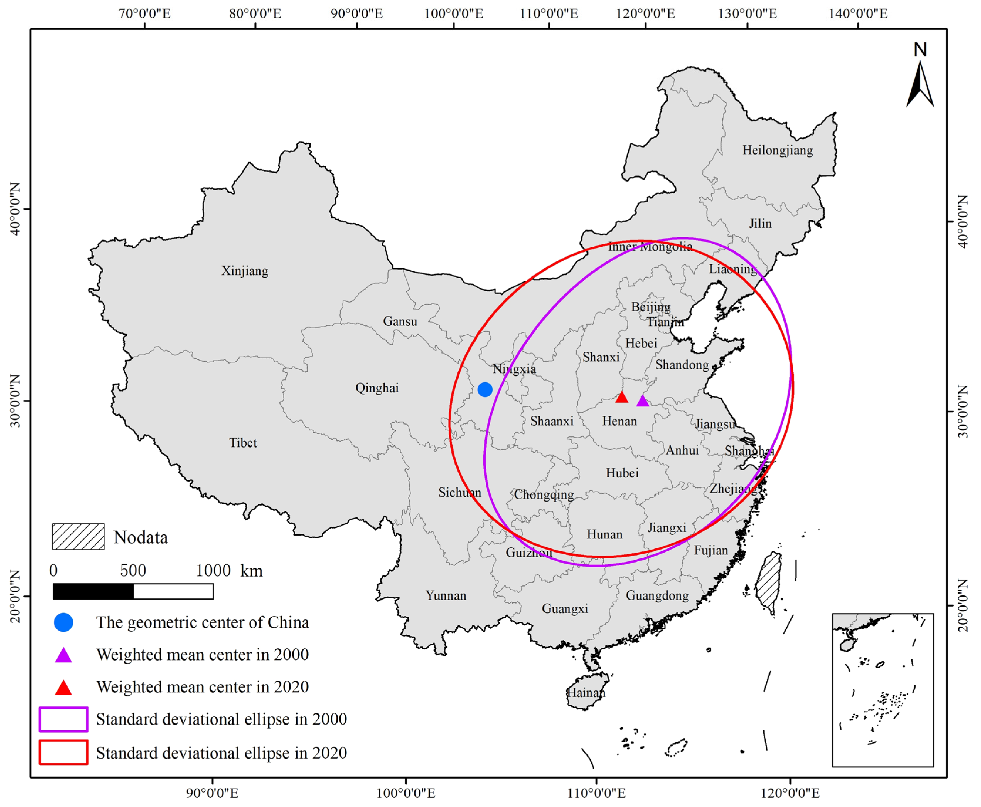
4.2.3. Evaluation of The SDE Results

In Figure 8, the SDEs almost cover the central and eastern regions in China where CO₂ emissions are concentrated. The range of CO₂ emissions in 2020 is higher than that in 2000. Furthermore, the spatial distribution of CO₂ emissions shows a pattern of northeast–southwest directional polarization, and the directional trend of CO₂ emissions in 2000 is more obvious than in 2020.

We also found that the weighted mean center of China’s CO₂ emissions is located near Henan and Shanxi, rather than in the geometric center of China’s land territory, Lanzhou. Lanzhou, located in Gansu Province, is not only the geometric center of China’s land territory, but is also a key city in the western region [72]. This indicates that CO₂ emissions are imbalanced in spatial distribution, and the CO₂ emissions are higher in the east. In terms of the movement path of the weighted mean center, the center of national CO₂ emissions is moving to the west. This change may be due to China’s “Western Development” and industrial transfer strategy. Due to its geographical location, western China is developing its economy at the expense of polluting the environment. The movement of some industries from the eastern coastal provinces to the west has enhanced local economic development, but has also generated significant CO₂ emissions. As a result, the national center of CO₂ emissions is moving to the west, and the directional trend of CO₂ emissions is weakening.

Although some scholars have simply analyzed the change of CO₂ emissions, significant analysis of trends in changes is still lacking. At the same time, few scholars have studied the migration of the weighted mean center of CO₂ emissions. The results of our innovative work have filled a gap in this field.

4.3. Driving Forces of CO₂ Emissions

To explore the drivers for CO₂ emissions, this study employed a spatial econometric model. The results for Log likelihood, Akaike info Criterion (AIC), and Schwarz Criterion (SC) are shown in

Table 4. Result of spatial economics model.

Variables	SLM			SEM
	2000	2010	2020	2000	2010	2020
Population	0.1335	0.1838	0.6918 **	0.2162	0.2395	0.6985 **
AVSI	1.2972 ***	1.1154 ***	0.9205 **	0.8983 ***	0.9851 ***	0.9275 ***
AVTI	−0.6465 *	−0.579 **	−0.9178 ***	−0.1862	−0.4202 *	−0.8458 ***
R2	0.8199	0.8141	0.6258	0.8472	0.8612	0.7072
Log likelihood	−21.4209	−18.1811	−27.5137	−19.7957	−14.758	−24.8366
AIC	52.8418	46.3623	65.0273	47.5915	37.5161	57.6733
SC	60.0117	53.5322	72.1973	53.3274	43.252	63.4093

Note: Significant at * 10% level, ** 5% level, *** 1% level.

.

AVSI significantly correlates with CO₂ emissions (Table 4), which aligns with the “high-energy consumption and high emissions” characteristics of the secondary industry. At present, the secondary sector is the main industry in China, and this will be difficult to change. This means that it will be difficult to see a significant reduction in CO₂ emissions in a short period of time because of the industrial structure. Although clean energy is being used and the industrial structure has improved in this regard, the impact of the secondary industry on CO₂ emissions is still high. Therefore, the industrial sector should continue to improve its industrial structure, in order to increase energy efficiency.

Only the population coefficient for 2020 passes the significance test at the 5% level. The results of SLM indicate that the population impact on CO₂ emissions is increasing year by year in 2000, 2010 and 2020 with coefficients of 0.13, 0.18 and 0.69, respectively. Population growth leads to more demand for food, housing, and transportation. These require more energy to meet the demands of industry, electricity, and transportation, resulting in more CO₂ emissions. These findings are also supported by other studies, which showed that the effect of population on CO₂ emissions cannot be ignored [73,74]. For some developed provinces, population size could be controlled as an effective way to control CO₂ emissions.

It is remarkable that the effect of AVTI on CO₂ emissions is always negative. This means that a strong development in the tertiary sector will help to cut CO₂ emissions. The financial and service industries are representative of the tertiary industry. These industries require less energy and produce less CO₂. This means that by keeping other variables constant, promoting the tertiary industries will help reduce CO₂ emissions. Therefore, promoting the transformation of traditional industries and supporting the development of the service and financial sectors should be the focus of government attention.

5. Conclusions

In this study, we examined the spatiotemporal dynamics of CO₂ emissions in China, and identified the regional heterogeneity of CO₂ emissions. Based on nighttime light images and MODIS NDVI data, the CO₂ emissions from 2000 to 2020 were estimated for the first time at 500 m spatial resolution in China. The model outputs showed that the proposed NUI-CV is more suitable for measuring CO₂ emissions than the traditional model (NTL). In addition, we evaluated the spatiotemporal dynamics and drivers of CO₂ emissions using the Theil–Sen and Mann–Kendall trend analysis, standard deviational ellipse and spatial econometric model.

Nationwide, China’s CO₂ emissions are distributed unevenly, with more intensive emissions in the east. This phenomenon may be related to differences in regional development. The eastern region is economically developed and consumes a large amount of fossil fuels, leading to significant CO₂ emissions. The growth rate of CO₂ emissions in 2020 shows a significant reduction due to the impact of COVID-19 pandemic. Although the total amount of CO₂ emissions continues to increase, the CO₂ emissions in urban core areas do not rise, but show a downward trend. It is inspiring evidence for the achievement of carbon reduction targets. We also found that the national center of CO₂ emissions is moving to the west, and the directional trend of CO₂ emissions is weakening. Meanwhile, AVSI and population are positively correlated with CO₂ emissions, while AVTI has a negative correlation with CO₂ emissions.

6. Policy Implications

Our research provided some inspiration for carbon emissions reduction. According to the dynamic changes of CO₂ emissions in different cities, different emission reduction measures should be formulated separately. Energy efficiency and population size should become the focus of the government. Our results confirmed that the development of the tertiary sector is the key to reducing CO₂ emissions, and thus the relevant sectors should pay attention to this. Relevant departments should formulate a series of measures to promote the transformation of traditional industries and support the development of the service and financial sectors.

In conclusion, the impact of population and secondary sector on CO₂ emissions cannot be ignored. Raising residents’ awareness of low-carbon approaches is also a crucial part of the reduction process. For underdeveloped provinces, economic growth and urbanization are the themes of development. Local governments should develop a series of policies that seek to protect the environment and develop the economy at the same time.

7. Limitations and Future Recommendations

However, there are still aspects of the study that can be improved. The first is the saturated image element problem of DMSP-OLS data, which limits their application. Although the nighttime lighting data used in this paper can solve this problem to some extent, the correction of DMSP-OLS data is the focus of upcoming research. Second, this paper only considers the population and industrial structure, and does not consider the effects of trade, policy, and capital flows on CO₂ emissions. Thus, the impact mechanisms behind CO₂ emissions still need to be further explored. We encourage scholars to study similar works of NUI-CV in other countries and regions.

References

1. Wang, S.; Zeng, J.; Huang, Y.; Shi, C.; Zhan, P. The effects of urbanization on CO2 emissions in the Pearl River Delta: A comprehensive assessment and panel data analysis. Appl. Energy 2018, 228, 1693–1706. [Google Scholar] [CrossRef]
2. Ou, J.; Liu, X.; Wang, S.; Xie, R.; Li, X. Investigating the differentiated impacts of socioeconomic factors and urban forms on CO2 emissions: Empirical evidence from Chinese cities of different developmental levels. J. Clean. Prod. 2019, 226, 601–614. [Google Scholar] [CrossRef]
3. Wang, Q.; Wang, X.; Li, R. Does urbanization redefine the environmental Kuznets curve? An empirical analysis of 134 Countries. Sustain. Cities Soc. 2021, 76, 103382. [Google Scholar] [CrossRef]
4. Wang, Q.; Wang, L.; Li, R. Trade openness helps move towards carbon neutrality—Insight from 114 countries. Sustain. Dev. 2023. [Google Scholar] [CrossRef]
5. Li, R.; Wang, X.; Wang, Q. Does renewable energy reduce ecological footprint at the expense of economic growth? An empirical analysis of 120 countries. J. Clean. Prod. 2022, 346, 131207. [Google Scholar] [CrossRef]
6. Liu, L.-C.; Cheng, L.; Zhao, L.-T.; Cao, Y.; Wang, C. Investigating the significant variation of coal consumption in China in 2002–2017. Energy 2020, 207, 118307. [Google Scholar] [CrossRef]
7. Lv, Q.; Liu, H.; Wang, J.; Liu, H.; Shang, Y. Multiscale analysis on spatiotemporal dynamics of energy consumption CO2 emissions in China: Utilizing the integrated of DMSP-OLS and NPP-VIIRS nighttime light datasets. Sci. Total. Environ. 2020, 703, 134394. [Google Scholar] [CrossRef] [PubMed]
8. Wang, Q.; Sun, J.; Pata, U.K.; Li, R.; Kartal, M.T. Digital economy and carbon dioxide emissions: Examining the role of threshold variables. Geosci. Front. 2023, 101644. [Google Scholar] [CrossRef]
9. Su, Y.; Chen, X.; Li, Y.; Liao, J.; Ye, Y.; Zhang, H.; Huang, N.; Kuang, Y. China’s 19-year city-level carbon emissions of energy consumptions, driving forces and regionalized mitigation guidelines. Renew. Sustain. Energy Rev. 2014, 35, 231–243. [Google Scholar] [CrossRef]
10. Shi, K.; Chen, Y.; Yu, B.; Xu, T.; Chen, Z.; Liu, R.; Li, L.; Wu, J. Modeling spatiotemporal CO2 (carbon dioxide) emission dynamics in China from DMSP-OLS nighttime stable light data using panel data analysis. Appl. Energy 2016, 168, 523–533. [Google Scholar] [CrossRef]
11. Koondhar, M.A.; Tan, Z.; Alam, G.M.; Khan, Z.A.; Wang, L.; Kong, R. Bioenergy consumption, carbon emissions, and agricultural bioeconomic growth: A systematic approach to carbon neutrality in China. J. Environ. Manag. 2021, 296, 113242. [Google Scholar] [CrossRef]
12. Shi, K.; Yu, B.; Zhou, Y.; Chen, Y.; Yang, C.; Chen, Z.; Wu, J. Spatiotemporal variations of CO2 emissions and their impact factors in China: A comparative analysis between the provincial and prefectural levels. Appl. Energy 2019, 233, 170–181. [Google Scholar] [CrossRef]
13. Chen, H.; Qi, S.; Tan, X. Decomposition and prediction of China’s carbon emission intensity towards carbon neutrality: From perspectives of national, regional and sectoral level. Sci. Total Environ. 2022, 825, 153839. [Google Scholar] [CrossRef]
14. Wang, S.; Fang, C.; Guan, X.; Pang, B.; Ma, H. Urbanisation, energy consumption, and carbon dioxide emissions in China: A panel data analysis of China’s provinces. Appl. Energy 2014, 136, 738–749. [Google Scholar] [CrossRef]
15. Chen, J.; Gao, M.; Cheng, S.; Hou, W.; Song, M.; Liu, X.; Liu, Y.; Shan, Y. County-level CO2 emissions and sequestration in China during 1997–2017. Sci. Data 2020, 7, 1–12. [Google Scholar] [CrossRef] [PubMed]
16. Meng, L.; Graus, W.; Worrell, E.; Huang, B. Estimating CO2 (carbon dioxide) emissions at urban scales by DMSP/OLS (Defense Meteorological Satellite Program’s Operational Linescan System) nighttime light imagery: Methodological challenges and a case study for China. Energy 2014, 71, 468–478. [Google Scholar] [CrossRef]
17. Elvidge, C.D.; Baugh, K.E.; Kihn, E.A.; Kroehl, H.W.; Davis, E.R.; Davis, C.W. Relation between satellite observed visible-near infrared emissions, population, economic activity and electric power consumption. Int. J. Remote Sens. 2010, 18, 1373–1379. [Google Scholar] [CrossRef]
18. Han, J.; Meng, X.; Zhou, X.; Yi, B.; Liu, M.; Xiang, W.-N. A long-term analysis of urbanization process, landscape change, and carbon sources and sinks: A case study in China’s Yangtze River Delta region. J. Clean. Prod. 2017, 141, 1040–1050. [Google Scholar] [CrossRef]
19. Shi, K.; Yang, Q.; Li, Y.; Sun, X. Mapping and evaluating cultivated land fallow in Southwest China using multisource data. Sci. Total. Environ. 2019, 654, 987–999. [Google Scholar] [CrossRef]
20. Su, Y.; Chen, X.; Wang, C.; Zhang, H.; Liao, J.; Ye, Y.; Wang, C. A new method for extracting built-up urban areas using DMSP-OLS nighttime stable lights: A case study in the Pearl River Delta, southern China. GIScience Remote Sens. 2015, 52, 218–238. [Google Scholar] [CrossRef]
21. Elvidge, C.D.; Sutton, P.C.; Ghosh, T.; Tuttle, B.T.; Baugh, K.E.; Bhaduri, B.; Bright, E. A global poverty map derived from satellite data. Comput. Geosci. 2009, 35, 1652–1660. [Google Scholar] [CrossRef]
22. Jean, N.; Burke, M.; Xie, M.; Davis, W.M.; Lobell, D.B.; Ermon, S. Combining satellite imagery and machine learning to predict poverty. Science 2016, 353, 790–794. [Google Scholar] [CrossRef] [PubMed]
23. Guo, W.; Lu, D.; Wu, Y.; Zhang, J. Mapping Impervious Surface Distribution with Integration of SNNP VIIRS-DNB and MODIS NDVI Data. Remote Sens. 2015, 7, 12459–12477. [Google Scholar] [CrossRef]
24. Guo, W.; Li, G.; Ni, W.; Zhang, Y.; Lu, D. Exploring improvement of impervious surface estimation at national scale through integration of nighttime light and Proba-V data. GIScience Remote Sens. 2018, 55, 699–717. [Google Scholar] [CrossRef]
25. Gong, P.; Li, X.; Wang, J.; Bai, Y.; Chen, B.; Hu, T.; Liu, X.; Xu, B.; Yang, J.; Zhang, W.; et al. Annual maps of global artificial impervious area (GAIA) between 1985 and 2018. Remote Sens. Environ. 2019, 236, 111510. [Google Scholar] [CrossRef]
26. Han, P.; Huang, J.; Li, R.; Wang, L.; Hu, Y.; Wang, J.; Huang, W. Monitoring Trends in Light Pollution in China Based on Nighttime Satellite Imagery. Remote Sens. 2014, 6, 5541–5558. [Google Scholar] [CrossRef]
27. Wang, J.; Aegerter, C.; Xu, X.; Szykman, J.J. Potential application of VIIRS Day/Night Band for monitoring nighttime surface PM 2.5 air quality from space. Atmos. Environ. 2016, 124, 55–63. [Google Scholar] [CrossRef]
28. Ji, G.; Tian, L.; Zhao, J.; Yue, Y.; Wang, Z. Detecting spatiotemporal dynamics of PM2.5 emission data in China using DMSP-OLS nighttime stable light data. J. Clean. Prod. 2019, 209, 363–370. [Google Scholar] [CrossRef]
29. Li, X.; Zhou, W. Dasymetric mapping of urban population in China based on radiance corrected DMSP-OLS nighttime light and land cover data. Sci. Total Environ. 2018, 643, 1248–1256. [Google Scholar] [CrossRef] [PubMed]
30. You, H.; Yang, J.; Xue, B.; Xiao, X.; Xia, J.; Jin, C.; Li, X. Spatial evolution of population change in Northeast China during 1992–2018. Sci. Total. Environ. 2021, 776, 146023. [Google Scholar] [CrossRef]
31. Hu, T.; Huang, X. A novel locally adaptive method for modeling the spatiotemporal dynamics of global electric power consumption based on DMSP-OLS nighttime stable light data. Appl. Energy 2019, 240, 778–792. [Google Scholar] [CrossRef]
32. Shi, K.; Chen, Y.; Yu, B.; Xu, T.; Yang, C.; Li, L.; Huang, C.; Chen, Z.; Liu, R.; Wu, J. Detecting spatiotemporal dynamics of global electric power consumption using DMSP-OLS nighttime stable light data. Appl. Energy 2016, 184, 450–463. [Google Scholar] [CrossRef]
33. Zhang, X.; Gibson, J. Using Multi-Source Nighttime Lights Data to Proxy for County-Level Economic Activity in China from 2012 to 2019. Remote Sens. 2022, 14, 1282. [Google Scholar] [CrossRef]
34. Wang, X.; Sutton, P.C.; Qi, B. Global Mapping of GDP at 1 km2 Using VIIRS Nighttime Satellite Imagery. ISPRS Int. J. Geo-Inf. 2019, 8, 580. [Google Scholar] [CrossRef]
35. Liang, H.; Guo, Z.; Wu, J.; Chen, Z. GDP spatialization in Ningbo City based on NPP/VIIRS night-time light and auxiliary data using random forest regression. Adv. Space Res. 2020, 65, 481–493. [Google Scholar] [CrossRef]
36. Shi, K.; Shen, J.; Wu, Y.; Liu, S.; Li, L. Carbon dioxide (CO2) emissions from the service industry, traffic, and secondary industry as revealed by the remotely sensed nighttime light data. Int. J. Digit. Earth 2021, 14, 1514–1527. [Google Scholar] [CrossRef]
37. Oda, T.; Maksyutov, S. A very high-resolution (1 km × 1 km) global fossil fuel CO2 emission inventory derived using a point source database and satellite observations of nighttime lights. Atmos. Chem. Phys. 2011, 11, 543–556. [Google Scholar] [CrossRef]
38. Doll, C.; Muller, J.P.; Elvidge, C. Night-time Imagery as a Tool for Global Mapping of Socioeconomic Parameters and Greenhouse Gas Emissions. Ambio 2000, 29, 157–162. [Google Scholar] [CrossRef]
39. Ghosh, T.; Elvidge, C.D.; Sutton, P.C.; Baugh, K.E.; Ziskin, D.; Tuttle, B.T. Creating a Global Grid of Distributed Fossil Fuel CO2 Emissions from Nighttime Satellite Imagery. Energies 2010, 3, 1895–1913. [Google Scholar] [CrossRef]
40. Wei, W.; Zhang, X.; Zhou, L.; Xie, B.; Zhou, J.; Li, C. How does spatiotemporal variations and impact factors in CO2 emissions differ across cities in China? Investigation on grid scale and geographic detection method. J. Clean. Prod. 2021, 321, 128933. [Google Scholar] [CrossRef]
41. Liu, X.; Ou, J.; Wang, S.; Li, X.; Yan, Y.; Jiao, L.; Liu, Y. Estimating spatiotemporal variations of city-level energy-related CO2 emissions: An improved disaggregating model based on vegetation adjusted nighttime light data. J. Clean. Prod. 2018, 177, 101–114. [Google Scholar] [CrossRef]
42. Elvidge, C.D.; Baugh, K.E.; Dietz, J.B.; Bland, T.; Sutton, P.C.; Kroehl, H.W. Radiance Calibration of DMSP-OLS Low-Light Imaging Data of Human Settlements. Remote Sens. Environ. 1999, 68, 77–88. [Google Scholar] [CrossRef]
43. Letu, H.; Hara, M.; Yagi, H.; Naoki, K.; Tana, G.; Nishio, F.; Shuhei, O. Estimating energy consumption from night-time DMPS/OLS imagery after correcting for saturation effects. Int. J. Remote Sens. 2010, 31, 4443–4458. [Google Scholar] [CrossRef]
44. Zhao, N.; Samson, E.L.; Currit, N.A. Nighttime-Lights-Derived Fossil Fuel Carbon Dioxide Emission Maps and Their Limitations. Photogramm. Eng. Remote Sens. 2015, 81, 935–943. [Google Scholar] [CrossRef]
45. Li, X.; Zhou, Y.; Zhao, M.; Zhao, X. A harmonized global nighttime light dataset 1992–2018. Sci. Data 2020, 7, 1–9. [Google Scholar] [CrossRef]
46. Letu, H.; Hara, M.; Tana, G.; Nishio, F. A Saturated Light Correction Method for DMSP/OLS Nighttime Satellite Imagery. IEEE Trans. Geosci. Remote Sens. 2012, 50, 389–396. [Google Scholar] [CrossRef]
47. Zhao, J.; Ji, G.; Yue, Y.; Lai, Z.; Chen, Y.; Yang, D.; Yang, X.; Wang, Z. Spatio-temporal dynamics of urban residential CO2 emissions and their driving forces in China using the integrated two nighttime light datasets. Appl. Energy 2019, 235, 612–624. [Google Scholar] [CrossRef]
48. Elvidge, C.D.; Baugh, K.E.; Zhizhin, M.; Hsu, F.-C. Why VIIRS data are superior to DMSP for mapping nighttime lights. Proc. Asia-Pac. Adv. Netw. 2013, 35, 62. [Google Scholar]
49. Shi, K.; Yu, B.; Hu, Y.; Huang, C.; Chen, Y.; Huang, Y.; Chen, Z.; Wu, J. Modeling and mapping total freight traffic in China using NPP-VIIRS nighttime light composite data. GIScience Remote Sens. 2015, 52, 274–289. [Google Scholar] [CrossRef]
50. Elvidge, C.D.; Zhizhin, M.; Ghosh, T.; Hsu, F.-C.; Taneja, J. Annual Time Series of Global VIIRS Nighttime Lights Derived from Monthly Averages: 2012 to 2019. Remote Sens. 2021, 13, 922. [Google Scholar] [CrossRef]
51. Shi, K.; Yu, B.; Huang, Y.; Hu, Y.; Yin, B.; Chen, Z.; Chen, L.; Wu, J. Evaluating the ability of npp-viirs nighttime light data to estimate the gross domestic product and the electric power consumption of China at multiple scales: A comparison with DMSP-OLS Data. Remote Sens. 2014, 6, 1705–1724. [Google Scholar] [CrossRef]
52. Lu, D.; Li, G.; Kuang, W.; Moran, E. Methods to extract impervious surface areas from satellite images. Int. J. Digit. Earth 2014, 7, 93–112. [Google Scholar] [CrossRef]
53. Guo, W.; Li, Y.; Li, P.; Zhao, X.; Zhang, J. Using a combination of nighttime light and MODIS data to estimate spatiotemporal patterns of CO2 emissions at multiple scales. Sci. Total. Environ. 2022, 848, 157630. [Google Scholar] [CrossRef] [PubMed]
54. Guo, W.; Lu, D.; Kuang, W. Improving Fractional Impervious Surface Mapping Performance through Combination of DMSP-OLS and MODIS NDVI Data. Remote Sens. 2017, 9, 375. [Google Scholar] [CrossRef]
55. Meng, X.; Han, J.; Huang, C. An Improved Vegetation Adjusted Nighttime Light Urban Index and Its Application in Quantifying Spatiotemporal Dynamics of Carbon Emissions in China. Remote Sens. 2017, 9, 829. [Google Scholar] [CrossRef]
56. Fang, C.; Wang, S.; Li, G. Changing urban forms and carbon dioxide emissions in China: A case study of 30 provincial capital cities. Appl. Energy 2015, 158, 519–531. [Google Scholar] [CrossRef]
57. Wang, Q.; Sun, J.; Li, R.; Pata, U.K. Linking trade openness to load capacity factor: The threshold effects of natural resource rent and corruption control. Gondwana Res. 2023, in press. [Google Scholar] [CrossRef]
58. Wang, Q.; Zhang, F.; Li, R. Free trade and carbon emissions revisited: The asymmetric impacts of trade diversification and trade openness. Sustain. Dev. 2023, in press. [Google Scholar] [CrossRef]
59. Wang, Q.; Zhang, F. The effects of trade openness on decoupling carbon emissions from economic growth–Evidence from 182 countries. J. Clean. Prod. 2021, 279, 123838. [Google Scholar] [CrossRef]
60. Chen, Z.; Yu, B.; Yang, C.; Zhou, Y.; Yao, S.; Qian, X.; Wang, C.; Wu, B.; Wu, J. An extended time series (2000–2018) of global NPP-VIIRS-like nighttime light data from a cross-sensor calibration. Earth Syst. Sci. Data 2021, 13, 889–906. [Google Scholar] [CrossRef]
61. Zhuo, L.; Zheng, J.; Zhang, X.; Li, J.; Liu, L. An improved method of night-time light saturation reduction based on EVI. Int. J. Remote. Sens. 2015, 36, 4114–4130. [Google Scholar] [CrossRef]
62. IPCC. Climate Change 2007 the Fourth Assessment Report of IPCC; Cambridge University Press: Cambridge, UK, 2007. [Google Scholar]
63. He, B.; Wu, X.; Liu, K.; Yao, Y.; Chen, W.; Zhao, W. Trends in Forest Greening and Its Spatial Correlation with Bioclimatic and Environmental Factors in the Greater Mekong Subregion from 2001 to 2020. Remote Sens. 2022, 14, 5982. [Google Scholar] [CrossRef]
64. Hu, J.; Ye, B.; Bai, Z.; Feng, Y. Remote Sensing Monitoring of Vegetation Reclamation in the Antaibao Open-Pit Mine. Remote Sens. 2022, 14, 5634. [Google Scholar] [CrossRef]
65. Villagra, P.; Rojas, C.; Ohno, R.; Xue, M.; Gómez, K. A GIS-base exploration of the relationships between open space systems and urban form for the adaptive capacity of cities after an earthquake: The cases of two Chilean cities. Appl. Geogr. 2014, 48, 64–78. [Google Scholar] [CrossRef]
66. Shi, K.; Yu, B.; Huang, C.; Wu, J.; Sun, X. Exploring spatiotemporal patterns of electric power consumption in countries along the Belt and Road. Energy 2018, 150, 847–859. [Google Scholar] [CrossRef]
67. Zhang, Q.; Yang, J.; Sun, Z.; Wu, F. Analyzing the impact factors of energy-related CO2 emissions in China: What can spatial panel regressions tell us? J. Clean. Prod. 2017, 161, 1085–1093. [Google Scholar] [CrossRef]
68. Tobler, W.R. A Computer Movie Simulating Urban Growth in the Detroit Region. Econ. Geogr. 1970, 46, 234–240. [Google Scholar] [CrossRef]
69. Kang, Y.-Q.; Zhao, T.; Yang, Y.-Y. Environmental Kuznets curve for CO2 emissions in China: A spatial panel data approach. Ecol. Indic. 2016, 63, 231–239. [Google Scholar] [CrossRef]
70. Liu, Q.; Wang, S.; Zhang, W.; Zhan, D.; Li, J. Does foreign direct investment affect environmental pollution in China’s cities? A spatial econometric perspective. Sci. Total Environ. 2018, 613, 521–529. [Google Scholar] [CrossRef]
71. Jiang, J.; Ye, B.; Liu, J. Peak of CO2 emissions in various sectors and provinces of China: Recent progress and avenues for further research. Renew. Sustain. Energy Rev. 2019, 112, 813–833. [Google Scholar] [CrossRef]
72. Xie, Y.; Ma, A.; Wang, H. Lanzhou urban growth prediction based on Cellular Automata. In Proceedings of the 2010 18th International Conference on Geoinformatics, Beijing, China, 18–20 June 2010; pp. 1–5. [Google Scholar]
73. Pappas, D.; Chalvatzis, K.J.; Guan, D.; Ioannidis, A. Energy and carbon intensity: A study on the cross-country industrial shift from China to India and SE Asia. Appl. Energy 2018, 225, 183–194. [Google Scholar] [CrossRef]
74. Shi, K.; Chen, Y.; Li, L.; Huang, C. Spatiotemporal variations of urban CO2 emissions in China: A multiscale perspective. Appl. Energy 2018, 211, 218–229. [Google Scholar] [CrossRef]
Figure 1. Study area.
Sustainability 15 13143 g001
Figure 2. Methodological framework.
Sustainability 15 13143 g002
Figure 3. Comparison of three dataset in Chengdu City; (a) NTL; (b) NUI-CV; (c) Landsat 8 OLI image with 30 m spatial resolution.
Sustainability 15 13143 g003
Figure 4. Statistical CO2 emissions by province in China.
Sustainability 15 13143 g004
Figure 5. The estimated CO2 emissions from 2000 to 2020 in China.
Sustainability 15 13143 g005
Figure 6. The spatiotemporal variations trend of CO2 emissions from 2000 to 2020.
Sustainability 15 13143 g006
Figure 7. Percentage of different categories of CO2 emissions trends.
Sustainability 15 13143 g007
Figure 8. The SDEs at provincial scale in China between 2000 and 2020.
Sustainability 15 13143 g008