Article

Integrated Reactive Power Optimisation for Power Grids Containing Large-Scale Wind Power Based on Improved HHO Algorithm

1
Hubei Engineering and Technology Research Center for AC/DC Intelligent Distribution Network, School of Electrical Engineering and Automation, Wuhan University, Wuhan 430072, China
2
Dali Power Supply Bureau of Yunnan Electric Power Grid Co., Ltd., Dali 671000, China
3
Electric Power Research Institute of Yunnan Electric Power Grid Co., Ltd., Kunming 650217, China
*
Author to whom correspondence should be addressed.
Sustainability 2023, 15(17), 12962; https://doi.org/10.3390/su151712962
Submission received: 12 July 2023 / Revised: 5 August 2023 / Accepted: 9 August 2023 / Published: 28 August 2023

Abstract

:
Large-scale wind power grid integration will greatly change the system current distribution, making it difficult for the reactive power regulator to adjust to the optimal state. In this paper, an integrated reactive power optimisation method based on the improved Harris Hawk (HHO) algorithm is proposed. Firstly, a reactive power regulation model is constructed to solve the reactive power regulation interval of wind turbines, and the reactive power margin of wind turbines is used to participate in the system’s reactive power optimisation. Finally, a reactive power compensation capacity allocation optimisation model considering nodal voltage deviation, line loss and equipment investment cost, is established, and a reactive power optimisation scheme is obtained using the Harris Hawk optimisation algorithm on the basis of considering the constraints of the wind turbine reactive power output interval. The improved HHO algorithm is used to solve the reactive power optimisation scheme considering the constraints of tidal power, machine end voltage, a conventional generator and wind farm reactive power. In the simulation, the effects of the improved Harris Hawk optimisation algorithm and the particle swarm optimisation algorithm are compared, and the experimental results prove that compared to the particle swarm algorithm, the optimisation result of the improved Harris Hawk optimisation algorithm reduces the average loss of the system by 42.6% and reduces the average voltage deviation by 30.3%, which confirms that the improved Harris Hawk intelligent optimisation algorithm is effective in proving its superiority and solving the multi-objective model for reactive power optimisation.

1. Introduction

In the context of international energy transition and global fossil energy depletion, China is vigorously promoting the development of new energy sources. Though wind power is a typical clean energy source and has been vigorously promoted [1], the power fluctuations caused by the uncertainty and uncontrollability of wind power output significantly change the system network tide distribution, making it difficult for the reactive regulator to achieve optimal operation, resulting in higher additional losses and voltage overrunning in the system.
The basic research idea for reactive power optimisation problems is to select multiple control variables, construct a reactive power optimisation model, set the objective function, constraints, and, finally, select different algorithms for iterative solutions [2,3,4,5]. The algorithms used to find the reactive power optimisation model are divided into two main categories: one category the traditional reactive power optimisation algorithm [6,7,8], and the other category is the heuristic intelligent optimisation algorithm [9,10,11,12,13].
In terms of traditional optimisation algorithms used to solve reactive power optimisation problems, the literature [14] uses a linear programming method to solve the model by coordinating the control of SVGs in MV distribution networks with distributed PV inverters in LV distribution networks. The literature [15] proposed a two-stage algorithm for dynamic reactive power optimisation based on the decoupled interior point method and mixed integer programming. In the literature [16], a two-stage dynamic reactive power optimisation model is proposed for the reactive power optimisation problem of mixed integer non-linear programming. A mixed integer programming model with the number of reactive power control device actions being a constraint is constructed in the literature [17] to decide the solution. The above traditional optimisation algorithms also have certain problems when solving reactive power optimisation problems, such as sensitivity to initial conditions, high computational complexity and the need for large amounts of data. To address the shortcomings of the above traditional optimisation algorithms in solving reactive power optimisation problems in power systems, heuristic intelligent optimisation algorithms are increasingly used in reactive power optimisation problems due to their strong convergence and global and local optimisation capabilities. In [18], a reactive power optimisation model for a distribution network with wind turbines was constructed and solved using particle swarm algorithms. In [19], the authors constructed an objective function based on the operating cost of the system to validate the grey wolf algorithm, and the improved grey wolf algorithm improved the convergence of the algorithm and the ability of local optimisation. In [20], a two-layer optimisation model of distribution network with DG was constructed, with DG investment and the operation cost being the upper-level objective and distribution network line loss and voltage deviation being the lower-level objectives, and the sparrow optimisation algorithm was improved and solved. In [21], the authors construct the objective functions of maximum active power, total voltage harmonic distortion rate and minimum voltage deviation for PV grid connection, solving them using an ant colony algorithm improved through adaptive weighting.
In conclusion, most of the literature on reactive power optimisation of new energy wind power grids fails to analyse the voltage weaknesses of the grid and ignores the reactive power regulation capability of the wind farm itself. The identification of voltage weak nodes can target the installation of reactive power compensation equipment, which, in turn, reduces the dimensionality of the optimisation variables and the difficulty of solving reactive power optimisation problems. The reactive power margin of the wind turbine can replace part of the reactive power compensation device to ensure reactive power regulation and improve the overall economy of the system.
To solve the above problems, this paper proposes an integrated reactive power op-timisation method for large-scale wind power grids based on the improved HHO algo-rithm. The method, firstly, identifies the voltage weak points of wind farms after grid con-nection using the continuation power flow method and places reactive power compensation devices at the weak points to reduce the dimensions of optimisation variables. Secondly, the reactive power margins of doubly fed wind turbines are analysed and used for reactive power optimisation to improve the economy of the system. The HHO algorithm is then improved using various strategies to improve its convergence, as well as global and local optimisation capabilities, and, finally, an integrated reactive power optimisation strategy is obtained by solving the objective function, with node voltage deviation, line losses and equipment investment cost used as indicators. The superiority of the improved Harris Hawk intelligent optimisation algorithm in solving the multi-objective model for reactive power optimisation is verified by comparing the results of the Harris Hawk optimisation algorithm before and after the improvement to those of the particle swarm optimisation algorithm.

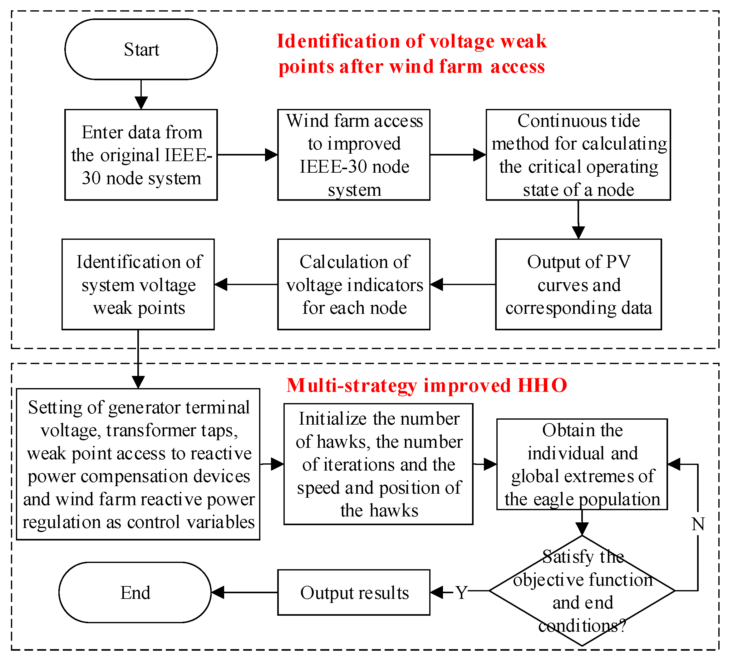
2. Integrated Reactive Power Optimisation Model Construction and Solution

The main process of establishing and solving the integrated reactive power optimisation model for a large-scale wind power grid based on the improved HHO algorithm proposed in this paper is as follows:
  • Determine the voltage weak nodes of the system based on the continuous flow method and use the identified voltage weak nodes as the access points of reactive power compensation equipment.
  • Analyse the reactive power regulation margin of the doubly fed turbine and use it as one of the optimisation variables to perform reactive power optimisation.
  • For actual wind farms, the comprehensive reactive power optimisation solution model is constructed by considering the current constraints and the inequality constraints on the constraint control variables, with the node voltage deviation, line loss and equipment investment cost being the objective functions.
  • Use the multi-strategy improved HHO algorithm to solve the comprehensive reactive power optimisation model and analyse the results.
The overall flow of the example analysis is shown in Figure 1.

3. Integrated Reactive Power Optimisation Method Considering Turbine Reactive Power Regulation Margins

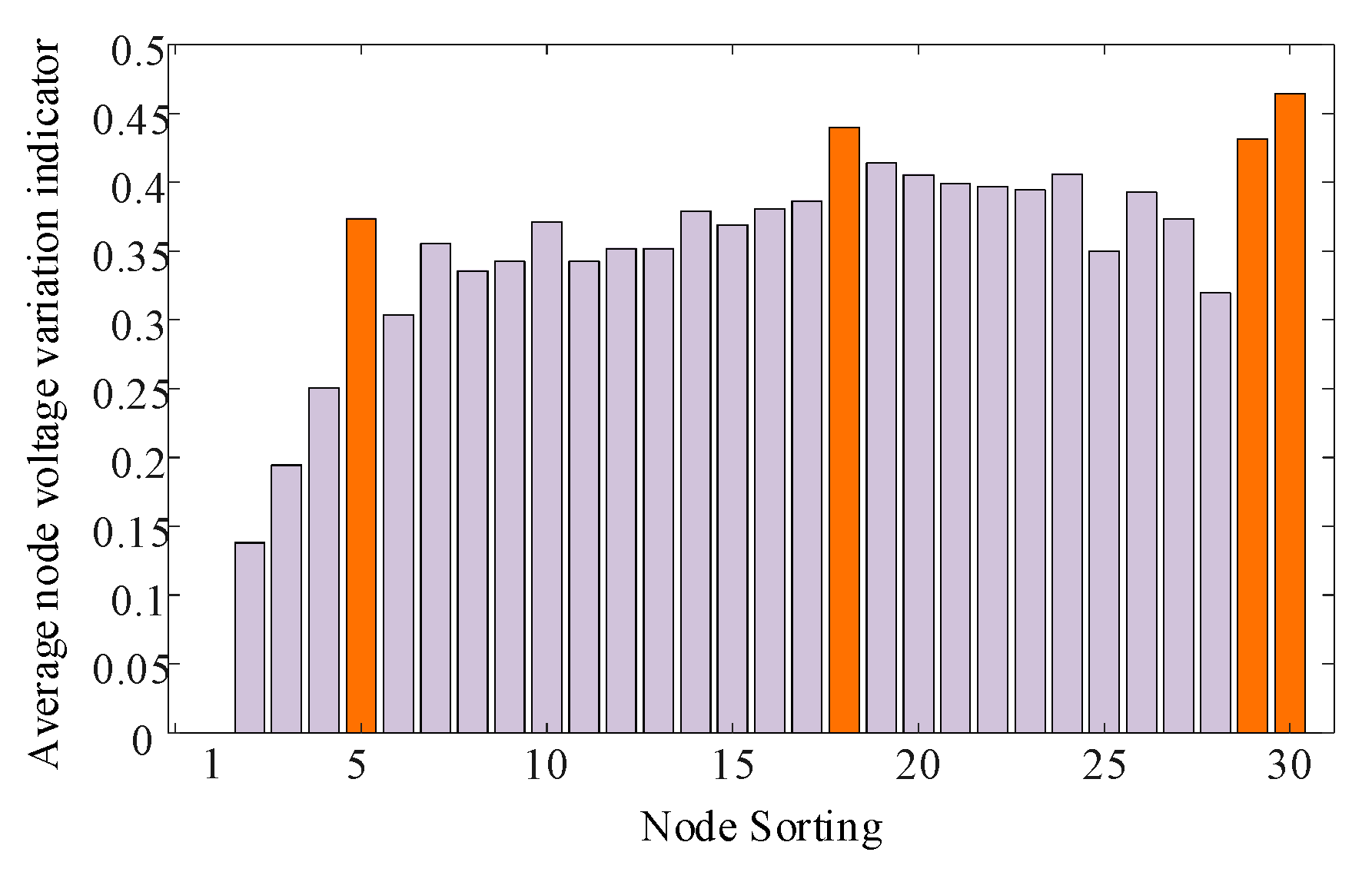
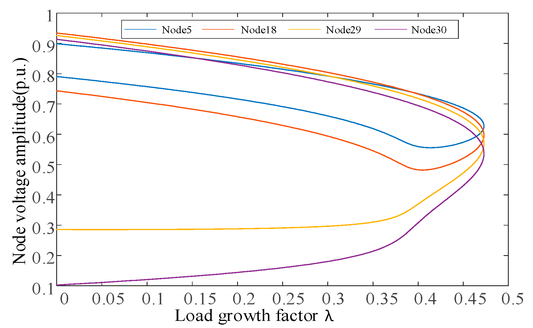
3.1. Identification of System Voltage Weak Points Based on the Continuation Power Flow Method

When large-scale new energy wind farms are connected to the grid, the power fluctuations caused by the uncertainty and uncontrollability of their power output will significantly affect the tidal wave distribution of the system, and the voltage at each node will fluctuate, while voltage instability in the grid often starts from one or a few weak nodes with stable voltages, which then spreads to other nodes [22]. By identifying voltage weak points through research, reactive power can be optimised for these weak points, thereby reducing the dimensionality of the variables in the reactive power optimisation model and improving the efficiency of the optimisation.
The basic model of the continuation power flow method is the extended tide equation, which determines whether the current state is stable by analysing the various state indicators of the system in the critical operating state, as the operating state when the transmission power of a branch reaches the maximum transmission power is the critical operating state.
Let the tidal equation for the system in n dimensions with parameters be
f ( x , λ ) = 0
where x is the node voltage amplitude and the phase angle in the system, and λ is the load growth factor.
The continuation power flow method is used to overcome the singularity of the Jacobi matrix by incorporating a load growth factor to obtain a complete PV curve for the node, where the continuation power flow method consists of four parts: parameterisation, prediction, step and correction [23,24].
The PV curve visualises the voltage variation at each node in the power transfer critical point state for the access of doubly fed wind turbines.
Let the voltage variation indicator for node i be
Δ V i = V i 0 V cri V i 0 × 100 %
where V i 0 is the initial voltage of node i after the doubly fed turbine is connected to the system, and V cri is the voltage corresponding to node i in the critical state.
The greater the node voltage variation indicator, the more vulnerable the node voltage and the greater the need for some reactive power compensation for voltage optimisation at the node.

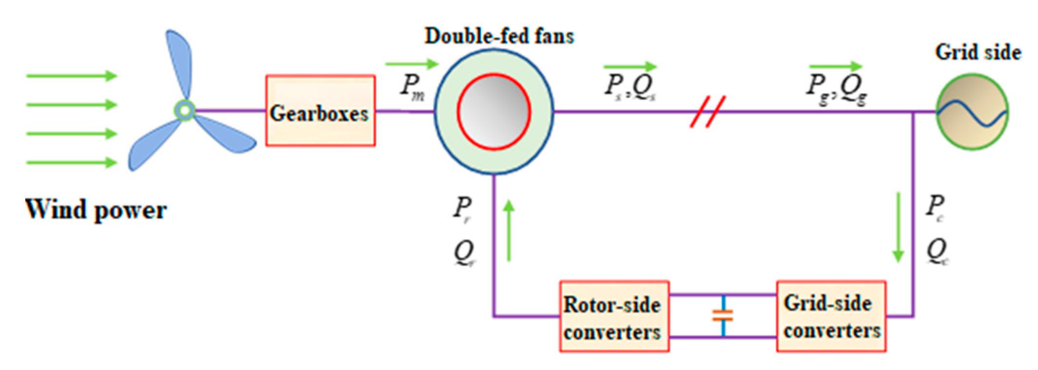
3.2. Analysis of Reactive Power Regulation Margins for Doubly Fed Wind Turbines

In this paper, doubly fed asynchronous wind turbines are used as the wind turbine type in wind farms and analysed. In normal operation, doubly fed asynchronous wind turbines have a certain adjustment range of reactive power, which can be used as a new type of reactive power source to support the reactive power optimisation of the power grid in order to improve the efficiency of the reactive power optimisation of the power system [25,26,27].
The relationship between the active power P g absorbed by the converter on the grid side, the active power P r absorbed on the rotor side and the active power P s emitted on the stator side during normal operation of a doubly fed fan is satisfied by
P g = P r = s P s
where s is the rate of rotation of the rotor side of the doubly fed fan.
The power transfer and conversion model of a doubly fed fan is shown in Figure 2. For a conventional doubly fed fan, the stator-side reactive power range is as follows:
Q s min Q s Q s max
where Q s is the reactive power emitted from the stator side of the doubly fed fan, Q s min is the maximum reactive power absorbed by the stator side of the doubly fed fan, and Q s max is the maximum reactive power emitted from the stator side of the doubly fed fan.
During normal operation, the voltage at the machine end of a doubly fed fan is approximately constant, but as the active power output to the grid side increases, the reactive power available for regulation within the doubly fed fan decreases. The reactive power output range is directly related to the reactive power regulation capability of the stator-side and grid-side converters, being formatted as follows:
Q g . max = Q s . max + Q c . max Q g . min = Q s . min + Q c . min
where Q g . max and Q g . min are the maximum and minimum values of the reactive power injected into the grid side of the doubly fed wind turbine, respectively; Q c . max and Q c . min are the maximum and minimum values of the reactive power of the converter on the grid side of the doubly fed wind turbine, respectively; and Q s . max and Q s . min are the maximum and minimum values of the reactive power output on the stator side of the doubly fed wind turbine, respectively.
Q s r . max = ( 3 L m 2 L s U s I r . max ) 2 ( P m 1 s ) 2 3 U s 2 2 ω L s Q s r . min = ( 3 L m 2 L s U s I r . max ) 2 ( P m 1 s ) 2 3 U s 2 2 ω L s
Q s s . max = ( U s I s . max ) 2 ( P m 1 s ) 2 Q s s . min = ( U s I s . max ) 2 ( P m 1 s ) 2
where L s is the stator-side inductance of the doubly fed fan; L m is the excitation inductance of the doubly fed fan; U s is the rms value of the stator voltage of the doubly fed fan; s is the turndown rate on the rotor side of the doubly fed fan; and I s . max and I r . max are the maximum current values on the stator and rotor sides of the doubly fed fan, respectively; and Pm is the input mechanical power of the doubly fed fan to the grid.
The main factor affecting the reactive power regulation range of the grid-side converter is the size of the grid-side converter capacity, as shown in the following equation:
Q c . max = S c . max 2 ( P m 1 s ) 2 Q c . min = S c . max 2 ( P m 1 s ) 2
where S c . max is the rated capacity of the converter on the grid side of the doubly fed wind turbine, Pm is the input mechanical power of the doubly fed turbine to the grid, and s is the turndown rate on the rotor side of the doubly fed turbine.
In summary, once the current wind speed and wind power of the wind farm are known, the reactive power regulation range of the entire wind farm can be calculated based on the reactive power regulation model of the doubly fed asynchronous wind turbine in the wind farm. The reactive power margin of the wind farm can then be applied to the reactive power optimisation problem of the power grid to give full play to the reactive power regulation characteristics of the wind farm and ensure the safe and stable operation of the power grid.

3.3. Formulation of Optimisation Problem

3.3.1. Objective Function

The construction is designed to minimise system voltage deviations, line losses and the total investment cost of reactive equipment (capacitor banks) at the nodes to be compensated, which can be expressed as follows:
min f 1 ( x ) = v = 0 M ( U v U N ) 2 min f 2 ( x ) = i , j N L g i j ( U i 2 + U j 2 2 U i U j cos θ i j ) min f 3 ( x ) = w = 1 3 m w C w
where M is the number of nodes in the system; v is the node number; Uv is the actual voltage value of the node at the moment; UN is the rated voltage value of the node; Ui, Uj and θ ij are the voltage magnitudes of nodes i and j, respectively, and the phase angle difference between the two nodes; NL is the set of all branches in the system; w is the reactive compensation node number, m is the cost of each capacitor bank and C is the number of capacitor banks connected to the reactive compensation node; and f 1 ( x ) is a function of voltage deviation and optimisation variables, f 2 ( x ) is a function of line losses and optimisation variables, and f 3 ( x ) is a function of the investment cost of reactive power compensation equipment and optimisation variables.

3.3.2. Flow Constraints

The Flow Constraints are that the injected power is equal to the outgoing power at each node of the power system during operation.
P i U i j = 1 n U j ( G i j cos θ i j + B i j sin θ i j ) = 0 Q i U i j = 1 n U j ( G i j sin θ i j + B i j cos θ i j ) = 0
where Pi and Qi are the active and reactive power at node i; Ui, Uj and θ ij are the voltage amplitudes at nodes i and j and the phase angle difference between the two nodes, respectively; and Gij and Bij are the conductance and conductance before nodes i and j.

3.3.3. Inequality Constraints

Power system in the operation process to ensure stable operation of the system, voltage fluctuations need to meet certain requirements, at the same time as a means of voltage regulation, transformer taps and capacitor access capacity also exists in a certain range of limitations.
U G i min U G i U G i max T i min T i T i max Q C i min Q C i Q C i max
where the inequality constraint contains the voltage UGi at node i of the generator, and UGimin and UGimax are the minimum and maximum values of the voltage at the generator, respectively; Ti, Timin and Timax are the highest and lowest tap positions of the on-load regulator transformer, respectively; and QCi, QCimin and QCimax are the maximum and minimum compensation capacities of the capacitor bank and the compensation capacity of the reactive power compensation capacitor throw, respectively.
The reactive power output QGi of the generator and the reactive power QFi of the doubly fed wind turbine are also subject to the same maximum and minimum value constraints as the following equation:
Q G i min Q G i Q G i max Q F i min Q F i Q F i max

4. Integrated Reactive Power Optimisation Model Solving Based on the Improved HHO Algorithm

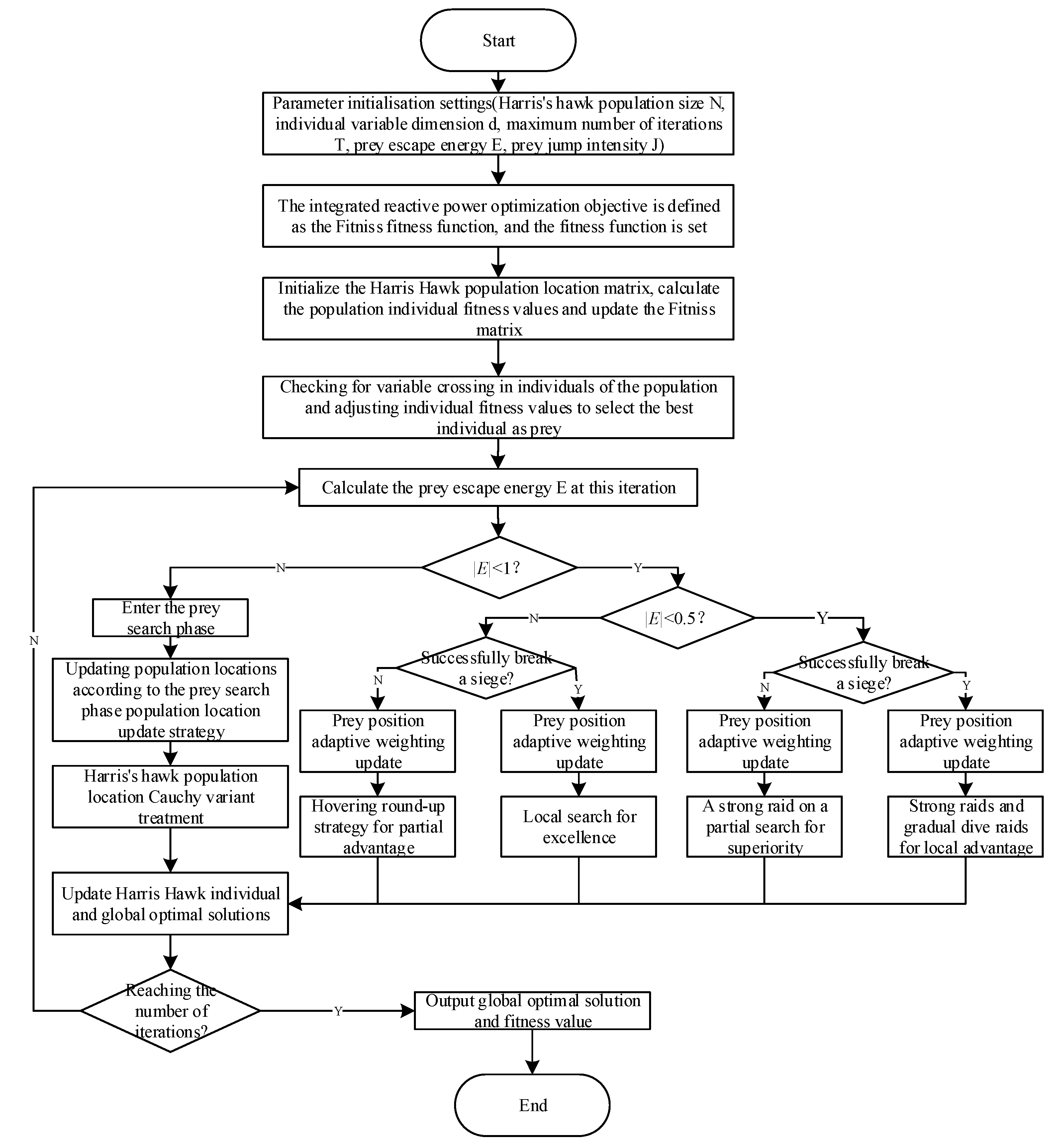
4.1. Conventional HHO Algorithm

Harris Hawks Optimisation (HHO) is a novel bionic intelligent optimisation algorithm proposed by Ali Asghar Heidari and Seyedali Mirjalili in 2019 [28]. The algorithm mimics the Harris Hawk predation characteristics and combines Levy flight functions to achieve solutions to complex multidimensional problems [29,30].

4.1.1. Harris Hawk Population Initialisation Settings

In the simulation experiment, a virtual population of Harris Hawks is required to hunt prey, and we assume a population of Harris Hawks of size N of E a g l e = ( X 1 , X 2 , , X N ) T . The initial position of its population can be represented by the following matrix:
X E a g l e = x 1 , 1 x 1 , 2 x 1 , d x 2 , 1 x 2 , 2 x 1 , d x N , 1 x N , 2 x N , d
where, N is the total number of eagles in the Harris Hawk population, d is the number of variables included in each Harris Hawk population, the dimensionality of the optimisation problem and X i , j is the value of the jth dimension for the ith Harris Hawk.
Based on the practical aspects of the above optimisation problem, the eagle can be defined as follows:
E a g l e = ( U G 1 , U G N 1 , T 1 , T N 2 , C 1 , C N 3 , Q 1 , Q N 4 ) T
where U G is the terminal voltage of a conventional generator set, N 1 is the number of conventional generator sets, T is the tap position of the load-ratio voltage transformer, N 2 is the number of load-ratio voltage transformer, C is the number of capacitors used to perform reactive power compensation, N 3 is the number of capacitor banks used to perform reactive power compensation, Q is the reactive power margin used by the wind farm used to perform reactive power regulation and N 4 is the number of wind farms.
To evaluate the fitness value of each Harris Hawk, a target matrix was used to store the fitness value of each Harris Hawk during the search for excellence, as shown in Equation (15):
F i t n e s s ( X 1 , X 2 , , X N ) = f ( [ X 1 , 1 , X 1 , 2 , , X 1 , d ] ) f ( [ X 2 , 1 , X 2 , 2 , , X 2 , d ] ) f ( [ X N , 1 , X N , 2 , , X N , d ] )
where N is the total number of eagles in the Harris eagle population, and d is the number of variables included in each Harris eagle population, i.e., the dimensionality of the optimisation problem.

4.1.2. Prey Search Phase

Harris Hawks choose different predatory behaviour depending on the escape energy of their prey, which is represented as E, as shown in Equation (16):
E = 2 E 0 ( 1 t T )
where E is the escape energy of the prey at the current number of iterations, E 0 is a random number between −1 and 1, t is the current number of iterations, and T is the set maximum number of iterations for the Harris Hawk population.
Assuming that the two random prey species are random prey 1 and random prey 2, while setting the maximum number of iterations for the Harris Hawk population at 300, the adaptive decay phenomenon of the escape energy of the two random prey species with increasing number of iterations is shown in Figure 3.
The absolute value of prey escape energy decreases with the number of iterations, as well as when the absolute value of prey escape energy is greater than 1, indicating that the prey is physically abundant and the Harris Hawk is far away from the prey; the Harris Hawk population will use individuals within the population to disperse their flight and search for prey in a larger area. A random number is used to define whether Harris Hawks find prey during the search phase and select the next iteration of the location update strategy, as shown in Equations (17) and (18):
X m ( t ) = 1 N i = 1 N X i ( t )
where X m ( t ) is the average position of the Harris Hawk population at the time of the tth iteration, N is the total number of hawks in the Harris Hawk population and X i ( t ) is the position of the ith Harris Hawk at the time of the tth iteration.
X ( t + 1 ) = X r a n d ( t ) r 1 X r a n d ( t ) 2 r 2 X ( t ) p 0.5 ( X r a b b i t ( t ) X m ( t ) ) r 3 ( L B + r 4 ( U B L B ) ) p < 0.5
where X ( t + 1 ) is the position vector of a Harris Hawk at the next iteration; X r a b b i t ( t ) is the position vector of the prey in the current iteration; X m ( t ) is the average position of the Harris Hawk population at the time of the tth iteration; X r a n d ( t ) is the position of a random individual in the Harris Hawk population at the time of the tth iteration; UB and LB are the maximum and minimum values of the dimensional variables, respectively; X ( t ) is the position vector of the Harris Hawk at the current iteration; and r 1 , r 2 , r 3 , r 4 and p are random numbers in the range 0–1.
In summary, during the prey search phase, Harris Hawks update their position for the next iteration based on the magnitude of the value. If p 0.5 , it means that none of the Harris Hawks in the population have found a prey position, so one of the other hawks in the population will be randomly selected for the position update. If p < 0.5 , it means that one Harris Hawk in the population has found prey, meaning that the next iteration position will be updated with the prey position for roundup hovering.

4.1.3. Prey Hunting Phase

When the prey is found and circled by the Harris Hawk population, the hawk population will conduct a prey siege when the absolute value of the prey’s escape energy E is less than 1. Depending on the prey’s escape energy, the colony will choose a different strategy for rounding up the prey, which will include circling roundup, strong assault, circling roundup with progressive dive assault and strong assault with progressive dive assault.
When the prey escape energy E satisfies 0.5 < E < 1 , the prey still has some energy to escape, meaning that the Harris Hawk flock roundup strategy will be a circling roundup, as shown in Equations (19) and (20):
X ( t + 1 ) = Δ X ( t ) E J X r a b b i t ( t ) X ( t )
Δ X ( t ) = X r a b b i t ( t ) X ( t )
where X ( t + 1 ) is the position vector of the Harris Hawk at the next iteration; Δ X ( t ) is the position distance between the prey and the Harris Hawk at the current iteration; J is a random number in the range 0–2 representing the random jump strength of the prey, which varies randomly at each iteration to restore the chance of the moment when the capture occurs; and E is the escape energy of the prey at the current iteration.
When the prey escape energy E satisfies E < 0.5 , the prey escape energy is about to be depleted, meaning that the Harris Hawk flock roundup strategy is a strong surprise attack, as shown in Equation (21):
X ( t + 1 ) = X r a b b i t ( t ) E Δ X ( t )
where X ( t + 1 ) is the position vector of the Harris Hawk at the next iteration, Δ X ( t ) is the position distance between the prey and the Harris Hawk at the current iteration, E is the escape energy of the prey at the current iteration, and X r a b b i t ( t ) is the position vector of the prey at the current iteration.
When the prey escape energy E satisfies 0.5 < E < 1 and successfully breaks through the flock’s siege, in order to simulate the behaviour of the prey during the escape phase, levy flight is introduced into the HHO algorithm to simulate the irregular behaviour of the prey during the escape phase, meaning that the Harris Hawk flock’s siege strategy at this time is a circling siege with a gradual swooping assault, in which the hawks will evaluate the next siege strategy based on Equation (22):
Y = X r a b b i t ( t ) E J X r a b b i t ( t ) X ( t )
The Harris Hawk will check the prey’s position against its own to see if the last hawk siege was a valid act, and if it was not a valid act, it will perform an irregular progressive swoop based on levy flight and update its position, as shown in Equation (23):
Z = Y + S L F ( d )
where Z is the Harris Hawk’s position vector for the next iteration based on the levy flight update, S is a random position increment of dimension 1 × d , and LF is the levy flight function.
In summary, the positional fitness values of Z and Y need to be compared to determine the position of the Harris Hawk population after the next iteration of the update, as shown in Equation (24):
X ( t + 1 ) = Y F i t n i s s ( Y ) < F i t n i s s ( X ( t ) ) Z F i t n i s s ( Z ) < F i t n i s s ( X ( t ) )
When the prey escape energy E satisfies E < 0.5 and the flock has successfully broken through the hawk roundup, the hawks move using a similar strategy and circling roundup and gradual swoop assault, but at this point, the prey’s escape energy is considered to be small, and a strong assault with a gradual swoop assault is adopted. The strategy needs to be updated to reduce the average distance between the hawks and the prey, as shown in Equation (25):
Y = X r a b b i t ( t ) E J X r a b b i t ( t ) X m ( t )
The position of the Harris Hawk flock after the next iteration of the update is structured as shown in Equation (24).

4.2. Improved HHO Algorithm

The main parameters that affect the ability of the conventional HHO algorithm are the prey jump strength and the prey escape energy. When the jump strength is small, the algorithm may fall into the local optimum and vice versa, but too large a jump strength directly reduces the search accuracy of the global optimum, while the change in prey escape energy directly affects the search efficiency of the algorithm. In response to the search efficiency and local optimum problems that still exist in the conventional HHO algorithm, this paper makes algorithmic improvements to it from multiple perspectives. The improved HHO algorithm has a stronger search capability and is faster than the conventional HHO and previous algorithms used in power system reactive power optimisation, and the strategy used to improve the conventional HHO algorithm in this paper is described below.

4.2.1. Corsi Variation in the Harris Hawk Population

To address the problem of easily falling into local optima in the conventional HHO algorithm, a Cauchy Distribution is used to diversify the Harris Hawk population to increase the search space of the Harris Hawk population and improve the global optimal search capability of the HHO algorithm, where the standard Cauchy distribution function is structured as shown in Equation (26):
f ( x ) = 1 π ( 1 x 2 + 1 )
When the HHO algorithm finishes updating the global optimal solution X b e s t after each iteration, the global optimal solution X b e s t is subjected to a Corsi variation, as shown in Equation (27):
X b e s t ( t + 1 ) = X b e s t ( t ) + X b e s t ( t ) C a u c h y ( 0 , 1 )
where X b e s t ( t + 1 ) is the global optimal solution when the next iteration is performed, X b e s t ( t ) is the global optimal solution generated in this iteration, and C a u c h a y ( 0 , 1 ) is the number of dimensions of the corresponding variable, i.e., d. Corsi variance factors were generated to update the range of each dimension in the original global optimal solution.

4.2.2. Prey Jump Strength Optimisation

The prey jump strength J in the conventional HHO algorithm is a random number in the range 0–2, but in reality, the prey jump strength should be related to the prey’s real-time escape energy E. Therefore, the prey jump strength in the conventional HHO algorithm needs to be optimised by replacing the upper limit of the prey jump strength in each iteration with a dynamic upper limit that combines the real-time escape energy, thus restoring the actual situation when the prey escapes and helping to enhance the global optimisation capability of the algorithm.
The prey jump intensity is optimised as shown in Equation (28):
J = J 0 ( 1 + 2 E 0 ( 1 t T ) )
where J is the initial prey jump strength value in the range 0–1, E is a random number between −1 and 1, t is the current number of iterations, T is the set maximum number of iterations for the Harris Hawk population, and J is the jump strength that has been optimised in real time using the prey escape energy.
After the prey jump strength has been realised in real time by combining the escape energy, the jump strength changes in real time with the increase in the number of iterations, following the change in the prey’s own escape energy, as shown in Figure 4. In the early iterations of the HHO algorithm, the jump range is large, but as the number of iterations increases, the prey’s escape energy adaptively decays, meaning that the jump intensity decreases in the later iterations. Therefore, the optimisation of the jump strength helps to enhance the global search capability of the algorithm in the early iterations and the local search capability in the late iterations.

4.2.3. Prey Position Adaptive Weighting Update

The conventional HHO algorithm is divided into four predation strategies based on the different ranges of values of the prey’s escape energy E. The use of adaptive weight coefficients to update the position of the prey X r a b b i t ( t ) is proposed during the iteration of the algorithm, and the processing can improve the algorithm’s local search capability. The adaptive weight coefficients and prey position updates are given in Equations (29) and (30):
ω t = sin ( π t 2 T + π ) + 1
X r a b b i t ( t + 1 ) = ω t X r a b b i t ( t )
where ω t is the adaptive weighting factor for the prey position updated in this iteration, X r a b b i t ( t + 1 ) is the prey position in the next iteration updated based on the adaptive weighting factor, and X r a b b i t ( t ) is the prey position in this iteration not processed based on the adaptive weighting factor.

4.3. Integrated Reactive Power Strategy Solving Process Based on Improved HHO Algorithm

In this paper, the generator end voltage, on-load adjustable transformer taps, reactive power compensation equipment at voltage weak points and wind farm reactive power regulation margin are taken as variables that need to be optimised, i.e., X in the improved HHO optimisation algorithm, as well as the objective function, which takes into account the node voltage deviation, line loss and equipment investment cost, is taken as the value of the optimisation algorithm’s fitness function in order to enact the solution of the algorithm. In summary, the solution flow of the improved integrated reactive power optimisation strategy based on the HHO algorithm proposed in this section is shown in Figure 5.
(1)
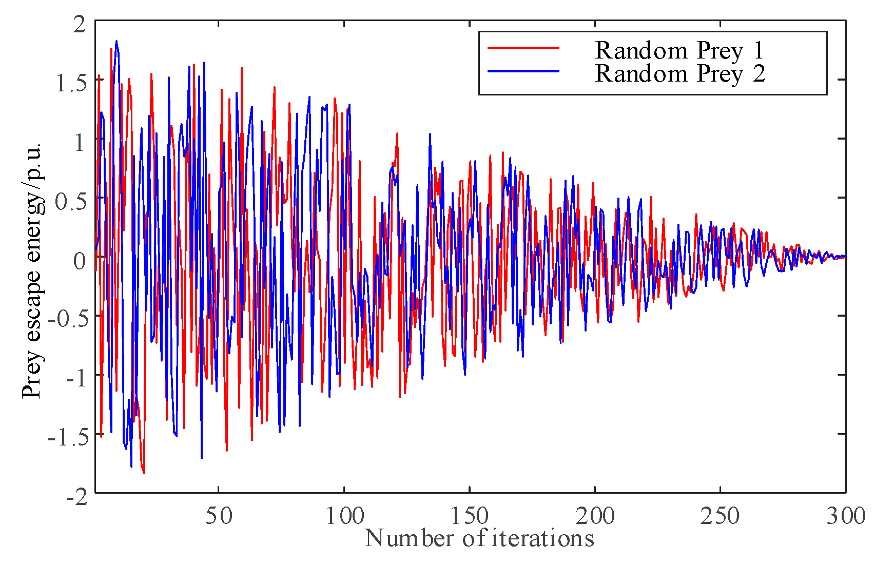
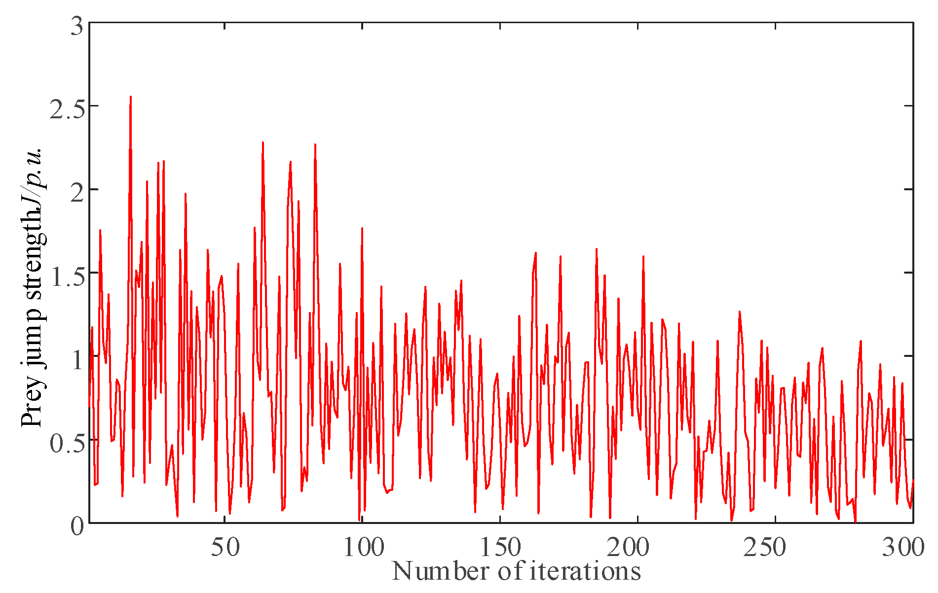
Population initialisation and parameter setting: The population size of Harris Hawk is set as N, the dimension of the variables contained in Harris Hawk individuals is set as d, and the maximum number of iterations is set as T. We then initialize the prey escape energy E and jump strength J , initialize the location of Harris Hawk population individuals, define the integrated reactive optimisation objective as the fitness function and calculate the fitness value of the initialised solution.
(2)
The locations of individuals in the population are tested for dimensional variable crossing limits, individual fitness values are calculated and adjusted, the optimal individual is selected as prey, and the prey escape energy at the current number of iterations is updated based on Equation (16).
(3)
The next location update strategy for the Harris Hawk population is decided based on the prey escape energy size, and if the absolute value of prey escape energy is greater than 1, the prey search phase is carried out, and the Harris Hawk population’s location Corsi variation is processed based on Equation (27).
(4)
If the absolute value of prey escape energy is less than 1, the prey roundup phase is carried out, and different location update strategies are then selected according to whether the absolute value of prey escape energy is greater than 0.5 and whether the prey breaks through the last roundup of the Harris Hawk population, allowing us to carry out local optimisation of the algorithm.
(5)
Adaptive weighting of the prey position is determined based on Equation (30), the jump strength of the prey for this iteration is determined based on Equation (28), and the position of the next iteration of the Harris Hawk population is updated based on the processed prey position. The fitness value of the new population individuals is calculated, and the global optimal solution is updated.
(6)
We determine whether the number of iterations satisfies the maximum number of iterations, and if so, we output the global optimal solution and the best fitness value for the Harris Hawk population; if not, the maximum number of iterations is transferred to step (2).

5. Results and Discussion

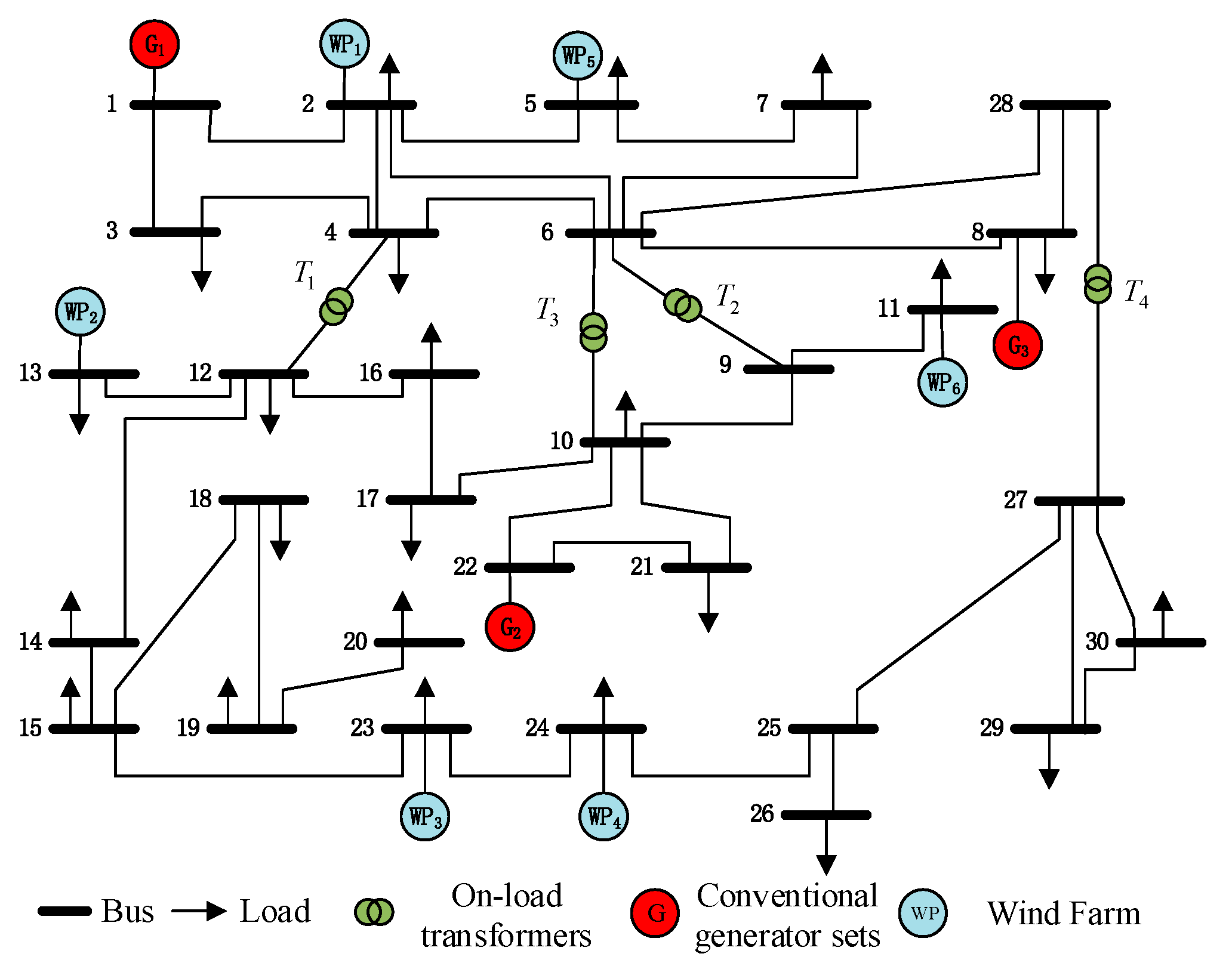
5.1. System Description

The computer used was an 11th Gen Intel(R) Core(TM) i5-11400H @2.70 GHz model with Windows 10 Home Edition, and the simulation modelling software used was MATLAB 2021a. In order to verify the correctness and effectiveness of the integrated reactive power optimisation strategy for grids containing large-scale wind power based on the improved HHO algorithm proposed in this chapter, daily simulations were carried out on the improved IEEE-30 node system. The IEEE-30 node system has a reference power of 100 MVA, a voltage level of 132 kV, 30 nodes, 41 branches, 6 conventional generating units, 4 load-ratio voltage transformers, and 1 balancing node. The IEEE-30 node system now replaces conventional generators at nodes 2, 5, 11 and 13 with wind farms, nodes 1, 22 and 8 are replaced with conventional generators and nodes 23 and 24 are replaced with new energy wind farms, as well as updates the corresponding real-time loads at the above wind farm nodes. The modified IEEE-30 node system contains three conventional generators and six new energy wind farms, with wind farms at nodes 2, 5, 11, 13, 23 and 24. The IEEE-30 node system modified by the new energy wind load is shown in Figure 6.
Daily simulation analysis is carried out using a modified IEEE-30 node system. Firstly, the voltage values of the critical state at each node at 24 moments of the day are calculated via the continuation power flow method, which further determines the voltage weak nodes in the system to be access points for the reactive power compensation equipment. Secondly, the reactive power regulation range at each moment is calculated based on the daily output data of the wind farm. Finally, a multi-strategy improved HHO optimisation algorithm is used to solve the integrated reactive power optimisation model and obtain an integrated reactive power optimisation strategy.

5.2. Identification of Voltage Weaknesses in New Energy Wind Farms after Connection to the System

A typical wind power output scenario is selected to access the system, and the weak nodes of each node in the system are evaluated at each moment of the day, and the results of the average node voltage change index are obtained as shown in Figure 7 and Figure 8, and the orange bars in Figure 7 are the four voltage nodes with the largest voltage change index.
As can be seen in Figure 7 and Figure 8, after a typical wind power scenario is connected to the system, except for balancing node 1, the voltages of the remaining nodes in the critical state have different degrees of change to those of the original voltages after the wind farm is connected to the system, with the most significant changes occurring at nodes 5, 18, 29 and 30. Figure 8 shows the complete PV curves of the four nodes, with the most obvious changes mentioned above for 12 h within one day’s simulation sample. When the load growth factor reaches the critical state, the corresponding node voltage amplitude decreases by a large amount, and the node voltage fluctuation brings hidden danger to the stability of the system.
Therefore, using the average node voltage change index, it can be concluded that the voltage weak nodes of the typical wind power scenario after accessing the system are nodes 5, 18, 29 and 30, meaning that the voltage weak nodes are used as the access points of the reactive power compensation equipment. This approach avoids the optimisation process that involves using the reactive power compensation nodes as the optimisation variables during the modelling process in order to reduce the dimension of the optimisation variables and improve the difficulty of the model solving.

5.3. Analysis of Wind Farm Reactive Power Regulation Capability

Based on the reactive power regulation interval analysis of the wind farms shown in Section 1, the reactive power regulation range for each wind farm connected to the IEEE-30 node system was solved for 24 h per day and in 1-hour steps, and the results are shown in Table 1.
The solved reactive power regulation range of the wind farm is used as the optimisation variable for each moment of the system reactive power optimisation, meaning that the reactive power regulation margin of the wind farm is involved in the integrated reactive power optimisation of the power system, which fully exploits the reactive power potential of the wind farm and improves the overall economy of the system.

5.4. Integrated Reactive Power Optimisation Strategy Solution and Effect Analysis

The variables to be optimised are the voltage at the generator terminals, the on-load adjustable transformer taps, the reactive power compensation equipment at the voltage weak points and the reactive power regulation margin of the wind farm in the modified IEEE-30 node system. Nodes 1, 8 and 22 of the system are conventionally operating generators, while nodes 2, 5, 11, 13, 23 and 24 are connected to new energy wind farms. For the above variables that need to be optimised, the voltage at the conventional generators, except for the balancing node, can vary from 0.9 to 1.1 p.u.; the system voltage is weak at nodes 5, 18, 29 and 30, where the reactive power compensation equipment is connected. Branches 6–10, 6–9, 4–12 and 27–28 are equipped with on-load regulating transformers with a regulation range of ±8 × 1.25%; nodes 5, 18, 29 and 30 each have five capacitors. In summary, the total number of variables that need to be optimised in the system is 16.
In this section, a multi-strategy improved HHO optimisation algorithm is used to perform iterative calculations, with the number of iterations being set to 50 and the Harris Hawk population size being 20. At the same time, the conventional HHO and particle swarm optimisation (PSO) algorithms were selected for comparison to verify the global and local optimisation capabilities of the algorithms used in this paper. The objective function values of the three algorithms after the completion of the iterations are shown in Figure 9.
Based on the convergence curves of the corresponding objective function fit values of the three algorithms in Figure 8, it can be seen that the objective function values of the three algorithms gradually converge to their respective optimal solutions as the number of iterations increases, and the specific convergence occurs as follows:
(1)
The traditional HHO algorithm often falls into the local optimal loop at the beginning and middle of the iteration, although it can jump out of the current local optimal solution after several iterations, and it also reduces the efficiency of the global search.
(2)
The particle swarm optimisation algorithm is prone to fall into local optimal loops at the beginning and middle of the iteration, and its ability to find the optimal solution again after each iteration is poor, resulting in a higher value of the final objective function than that found using the traditional HHO algorithm.
(3)
Compared to the traditional HHO algorithm and particle swarm optimisation algorithm, the multi-strategy improved HHO algorithm does not excessively fall into the local optimal loop when it is applied to the reactive power optimisation, and its adaptive value decreases faster and has better convergence. The objective function value is lower after the results are stabilised, which indicates that the algorithm is superior to the comprehensive reactive power optimisation model solving calculation proposed in this paper.
Using the multi-strategy improved HHO algorithm, the traditional HHO algorithm and the particle swarm optimisation algorithm, the optimal solution that can be produced the integrated reactive power optimisation model for each of the above variables is obtained, and the integrated reactive power optimisation strategy corresponding to this date is constructed. The corresponding graphs of the overall voltage deviation and line loss reduction rate of the optimised system are shown in Table 2 and Table 3.
As can be seen from Figure 10 and Figure 11, the system line losses and voltage deviations at each moment before optimisation are large. After applying the conventional HHO algorithm, the multi-strategy improved HHO algorithm and the integrated reactive power optimisation strategy solved via the particle swarm optimisation algorithm, there is a significant reduction in line losses at each moment of the system compared to values recorded before optimisation. The details are as follows:
(1)
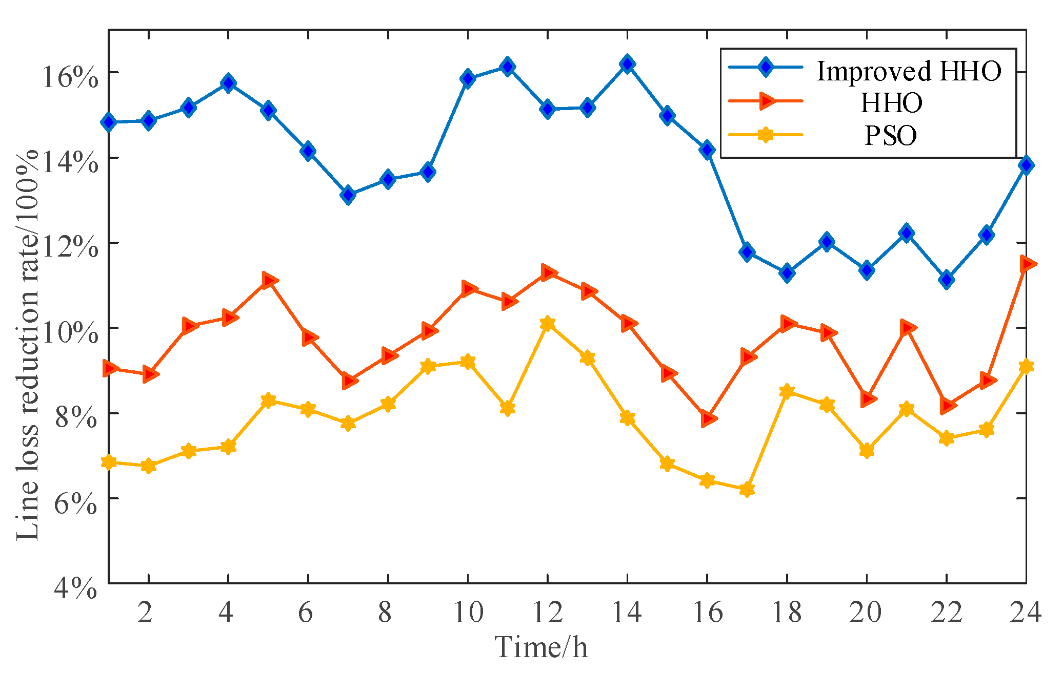
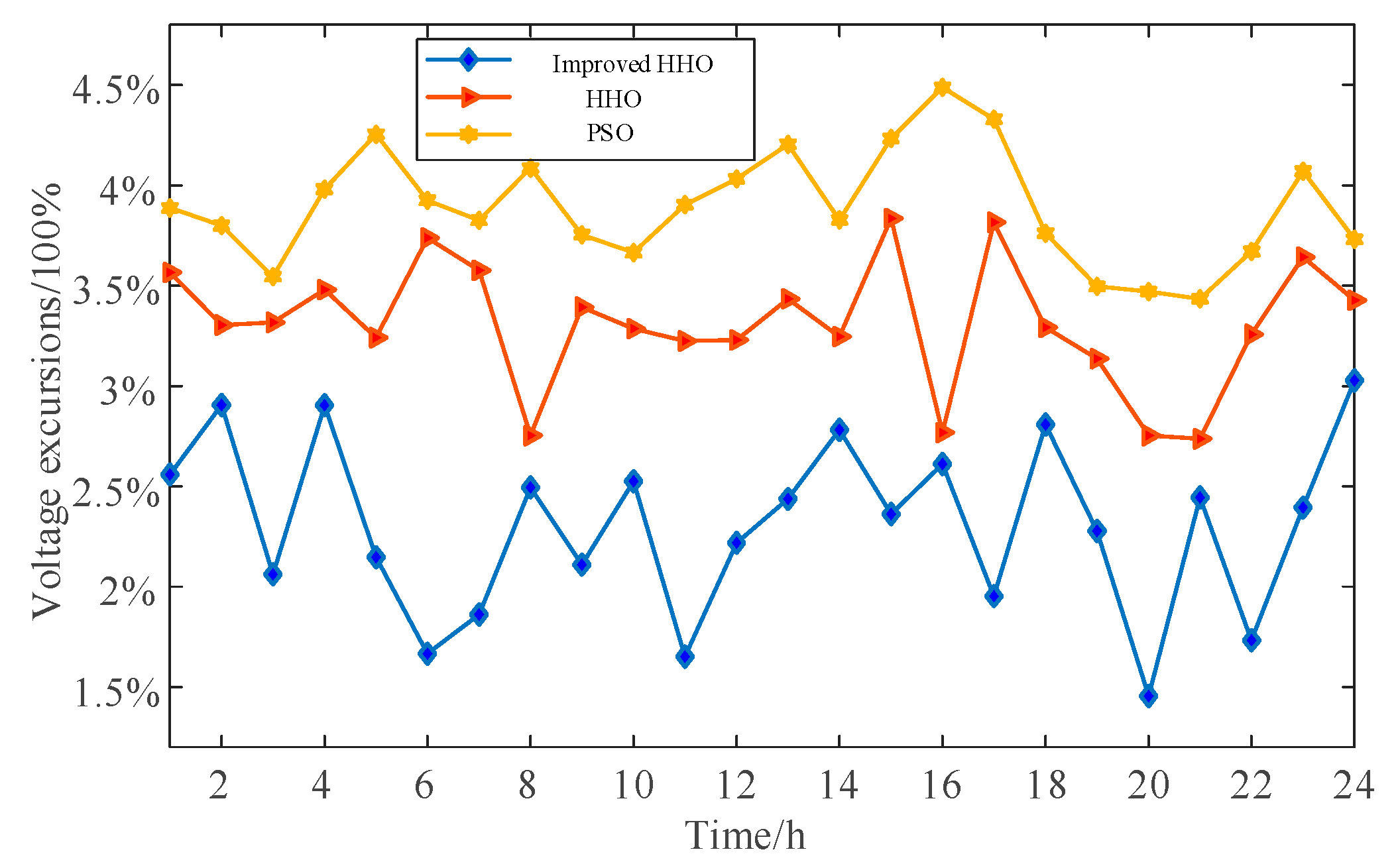
After applying the comprehensive reactive power optimisation strategy derived from the conventional HHO algorithm, the average system loss reduction rate is 9.75%, and the average voltage deviation is 3.311%.
(2)
After applying the integrated reactive power optimisation strategy derived from the particle swarm optimisation algorithm, the average system loss reduction rate is 8.16%, and the average voltage deviation is 3.962%.
(3)
After applying the integrated reactive power optimisation strategy derived from the multi-strategy improved HHO algorithm, the average system loss reduction rate is 13.90%, and the average voltage deviation is 2.308%.
By comparing the integrated reactive power strategies derived from the three algorithms, the overall effect of the unimproved traditional HHO algorithm is shown to be better than the particle swarm optimisation algorithm at reducing the system voltage deviation and line loss, while the voltage deviation and line loss of the system at all moments of the optimised system recorded using the improved HHO algorithm of the multi-strategy HHO algorithm is significantly better than that of the traditional HHO algorithm, which confirms the superiority of the multi-strategy HHO algorithm with regard to solving the model of the reactive power optimisation strategy proposed in this paper.

6. Conclusions

In this paper, the method of constructing a comprehensive reactive power optimisation strategy for power grids containing large-scale wind power based on the improved HHO algorithm was analysed, and the following conclusions were obtained:
(1)
The system voltage weak nodes were identified as reactive power compensation nodes based on the continuous tidal current method and the node voltage change index, which avoided the optimisation process of the access location of the reactive power compensation equipment, reduced the variable dimensions of the integrated reactive power optimisation model, and facilitated the construction and solution of the integrated reactive power optimisation model.
(2)
By analysing the reactive power regulation capability of wind farms, the reactive power potential of wind farms was fully explored, meaning that they could participate in the reactive power optimisation of the system, which could reduce the input of reactive power compensation equipment and improve the economy while increasing the energy utilisation of wind farms.
(3)
The traditional HHO algorithm was improved using the Harris Hawk population Corsi change, prey jumping strength optimisation and prey position adaptive weighting, and the improved algorithm had a performance superior to that of the traditional HHO algorithm and particle swarm optimisation algorithm when solving the comprehensive reactive power optimisation model proposed in this paper.

Author Contributions

Methodology, J.Z.; Validation, M.Z.; Formal analysis, C.W.; Investigation, B.Z., X.D. and L.S.; Writing—original draft, H.Z. All authors have read and agreed to the published version of the manuscript.

Funding

This work was supported by the Science and Technology Project of China Yunnan Power Grid Corporation (YPGC) (Project Number: YNKJXM20222105).

Institutional Review Board Statement

Not applicable.

Informed Consent Statement

Not applicable.

Data Availability Statement

No new data were created during the study period.

Conflicts of Interest

The authors declare that they have no known competing financial interest or personal relationships that could have appeared to influence the work reported in this paper.

References

  1. Shu, Y.B.; Chen, G.P.; He, J.B.; Zhang, F. Study on the framework of building a new power system with new energy as the main source. Strateg. Study CAE 2021, 23, 61–69. [Google Scholar] [CrossRef]
  2. Wang, X.; Wang, L.; Kang, W.; Li, T.; Zhou, H.; Hu, X.; Sun, K. Distributed Nodal Voltage Regulation Method for Low-Voltage Distribution Networks by Sharing PV System Reactive Power. Energies 2023, 16, 357. [Google Scholar] [CrossRef]
  3. Guo, P.; Chen, B.; Gao, Y.C.; Chen, Y.H.; Liu, L.; Peng, X.T. A generator reactive power optimisation method based on XGBOOST-PSO to improve the transient stability of the voltage at the receiving end grid. Power Syst. Prot. Control 2023, 51, 148–158. [Google Scholar]
  4. Xue, L.; Niu, T.; Fang, S.D.; Chen, G.H. A master-slave cooperative dynamic reactive power optimisation method taking into account the transient voltage safety of high percentage wind power. Autom. Electr. Power Syst. 2023, 1–15. [Google Scholar]
  5. Jiang, Z.J.; Yuan, X.; Qiu, W.H.; Huang, L.C.; He, W. Active distribution network reactive power optimisation model containing new energy and electric vehicle charging stations connected to the grid. Proc. CSU-EPSA 2023, 1–11. [Google Scholar]
  6. Lu, J.; Chang, J.X.; Zhang, Y.G.; E, S.P.; Zeng, C.H. Two-stage reactive power chance-constrained optimization method for an active distribution network considering DG uncertainties. Power Syst. Prot. Control. 2021, 49, 28–35. [Google Scholar]
  7. Xiao, H.; Pei, W.; Dong, Z.M.; Pu, T.J.; Chen, N.S.; Kong, L. Reactive power optimization of distribution network with distributed generation using metamodel-based global optimization method. Proc. CSEE 2018, 38, 1–13. [Google Scholar]
  8. Lin, S.H.; Wu, J.K.; Mo, C.; Wang, Z.Q.; Guo, Q.Y. Dynamic partition and optimization method for reactive power of distribution networks with distributed generation based on second-order cone programming. Power Syst. Technol. 2018, 42, 238–246. [Google Scholar]
  9. Yao, L.N.; Li, Q.H.; Yang, J.X.; Zhang, Y.J. Comprehensive reactive power optimization of power distribution and consumption system with support of electric vehicle charging and discharging. Autom. Electr. Power Syst. 2021, 46, 39–47. [Google Scholar]
  10. Ruan, H.B.; Gao, H.J.; Liu, J.Y.; Huang, Z. A distributionally robust reactive power optimization model for active distribution network considering reactive power support of DG and switch reconfiguration. Proc. CSEE 2019, 39, 685–695. [Google Scholar]
  11. Wu, G.; Wang, W.; Zhang, Y.; Yi, Y.; Zeng, S. Time decoupled dynamic extended reactive power optimization in incremental distribution network with photovoltaic-energy storage hybrid system. Power Syst. Prot. Control 2019, 47, 173–179. [Google Scholar]
  12. Chen, Q.; Wang, W.Q.; Wang, H.Y.; Wu, J.H. Research on dynamic reactive power compensation optimization strategy for distribution networks with distributed generation. Acta Energiae Solaris Sin. 2023, 44, 525–535. [Google Scholar]
  13. Wang, Z.Q.; Chen, J.F.; Zhang, G.F.; Yang, Q.; Dai, Y.H. Optimal power flow calculation with moth-flame optimization algorithm. Power Syst. Technol. 2017, 41, 3641–3647. [Google Scholar]
  14. Su, X.J.; Peng, H.; Mi, Y.; Fu, Y. Real-time optimization of voltage and reactive power in low- and medium-voltage unbalanced distribution networks based on linear programming. Power Syst. Technol. 2022, 1–14. [Google Scholar]
  15. Zhang, J.; Zheng, Y.Y.; Liu, S.C.; Ma, Y.F.; Yan, W. Dynamic reactive power optimization algorithm for regional power grids based on decoupled interior point method and mixed integer programming method. Electr. Power 2023, 56, 112–118. [Google Scholar]
  16. Zhou, B.X.; Yang, J.J.; Liu, Z.F.; Liu, S.C. Two-stage dynamic reactive power optimization for power systems based on improved state transfer algorithm. Power Capacit. React. Power Compens. 2021, 42, 22–30. [Google Scholar]
  17. Sun, T.; Zou, P.; Yang, Z.F.; Zhong, H.W.; Dai, G.H. A multi-stage solution method for dynamic reactive power optimization. Power Syst. Technol. 2016, 40, 1804–1810. [Google Scholar]
  18. Xiao, J.H.; Li, C.L.; Huang, X.Q.; Chen, D.P.; Ou, Z. Research on reactive power optimization of distribution networks containing wind power based on particle swarm algorithm. Electr. Eng. 2022, 18, 133–134+139. [Google Scholar]
  19. Xia, Z.L.; Lu, L.S.; Wu, Q.F.; Li, C.; Chen, Y. Application of improved grey wolf algorithm in reactive power optimisation of distribution network containing wind power. Smart Power 2023, 51, 63–70. [Google Scholar]
  20. Chen, Q.; Wang, W.Q.; Wang, H.Y. Strategy for optimal operation of a two-tier distribution grid containing distributed energy sources. Acta Energiae Solaris Sin. 2022, 43, 507–517. [Google Scholar]
  21. Wang, G.; Wu, X.; Li, L.; Zhang, M.Y.; Li, X.Z.; Chen, K.; Zhang, J.X. Optimization method of reactive power and harmonics under different output states of PV multifunctional grid-connected inverters. Electr. Power Autom. Equip. 2023, 1–12. [Google Scholar]
  22. Chen, L. Research on Several Issues of Distributed Generation Connecting to Power System; Zhejiang University: Hangzhou, China, 2007. [Google Scholar]
  23. Jin, J.L.; Li, X.T.; Liang, H.; Zhang, Y.L.; Peng, S.T.; Zuo, B.F.; Xu, J.; Zhan, J.Q. Calculation method of voltage stability limit based on improved continuous power flow method. Smart Power 2021, 49, 46–50. [Google Scholar]
  24. Cao, J.; Dang, Y. Fast calculation method of static voltage stability limit point of wind power connection system. Electr. Autom. 2020, 42, 13–16. [Google Scholar]
  25. Yang, L.; Wu, C.; Huang, W.; Guo, C.; Xiang, C. Multi-objective reactive power optimisation algorithm for new energy grid with high proportion of wind and solar energy. Electr. Power Constr. 2020, 41, 100–109. [Google Scholar]
  26. Liu, H.Z.; Li, Y.G.; Wang, Y.Y.; Zhang, X.T.; Cao, N.J. Impact of reactive voltage optimisation on new energy consumption. Transac. China Electr. Society 2019, 34, 646–653. [Google Scholar]
  27. Wang, Y.X.; Dai, C.B.; Yang, Z.C.; Xu, G.Y.; Bi, T.S. Wind farm reactive voltage control strategy considering wind turbine reactive potential. Power Syst. Prot. Control 2022, 50, 83–90. [Google Scholar]
  28. Heidari, A.A.; Mirjalili, S.; Faris, H.; Aljarah, I.; Mafarja, M.; Chen, H. Harris hawks optimization: Algorithm and applications. Future Gener. Comput. Syst. 2019, 97, 849–872. [Google Scholar] [CrossRef]
  29. Jingwei, T.; Abdul, R. A new quadratic binary harris hawk optimization for feature selection. Electronics 2019, 8, 1130–1156. [Google Scholar]
  30. Jia, H.M.; Lang, C.B.; Oliva, D.; Song, W.L.; Peng, X.X. Dynamic harris hawks optimization with mutation mechanism for satellite image segmentation. Remote Sens. 2019, 11, 1421. [Google Scholar] [CrossRef]
Figure 1. Flow chart to solve the integrated reactive power optimisation strategy.
Sustainability 15 12962 g001
Figure 2. Doubly fed asynchronous wind turbine power transfer and conversion model.
Sustainability 15 12962 g002
Figure 3. Iterative adaptive decay of prey escape energy.
Sustainability 15 12962 g003
Figure 4. Prey jump intensity real-time iterative processing.
Sustainability 15 12962 g004
Figure 5. Flow chart for solving a comprehensive reactive power optimisation strategy based on the improved HHO algorithm.
Sustainability 15 12962 g005
Figure 6. New energy wind-load improved IEEE-30 node system.
Sustainability 15 12962 g006
Figure 7. Node voltage variation index after wind farm access.
Sustainability 15 12962 g007
Figure 8. PV curves of weak nodes of the simulation sample voltage on the day of optimisation.
Sustainability 15 12962 g008
Figure 9. Convergence curves of the objective function fitness values obtained using different algorithms.
Sustainability 15 12962 g009
Figure 10. Optimised system line loss reduction rate.
Sustainability 15 12962 g010
Figure 11. Optimised system voltage excursions.
Sustainability 15 12962 g011
Table 1. 24-h reactive power regulation range for wind farms.
Time/h v w /(m/s) P g /(MW) P c /(MW) P s /(MW) Q g /(Mvar)
1:008.7285.3340.0935.428[−6.952, 8.378]
2:0015.79212.0210.21012.232[−9.595, 11.157]
3:003.4470.9940.0171.011[−5.251, 6.577]
4:008.2094.9930.0875.080[−6.819, 8.237]
5:008.8835.4330.0955.528[−6.991, 8.419]
6:0014.4779.4950.1669.661[−8.612, 10.107]
7:0012.5087.8030.1377.940[−7.931, 9.401]
8:005.0772.6260.0462.672[−5.897, 7.259]
9:0015.95713.5240.23713.761[−10.163, 11.783]
10:008.8675.4200.0955.515[−6.987, 8.415]
11:009.0225.5200.0975.617[−7.027, 8.456]
12:0015.91012.8030.22413.027[−9.891, 11.482]
13:0015.93913.1630.23013.394[−10.027, 11.633]
14:0015.94113.2030.23113.434[−10.042, 11.650]
15:004.6192.2050.0392.244[−5.731, 7.085]
16:005.7853.2270.0563.283[−6.131, 7.508]
17:006.4483.7480.0663.813[−6.334, 7.723]
18:0016.00416.870.29517.165[−11.486, 13.169]
19:007.7044.6490.0814.730[−6.686, 8.096]
20:0014.4599.4770.1669.643[−8.604, 10.099]
21:009.7125.9610.1046.065[−7.200, 8.639]
22:006.6893.9250.0693.994[−6.404, 7.798]
23:0014.7169.7770.1719.948[−8.723, 10.224]
24:008.0444.8850.0854.970[−6.776, 8.192]
Table 2. Comparison between line loss results obtained using different algorithms.
Time/hLine Loss/MWLoss Reduction Rate
UnoptimisedPSOHHOImproved HHOPSOHHOImproved HHO
1:0019.07617.76917.34916.2476.85%9.05%14.83%
2:0019.15917.86417.45216.3126.76%8.91%14.86%
3:0019.37918.00117.43316.4397.11%10.04%15.17%
4:0019.20617.82117.23916.1817.21%10.24%15.75%
5:0019.03317.45316.91816.1588.30%11.11%15.10%
6:0019.19917.64617.32216.4838.09%9.78%14.15%
7:0019.06717.58717.39716.5667.76%8.76%13.12%
8:0018.82717.28117.06816.2888.21%9.34%13.48%
9:0018.89017.17117.01416.3099.10%9.93%13.66%
10:0018.93617.19216.86815.9349.21%10.92%15.85%
11:0019.02317.48017.00315.9548.11%10.62%16.13%
12:0019.09317.16516.93616.20410.10%11.30%15.13%
13:0019.13117.35217.05316.2299.30%10.86%15.17%
14:0018.95617.46017.04015.8877.89%10.11%16.19%
15:0019.68218.34217.92316.7336.81%8.94%14.98%
16:0018.63817.44117.17115.9966.42%7.87%14.18%
17:0019.13317.94517.35016.8796.21%9.32%11.78%
18:0018.84417.24016.94116.7178.51%10.10%11.29%
19:0019.07517.51117.18916.7828.20%9.89%12.02%
20:0018.82517.48517.25616.6887.12%8.34%11.35%
21:0018.57817.07316.72016.3078.10%10.00%12.23%
22:0019.09817.68317.53616.9727.41%8.18%11.13%
23:0018.95617.51317.29416.6477.61%8.77%12.18%
24:0019.04917.31616.85816.4179.10%11.50%13.82%
Table 3. Comparison between voltage offset results obtained using different algorithms.
Time/hVoltage Excursions (%)Time/hVoltage Excursions (%)
UnoptimisedPSOHHOImproved HHOUnoptimisedPSOHHOImproved HHO
1:006.013.893.572.5613:006.064.213.442.437
2:006.083.803.302.9114:006.103.833.252.782
3:006.033.553.322.0615:006.024.233.842.362
4:006.093.983.482.9116:006.064.492.772.611
5:006.034.263.242.1517:006.074.333.821.953
6:006.053.933.741.6718:006.043.763.292.807
7:006.083.833.581.8619:006.013.493.142.277
8:006.064.072.752.4920:006.063.472.751.455
9:006.093.753.392.1121:006.033.442.742.444
10:006.033.673.292.5322:005.993.673.261.733
11:006.053.903.221.6523:006.044.073.642.394
12:006.084.033.232.2224:006.173.733.433.027
Disclaimer/Publisher’s Note: The statements, opinions and data contained in all publications are solely those of the individual author(s) and contributor(s) and not of MDPI and/or the editor(s). MDPI and/or the editor(s) disclaim responsibility for any injury to people or property resulting from any ideas, methods, instructions or products referred to in the content.

