An Intelligent Algorithm for Solving Unit Commitments Based on Deep Reinforcement Learning

Abstract

With the reform of energy structures, the high proportion of volatile new energy access makes the existing unit commitment (UC) theory unable to satisfy the development demands of day-ahead market decision-making in the new power system. Therefore, this paper proposes an intelligent algorithm for solving UC, based on deep reinforcement learning (DRL) technology. Firstly, the DRL algorithm is used to model the Markov decision process of the UC problem, and the corresponding state space, transfer function, action space and reward function are proposed. Then, the policy gradient (PG) algorithm is used to solve the problem. On this basis, Lambda iteration is used to solve the output scheme of the unit in the start–stop state, and finally a DRL-based UC intelligent solution algorithm is proposed. The applicability and effectiveness of this method are verified based on simulation examples.

1. Introduction

The unit commitment (UC) problem is the core link and theoretical basis of day-ahead generation scheduling and day-ahead market trading in power systems [1]. In the day-ahead operation of the electricity market, one of the most critical processes is to determine a unit scheduling scheme subject to various constraints [2]. Therefore, it is of great theoretical and practical significance to study a solution method for security-constrained unit commitment (SCUC) with high accuracy, applicability and efficiency.

The current research on SCUC is mainly divided into two categories. The first type is a physical model-driven version of the traditional SCUC decision-making method (PMD-SCUC). That is to say, starting from the specific practical engineering problems [3], the corresponding mathematical model is constructed. Then, the corresponding theory or method is used to simplify and process the model [4,5]. On this basis, the solution algorithm for the model is studied [6]. Although this idea allows good physical interpretation, the modeling and solving processes of this idea are very complex. In practical applications, in order to improve the efficiency of solving, the model and solving algorithm are often simplified appropriately, which leads to a decline in the decision-making accuracy of the model [7]. Moreover, when specific problems and application scenarios change, the previously constructed model and the adopted solution algorithm must be improved and changed accordingly, and the applicability is low in the new power system, with various theoretical problems and engineering needs constantly emerging.

In contrast, the SCUC decision-making method based on machine learning (ML) is a more effective way of thinking [8]. Differently from the PMD decision-making method, this method does not study the internal mechanisms of unit commitment, but directly constructs the mapping relationships between known inputs and decision results based on in-depth learning methods and massive historical decision data training [9]. This method can not only greatly simplify the process and complexity of modeling, and solve the unit commitment problem, but also cope with various emerging theoretical problems and challenges through its self-learning and self-evolution processes [10]. Reference [11] proposes a two-order data-driven (DD) SCUC model, which is founded on a nonparametric Dirichlet-process Gaussian mixture model and a variational Bayesian inference method, to describe the uncertainties of load, PV and wind power. Reference [12] proposes a modeling method of a generalized convex hull uncertainty set based on DD, and applies the uncertainty set to a two-stage robust UC. Although the related algorithms of ML are mentioned in the above studies, the traditional mathematical optimization method is still used to solve the SCUC model. A purely DD-based SCUC decision method is first presented in reference [13]. This method does not study the internal mechanisms of UC, but constructs a deep learning (DL) model based on long short-term memory (LSTM), and directly constructs a mapping model between system load and dispatching decision results through historical data training, which provides a new solution idea for the study of SCUC. However, the existing ML-based SCUC decision methods belong to supervised learning, which often requires massive high-quality sample data for training [14]. In many scenarios, however, people often cannot guarantee accumulating massive high-quality historical decision data, which limits the applicability of such methods.

Reinforcement learning (RL) can effectively find the optimal strategy [15] in the complex control field through trial and error. At present, RL has also been explored and applied in the field of power systems, such as using remedial measures to maintain system safety [16], controlling the load frequency of motors [17], controlling the transient stability of power systems [18], ensuring optimal bidding of generators [19], etc. Its biggest feature is that it completely jumps out of the inherent mode of supervised learning, does not need to process a large amount of label data in advance, and has high generalization performance [20]. In addition, DL can analyze environmental information and extract features from it [21], avoiding the difficulty of storing Q value tables in RL in large data application scenarios [22].

In view of this, this paper proposes a UC intelligent solution algorithm combined with deep reinforcement learning (DRL) technology. Firstly, the DRL algorithm is introduced to model the UC problem with the Markov decision process (MDP), and the corresponding state space, transition function, action space and reward function are given. Then, the policy gradient (PG) algorithm is used to solve it. On this basis, lambda iteration is used to solve the output scheme of the unit in the start–stop state and, finally, an intelligent algorithm for solving UC based on DRL is proposed. The applicability and effectiveness of the proposed method are verified via simulations based on standard examples.

The main contributions of this paper are as follows.

The proposed intelligent algorithm for solving UC problems based on DRL can effectively make decisions for complex small-scale UC problems. Compared with supervised learning, the method does not need to construct a large amount of labeled sample data in advance, avoids dependence on the sample data, and has a higher generalization performance. Moreover, it can directly give the action decision through the strategy model, and the solving efficiency is high.

2. DRL-Based Algorithm Architecture for Unit Commitment

In this paper, DRL is applied to the field of UC decisions [23], and an intelligent algorithm for solving UC based on DRL is proposed. The UC problem is calculated in two steps, and the decision block diagram is shown in Figure 1.

The first step is to decide the current unit start–stop scheme based on DRL. The second step is to solve the economic dispatching problem based on Lambda iteration according to the start–stop scheme of the unit at the current time. In the first step, the DRL algorithm is used to establish the MDP model of the UC problem. Based on the characteristics of the UC problem, the state space, action space, transfer function and reward function are given, the PG algorithm is used to solve the problem, and the optimal unit action mode at the current time is obtained. In the second step, Lambda iteration is adopted to solve the economic dispatching problem according to the unit start–stop mode obtained in the first step, and the specific output value of the unit at that moment is obtained. Therefore, the system operation cost at the current moment is obtained accordingly.

3. Solution of Unit Startup and Shutdown Scheme Based on DRL

3.1. Mathematical Model of Unit Commitment

(1)

Objective function

The optimization objective of the SCUC problem is to minimize the total operation cost of the system on the premise of ensuring the safe and stable operation of the power system [24]. The cost consists of the start-up cost and operation cost of the thermal power-generating unit. The objective function is as follows:

$$F^{G,\cos t}(U_{{\beta }^{TP}t}^{G,\mathrm{S}\mathrm{T}},P_{{\beta }^{TP}t}^{G,AP})=\min {\displaystyle \sum _{t=1}^T{\displaystyle \sum _{{\beta }^{TP}=1}^{N^{TP}}\left[U_{{\beta }^{TP}t}^{G,\mathrm{S}\mathrm{T}}\left(1-U_{{\beta }^{TP}\left(t-1\right)}^{G,\mathrm{S}\mathrm{T}}\right)F^{G,SU,\cos t}+U_{{\beta }^{TP}t}^{G,\mathrm{S}\mathrm{T}}{F}^{G,RU,\cos t}\left(P_{{\beta }^{TP}t}^{G,AP}\right)\right]}}$$

(1)

The specific expressions of start-up cost and operation cost are as follows:

$$F^{G,SU,\cos t}={\alpha }_{{\beta }^{TP},1}^{SU}+{\alpha }_{{\beta }^{TP},2}^{SU}(1-e^{{\tau }_{{\beta }^{TP}t}^G/{\xi }_{{\beta }^{TP}}})$$

(2)

$$F^{G,RU,\cos t}(P_{{\beta }^{TP}t}^{G,AP})=a_{{\beta }^{TP},1}^{RU}+a_{{\beta }^{TP},2}^{RU}{P}_{{\beta }^{TP}t}^{G,AP}+a_{{\beta }^{TP},3}^{RU}{(P_{{\beta }^{TP}t}^{G,AP})}^2$$

(3)

where $U_{{\beta }^{TP}t}^{G,\mathrm{S}\mathrm{T}}$ indicates the startup and shutdown status of the thermal power unit, ${\beta }^{TP}$, at time t; $P_{{\beta }^{TP}t}^{G,AP}$ is the active power output of the thermal power unit, ${\beta }^{TP}$, at time t; $N^{TP}$ indicates the total number of thermal power units participating in dispatching; $T$ indicates the dispatching period; ${\alpha }_{{\beta }^{TP},1}^{SU}$ represents the startup cost of the thermal power unit, ${\beta }^{TP}$; ${\alpha }_{{\beta }^{TP},2}^{SU}$ represents the startup cost of the thermal power unit, ${\beta }^{TP}$, under cold conditions; ${\tau }_{{\beta }^{TP}t}^G$ indicates the continuous shutdown time of thermal power unit, ${\beta }^{TP}$, at time t; ${\zeta }_{{\beta }^{TP}}$ is the time constant of the cooling rate of the thermal power-generating unit, ${\beta }^{TP}$; $a_{{\beta }^{TP},1}^{RU}$, $a_{{\beta }^{TP},2}^{RU}$, and $a_{{\beta }^{TP},3}^{RU}$ are the operating cost parameters of the thermal power-generating unit, ${\beta }^{TP}$.

(2)

Constraints

The constraint conditions include the system constraints required in the normal operation of the power system and the inherent physical constraints of the generating units [25]. The former include power flow security constraints and power balance constraints, while the latter include unit active power output constraints, ramp constraints, minimum start–stop time constraints, maximum start–stop time constraints and spinning reserve capacity constraints. The specific description is as follows:

(a)

Power balance constraint

Since electric energy cannot be stored on a large scale, it is required that in addition to meeting the unit’s own power consumption and line loss, the supply and demand sides should maintain a balance in real time [26]. As long as there is a power imbalance, the frequency or voltage of the system will fluctuate. When the fluctuation exceeds the maximum range allowed by the power grid, there will be serious accidents such as equipment damage and even power grid disconnection [27]. Therefore, it is required to keep real-time balance between the total power generation and the total load demand of all units in the system, and its mathematical expression is as follows:

$${\displaystyle \sum _{{\beta }^{TP}=1}^{N^{TP}}{P}_{{\beta }^{TP}t}^{G,AP}+}{P}_{Wt}=P_t^{L,AP}$$

(4)

where $P_t^{L,AP}$ represents the total load of the system at time t; $P_{Wt}$ represents the output power of the wind turbine generator system at time t.

(b)

Unit operation constraints

Due to the limitations of the physical characteristics of the unit itself, when the unit works normally, its output can only be limited to a certain range, and its mathematical expression is as follows:

$$P_{{\beta }^{TP}\min }^{G,AP}\le P_{{\beta }^{TP}t}^{G,AP}\le P_{{\beta }^{TP}\max }^{G,AP}$$

(5)

where $P_{{\beta }^{TP}\max }^{G,AP}$ and $P_{{\beta }^{TP}\min }^{G,AP}$ represent the upper and lower limits of thermal power unit output, respectively.

(c)

Unit climbing constraint

Climbing constraint refers to the constraint restriction on the increase and decrease in output of the unit [28]. However, when the output value of the unit needs to be adjusted due to factors such as load change [29], it cannot be adjusted to the required output value immediately due to the limitations of the physical characteristics of the unit itself. Its mathematical expression is as follows:

$$\mathsf{\Delta }{P}_{{\beta }^{TP}}^{G,\mathrm{U}\mathrm{P}}{U}_{{\beta }^{TP}t}^{G,ST}+P_{{\beta }^{TP}\min }^{G,AP}(U_{{\beta }^{TP}t}^{G,ST}-U_{{\beta }^{TP}(t-1)}^{G,ST})\ge P_{{\beta }^{TP}t}^{G,AP}-P_{{\beta }^{TP}(t-1)}^{G,AP}$$

(6)

$$\mathsf{\Delta }{P}_{{\beta }^{TP}}^{G,\mathrm{D}\mathrm{O}\mathrm{W}\mathrm{N}}{U}_{{\beta }^{TP}(t-1)}^{G,ST}+P_{{\beta }^{TP}\min }^{G,AP}(U_{{\beta }^{TP}(t-1)}^{G,ST}-U_{{\beta }^{TP}t}^{G,ST})\ge P_{{\beta }^{TP}(t-1)}^{G,AP}-P_{{\beta }^{TP}t}^{G,AP}$$

(7)

where $\mathsf{\Delta }{P}_{{\beta }^{TP}}^{G,\mathrm{U}\mathrm{P}}$ and $\mathsf{\Delta }{P}_{{\beta }^{TP}}^{G,\mathrm{D}\mathrm{O}\mathrm{W}\mathrm{N}}$ respectively represent the climbing up and climbing down constraints of the thermal power-generating unit.

(d)

Minimum start–stop time constraint

When the unit is in the shutdown state, there is a minimum continuous downtime constraint before it changes to being in the startup state. Similarly, there is a minimum continuous boot time constraint.

$$\left\{\begin{array}{c}(A_{{\beta }^{TP}(t-1)}^{G,UP}-T_{{\beta }^{TP}}^{G,UP})(U_{{\beta }^{TP}(t-1)}^{G,ST}-U_{{\beta }^{TP}t}^{G,ST})\ge 0\\ (A_{{\beta }^{TP}(t-1)}^{G,DOWN}-T_{{\beta }^{TP}}^{G,DOWN})(U_{{\beta }^{TP}t}^{G,ST}-U_{{\beta }^{TP}(t-1)}^{G,\mathrm{S}\mathrm{T}})\ge 0\end{array}\right.$$

(8)

where $A_{{\beta }^{TP}(t-1)}^{G,\mathrm{U}\mathrm{P}}$ and $A_{{\beta }^{TP}(t-1)}^{G,\mathrm{D}\mathrm{O}\mathrm{W}\mathrm{N}}$ respectively represent the continuous startup and shutdown time of the thermal power unit, ${\beta }^{TP}$; $T_{{\beta }^{TP}}^{G,\mathrm{U}\mathrm{P}}$ and $T_{{\beta }^{TP}}^{G,\mathrm{D}\mathrm{O}\mathrm{W}\mathrm{N}}$ respectively represent the minimum continuous startup and shutdown time of the thermal power unit, ${\beta }^{TP}$.

(e)

Maximum start–stop time constraint

The maximum start–stop time constraint means that in the actual operation of the unit, its frequent start–stop adjustment will produce mechanical losses, thereby shortening the normal working time of the thermal power unit, and thus affecting the normal operation of the power system [30]. Based on this, it is necessary to limit the maximum number of startups and shutdowns of thermal power units in the dispatching cycle. The mathematical expression is as follows:

$${\displaystyle \sum _{t=1}^T|U_{{\beta }^{TP}t}^{G,ST}-U_{{\beta }^{TP}(t-1)}^{G,ST}|}\le {\chi }_{{\beta }^{TP}}$$

(9)

where ${\chi }_{{\beta }^{TP}}$ refers to the maximum allowable times of startup and shutdown of the thermal power-generating unit, ${\beta }^{TP}$, in the dispatching period.

(f)

Maximum start–stop time constraint

$${\displaystyle \sum _{{\beta }^{TP}=1}^{N^{TP}}{P}_{{\beta }^{TP}t}^{G,AP}=P_t^{L,AP}}$$

(10)

3.2. MDP Modeling for Unit Commitment

MDP is composed of the state space, reward function, action space, and transition function. The objective of the UC problem studied in this paper is to maximize the reward by minimizing the total running cost of the system [31].

(1)

State space

In this MDP, it is hoped that the model can provide the start–stop state of the unit at each moment according to the given input data. Therefore, the input data at each moment constitute the state space. Specifically, the state space includes the start–stop time and load demand data of the N generating units. Its mathematical expression is as follows:

$$S=\{U_t,P_L\}$$

(11)

where $U_t=[u_{1,t},u_{2,t},\dots u_{N,t}]$, in which $u_{i,t}\ne 0$, represents the set of the unit start–stop time; $P_L$ represents the load demand data. Since the objective of the UC problem is to solve the unit scheduling plan with the lowest total cost according to the given load demand under the condition of meeting various constraints, this variable has a very important impact on this problem [32].

(2)

Action space

In RL, the action space is required to be complete, efficient, and legal. (a) Completeness refers to ensuring that the action space contains all actions that can complete the target task. In this problem, the goal is to find the start–stop states of the units, so the action space should contain the start–stop states of all units. (b) In terms of high efficiency, in the decision variables of this optimization problem, both discrete variables and continuous variables are involved, so it is difficult to solve them [33]. Based on this, the unit start–stop scheme and the unit output scheme are solved step by step in this paper. After the UC solution algorithm based on DRL is used to obtain the unit start–stop scheme, Lambda iteration is used to solve the unit output scheme. (c) Legitimacy means that the actions in the action space are required to meet various constraints.

At any time, the possible action of each unit is to start or to stop. Therefore, the action space is the combination of all unit start or stop actions, and the size of the action space is $2^N$. Represent it as a binary array; that is,

$$A_t=[a_{1,t},a_{2,t},\dots a_{N,t}]$$

(12)

When the action of the unit is to start, $a_{i,t}=1$. When the action of the unit is to stop, $a_{i,t}=0$. However, this action must comply with the minimum startup–shutdown time constraints of the unit.

(3)

Transfer function

When the model decides the unit startup and shutdown scheme according to the observed state information and obtains the reward value, the transition function will change from state $s_t$ to state $s_{t+1}$ according to the unit startup and shutdown action, $a_t$, under the condition of satisfying various constraints. The related state information in this paper is the continuous startup/shutdown time, $u_{i,t}$, of the unit. For the unit, $i$, the conversion function of its continuous startup/shutdown time is as follows:

$$u_{i,t+1}=\left\{\begin{array}{l}{u}_{i,t}+1, \mathrm{if} a_{i,t}=1 \mathrm{and} u_{i,t}>0\hfill \\ u_{i,t}-1, \mathrm{if} a_{i,t}=0 \mathrm{and} u_{i,t}<0\hfill \\ 1, \mathrm{if} a_{i,t}=1 \mathrm{and} u_{i,t}<0\hfill \\ -1, \mathrm{if} a_{i,t}=0 \mathrm{and} u_{i,t}>0\hfill \end{array}\right.$$

(13)

(4)

Reward function

The goal of RL is to maximize the reward obtained using the model on the path when solving the problem. In the problem studied in this paper, the goal is to minimize the total operating cost of the system. Therefore, the mathematical expression of its cost is as follows:

$$r_t=-(F_t+{\lambda }_t)$$

(14)

in which

$$F_t={\displaystyle \sum _{i=1}^N(a{P}_i{}^2+b{P}_i+c)+F_i{}^{up}}$$

(15)

where $F_t$ is the operation cost of the system at time t; $F_i{}^{up}$ is the start-up cost of the unit $i$; $P_i$ is the active power output value of the unit $i$; ${\lambda }_t$ is the penalty value for violating the operation constraint at time t.

In the MDP of UC, at each time t, the model observes the state information, $s_t$, in the power system, that is, the start/stop time and load demand data of N units at the current time. Then, the model chooses the optimal action, $a_t$, according to the state information, that is, the unit start–stop plan decided at the current time. Finally, according to the start–stop scheme, Lambda iteration is used to solve economic scheduling, and the actual output power of the unit at the current time is obtained. Based on this power, the operating cost of the system at the current moment is calculated, which is part of the reward function. After receiving the reward value, r, which evaluates the quality of the current unit startup and shutdown scheme, $a_t$, the model transfers to the next new state, $s_{t+1}$, and the transfer process is determined using formula (15). The specific solution process is shown in Figure 2.

As shown in Figure 2, the experience pool mechanism is introduced in the solution process, which mainly includes two processes of sample collection and sampling. The collected unit startup and shutdown status, load data, unit output scheme and reward value are put into the experience pool in order of time. When the experience pool is full, the sample data earlier in time are overwritten. When sampling, a batch of data will be randomly sampled uniformly from the experience pool for learning and updating.

The specific interaction process of MDP is as follows.

Define $G(t)$ as the reward value of the whole iterative process of the system, and multiply the reward value of the future moment by the discount to represent the importance of the future reward value [34,35]. Its mathematical expression is as follows:

$$G(t)=r_{t+1}+\gamma r_{t+2}+{\gamma }^2{r}_{t+3}+\dots ={\displaystyle \sum _{k=0}^{\infty }{\gamma }^k{r}_{t+k+1}}$$

(16)

where $\gamma \in [0,1]$ is the discount factor, which is used to control the relative weight of the immediate and future rewards. The larger the value is, the more important the reward value at the future time is; $r_t$ is the sum of the operating cost of the system at time t and the penalty for violating the constraints, and its expression is shown in formula (16).

In order to minimize the total operating cost of the system, the model needs to constantly update the existing unit startup and shutdown strategy, $\pi$, in the continuous interaction with the system environment, and finally obtains the optimal unit startup and shutdown strategy, ${\pi }^{\ast }$. To evaluate the degree of the current unit commitment scheme, $a_t$, given by the model under the current time step state information, the expectation function is usually used to quantify the objective function.

(5)

Policy gradient algorithm

The strategy-based PG algorithm has good convergence. Therefore, this paper uses this algorithm to solve the MDP model. The core idea of the PG algorithm is to parameterize the strategy for solving the unit start–stop scheme. The purpose of selecting the unit start–stop scheme with the minimum operating cost by controlling the weight of these parameters is to find the optimal commitment scheme by learning the gradient information of the strategy parameters. The specific unit startup and shutdown scheme strategy can be described as a function-containing parameter, $\theta$:

$${\pi }_{\theta }(s_t,a_t)=P(a_t|s_t,\theta )\approx \pi (s_t,a_t)$$

(17)

If the parameterized neural network is used to represent the unit startup and shutdown strategy, ${\pi }_{\theta }$, the objective function can be expressed as an adjusting parameter, $\theta$, to maximize the expected reward value, and its mathematical expression is as follows:

$$J_1(\theta )=V_{{\pi }_{\theta }}(s_1)=E_{{\pi }_{\theta }}(G_1)=E(r_1+\gamma r_2+{\gamma }^2{r}_3+\dots \dots |{\pi }_{\theta })$$

(18)

The objective function is maximized. That is, a set of parameter vectors, $\theta$, is searched such that the objective function is maximized. In general, for the maximization problem, a gradient ascent algorithm is used to find the maximum value:

$${\theta }^{\ast }=\theta +\alpha {\nabla }_{\theta }{J}_1(\theta )$$

(19)

Assume a MDP with only one step, and use the gradient ascent algorithm for it. ${\pi }_{\theta }(s_t,a_t)$ represents a function on the parameter, $\theta$, and the mapping is $P(a_t|s_t,\theta )$. The reward value of the unit start–stop scheme, $a_t$, obtained in the state, $s_t$, is $r_t=r(s_t,a_t)$. Then, the reward value obtained by selecting the unit start–stop scheme, $a_t$, is ${\pi }_{\theta }(s_t,a_t)r(s_t,a_t)$, and the weighted reward in the state, $s_t$, is ${\displaystyle {\sum }_{a\in A}{\pi }_{\theta }(s_t,a_t)r(s_t,a_t)}$, which is derived as follows:

$$J_1(\theta )=E_{{\pi }_{\theta }}[r(s_t,a_t)]={\displaystyle {\sum }_{s\in S}d(s){\displaystyle {\sum }_{a_t\in A}{\pi }_{\theta }(s_t,a_t)r(s_t,a_t)}}$$

(20)

The gradient is as follows:

$${\nabla }_{\theta }{J}_1(\theta )={\nabla }_{\theta }{\displaystyle {\sum }_{s\in S}d(s){\displaystyle {\sum }_{a_t\in A}{\pi }_{\theta }(s_t,a_t)r(s_t,a_t)}}={\displaystyle {\sum }_{s\in S}d(s){\displaystyle {\sum }_{a_t\in A}{\nabla }_{\theta }{\pi }_{\theta }(s_t,a_t)r(s_t,a_t)}}$$

(21)

where $d(s)$ represents the distribution of states in the strategy.

Assuming that the gradient ${\nabla }_{\theta }{\pi }_{\theta }(s,a)$ is known, the score function is defined as ${\nabla }_{\theta }\log {\pi }_{\theta }(s_t,a_t)$ by applying the likelihood ratio, and the relationship between them is as follows:

$${\nabla }_{\theta }{\pi }_{\theta }(s_t,a_t)={\pi }_{\theta }(s_t,a_t)\frac{{\nabla }_{\theta }{\pi }_{\theta }(s_t,a_t)}{{\pi }_{\theta }(s_t,a_t)}={\pi }_{\theta }(s_t,a_t){\nabla }_{\theta }\log {\pi }_{\theta }(s_t,a_t)$$

(22)

Therefore, formula (21) can be written as follows:

$${\nabla }_{\theta }{J}_1(\theta )={\displaystyle {\sum }_{s\in S}d(s)}{\displaystyle {\sum }_{a_t\in A}{\pi }_{\theta }(s_t,a_t)}{\nabla }_{\theta }\log {\pi }_{\theta }(s_t,a_t)r(s_t,a_t)$$

(23)

The policy gradient is restored to the desired form as follows:

$${\nabla }_{\theta }{J}_1(\theta )=E_{{\pi }_{\theta }}[{\nabla }_{\theta }\log {\pi }_{\theta }(s_t,a_t)r(s_t,a_t)]$$

(24)

By selecting the optimal unit start–stop scheme, $a_t$, to minimize the operation cost of the system, the following results are obtained:

$${\nabla }_{\theta }{J}_1(\theta )=E_{{\pi }_{\theta }}[{\nabla }_{\theta }\log {\pi }_{\theta }(s_t,a_t)R^{{\pi }_{\theta }}(s_t,a_t)]$$

(25)

The pseudocode of DRL for UC problems is summarized in Appendix B. Algorithm A1.

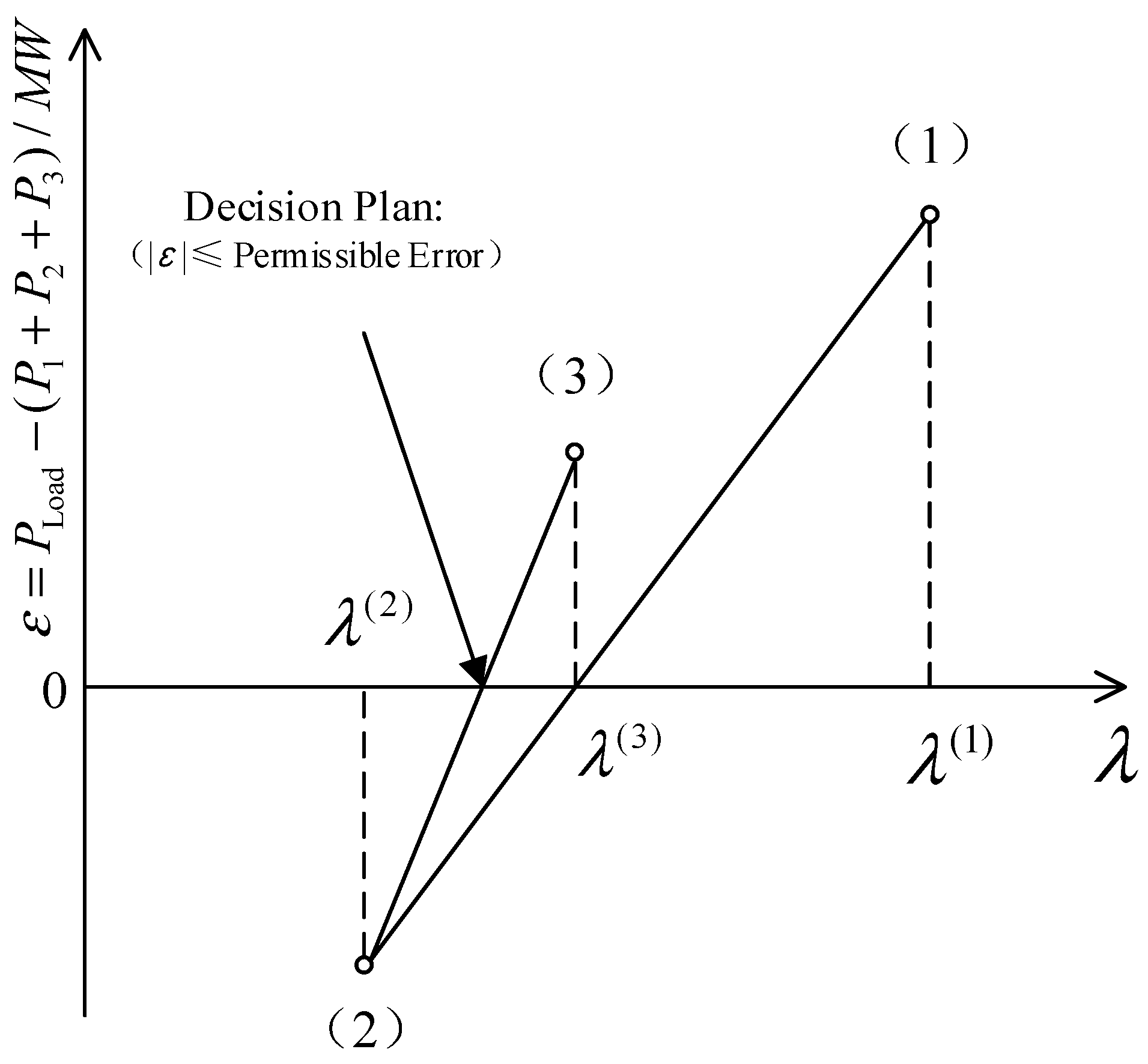
4. Solution of Unit Output Scheme Based on Lambda Iteration

Before the transition into the new state, the unit start–stop scheme, $a_t$, obtained using the solution is taken as the start–stop action of the unit in 24 h in the economic dispatching problem. According to the action, Lambda iteration is used to solve the problem, and the actual output power, $P$, of the unit in the startup state is given.

The Lambda iterative method is a classical algorithm in the field of economic dispatch. Its main principle is to make the cost incremental rate of all units equal and equal to the unknown parameter, $\lambda$. By calculating the difference between the total output value of the unit and the load demand to adjust $\lambda$, the active power output plan of all coal-fired units is finally obtained. The solution process is shown in Figure 3.

It is assumed that there is a system with three generating units, and it is hoped that the optimal economic operation point can be found. One way to carry this out is to characterize the incremental cost characteristics of each unit by plotting the incremental cost characteristics of the three units on the same graph, as shown in Figure 4.

In order to determine the optimal operating point for these three units, which minimizes the total cost while meeting the specified load demand, a solution can be found using a straight edge and a cost incremental rate characteristic chart of this unit. That is, a cost incremental rate value ($\lambda$) is given first, and the active output value of each of the three units is found according to this value.

In general, the $\lambda$ given for the first time is often inaccurate. If we assume a value of $\lambda$ that causes the total power output to be too low, we must increase the value of $\lambda$, which results in a new output power value. After obtaining these two sets of solutions, we can use the interpolation method shown in Figure 5 to further approach the expected value of the actual total output power.

By constantly tracking the corresponding relationship between $\lambda$ and the output power, the optimal economic operation point can be quickly solved. In addition, the total output power of all units corresponding to different values of $\lambda$ can be clearly seen through the table.

In this paper, according to flow chart of the block diagram shown in Figure 3, the personal computer (PC) is used for programming. By establishing a complete set of logical rules, it is possible to achieve the same purpose by using a cost incremental rate characteristic diagram and ruler.

In general, data tables can be stored in the PC and interpolated between the stored values to find the exact active output of the unit corresponding to $\lambda$.

In addition, the relationship between the unit output and $\lambda$ can be expressed in the form of an analytical function, which (or its coefficients) can be stored in PC, and then the output power of each unit can be determined using the function. In this paper, the second method is adopted.

The algorithm is an iterative algorithm. Therefore, a stopping rule must be established. Generally speaking, there are two common stopping rules for this iterative calculation. The first method is shown in Figure 3, which is to find the best economic operating point within the allowable error range. The second method is to set the maximum number of iterations, $\epsilon$, and stop the calculation when the number of iterations exceeds $\epsilon$. In this paper, the second method is adopted, and the maximum number of iterations is set to 50. For UC, a special type of optimization problem, the Lambda iterative method has a very fast convergence rate.

5. Example Simulation and Analysis

5.1. Explanation of Calculation Examples

In order to verify the correctness and effectiveness of the proposed method, a system with 10 thermal power units is simulated in this paper. The relevant parameters of 10 thermal power units are shown in Appendix A 

Table A1. Characteristic parameters of 10 thermal power units.

Unit Number	Maximum Unit Output (MW)	Minimum Unit Output (MW)	a (USD/h)	b (USD/MWh)	c ($/MWh2)	Minimum Startup Time (h)	Maximum Downtime (h)	Hot Start Cost (USD)	Cold Start Cost (USD)	Cold Start Time (h)	Initial State (h)
1	455	30	800	16.19	0.00048	3	3	4500	9000	3	1
2	455	30	750	17.26	0.00031	2	2	5000	10,000	2	1
3	130	20	700	16.60	0.002	3	3	550	1100	3	−1
4	130	20	680	16.50	0.00211	3	3	560	1120	3	−1
5	162	25	450	19.70	0.00398	3	3	900	1800	3	−1
6	150	20	370	22.26	0.00712	2	2	170	340	2	−1
7	85	25	480	27.24	0.0079	3	3	260	520	3	−1
8	70	10	660	25.92	0.00413	1	1	30	60	0	−1
9	70	10	665	27.27	0.00222	1	1	30	60	0	−1
10	70	10	670	27.79	0.00173	1	1	30	60	0	−1

. The load data of 24 h in a day used for unit combination decision are shown in

Table 1. Twenty-four-hour load data.

Time	Load Demand/MW	Time	Load Demand/MW
1	449.717	13	508.613
2	405.164	14	469.191
3	382.190	15	461.64
4	364.110	16	444.960
5	363.736	17	454.509
6	357.007	18	502.122
7	366.625	19	543.379
8	396.158	20	564.789
9	474.458	21	551.297
10	519.556	22	527.678
11	514.560	23	477.109
12	523.566	24	444.144

.

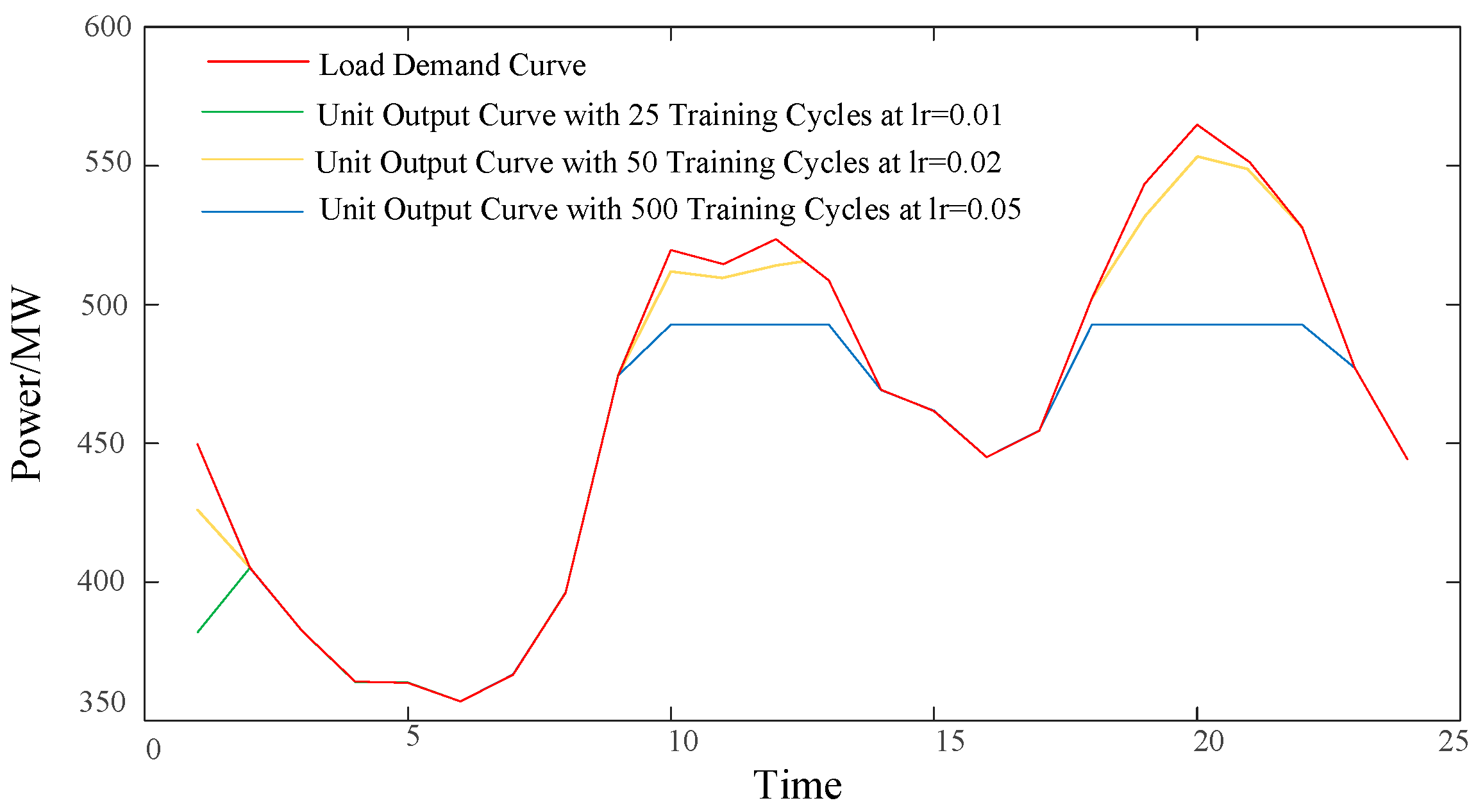
5.2. Procedural Simulation

The optimizer used for the PG network is the Adam optimizer, which uses a stochastic optimization method to give adaptive learning rates for different parameters based on the estimation of the gradient, so that it can achieve efficient computation and a low memory footprint in the optimization process. In order to choose a better learning rate parameter, lr = 0.01, lr = 0.02 and lr = 0.05 are tested, respectively. In addition, to ensure the rapid convergence and decision-making of the model, the number of training cycles of Epoch needs to be determined in the training process.

To obtain a better training effect, the convergence of the model and the fitting degree of the unit output scheme are compared in the following three cases of lr = 0.01, lr = 0.02 and lr = 0.05. The convergence process of the model with different parameters is shown in Figure 6.

It can be seen from Figure 6 that the models can converge rapidly under different parameters, which shows that the proposed UC intelligent solution algorithm based on DRL can adapt to the decision of the optimal UC scheme in a dynamic environment. When lr is 0.01, the model obtains the maximum reward value. The reason is that when the learning rate of the neural network is small, the step size in each iterative update process is shorter, so it is more accurate to guide the optimal solution. In addition, under different learning rates, when Epoch is equal to 1–10, the reward value of Epoch for each training cycle is small and fluctuates. With the increase in the number of iterations, the reward value of each iteration step increases, and finally tends to be stable when the number of training cycles of Epoch is about 30. The reason is that in the initial exploration stage of the model, the model conducts trial and error exploration according to the environment state. There is no experience to follow, and the reward value obtained is low and varied. With the continuous deepening of training, the parameters in the strategy model are constantly optimized, the strategy becomes more and more stable, and finally no longer changes. Therefore, the learning rate, lr, is set to 0.01 in this paper.

To illustrate the advantages of setting lr to 0.01, the unit decision-making scheme of 25 training cycles under lr = 0.01, the unit decision-making scheme of 50 training cycles under lr = 0.02 and the unit decision-making scheme of 200 training cycles under lr = 0.05 are given below, as shown in

Table 2. Crew decision scheme with 25 training cycles at lr = 0.01.

	G1	G2	G3	G4	G5	G6	G7	G8	G9	G10
1	0	54.406	58.293	0	0	0	85	61.819	61.353	60.895
2	0	47.971	51.398	0	79.949	97.232	74.944	0	0	53.691
3	34.061	36.331	38.927	0	60.550	73.639	56.758	41.279	0	40.662
4	32.441	34.603	37.075	0	57.669	70.135	54.057	39.315	0	38.727
5	32.420	34.581	37.051	0	57.632	70.090	54.023	39.290	0	38.702
6	31.815	33.935	36.360	0	56.557	68.782	53.014	38.556	0	37.980
7	32.666	34.843	37.333	0	58.070	70.622	54.433	39.588	0	38.996
8	35.313	37.666	40.357	0	62.775	76.344	58.843	42.796	0	42.156
9	42.288	45.106	48.329	0	75.175	91.425	70.468	51.251	0	50.484
10	46.309	49.395	52.924	0	82.323	100.11	77.170	56.124	0	55.285
11	45.857	48.914	52.408	0	81.520	99.143	76.418	55.577	0	54.746
12	46.657	49.767	53.322	0	82.943	100.87	77.751	56.547	0	55.702
13	45.324	48.345	51.798	0	80.572	97.990	75.529	54.931	0	54.109
14	41.816	44.603	47.789	0	74.336	90.405	69.682	50.679	0	49.921
15	41.139	43.881	47.016	0	73.132	88.941	68.554	49.858	0	49.113
16	39.652	42.294	45.316	0	70.488	85.726	66.075	48.055	0	47.337
17	40.503	43.202	46.289	0	72.002	87.566	67.494	49.087	0	48.353
18	44.749	47.732	51.142	0	79.551	96.748	74.571	54.235	0	53.424
19	48.422	51.649	55.339	0	86.079	104.68	80.691	58.686	0	57.808
20	50.329	53.684	57.519	0	89.471	108.81	83.871	60.998	0	60.086
21	49.129	52.404	56.148	0	87.338	106.21	81.871	59.543	0	58.653
22	47.027	50.161	53.744	0	83.599	101.67	78.366	56.995	0	56.143
23	42.513	45.347	48.586	0	75.576	91.913	70.844	51.524	0	50.754
24	39.580	42.218	45.234	0	70.361	85.570	65.955	47.968	0	47.251

,

Table 3. Crew decision scheme with 50 training cycles at lr = 0.02.

	G1	G2	G3	G4	G5	G6	G7	G8	G9	G10
1	64.835	0	45.853	0	54.227	71.032	75.693	58.345	0	47.322
2	42.692	0	50.518	0	57.841	76.693	63.357	51.071	0	43.625
3	39.085	0	34.517	0	53.654	52.954	67.542	66.882	0	57.365
4	31.196	0	46.358	0	46.743	51.771	64.286	63.614	0	42.573
5	48.391	0	42.148	0	47.714	61.981	72.514	45.564	0	45.986
6	41.1	0	45.768	0	64.641	57.438	64.641	50.511	0	42.839
7	40.787	0	45.069	0	75.902	67.915	52.215	54.754	0	52.082
8	48.221	0	50.902	0	90.719	96.389	74.406	66.875	0	52.357
9	42.81	0	53.225	0	101.508	104.799	81.017	58.484	0	63.049
10	47.474	0	53.835	0	92.223	101.207	86.755	61.527	0	61.649
11	47.364	0	49.314	0	89.872	106.609	84.292	81.093	0	57.136
12	45.25	0	51.557	0	103.204	96.833	81.943	69.071	0	53.19
13	42.815	0	51.177	0	77.725	93.537	82.636	63.424	0	65.853
14	34.839	0	53.855	0	87.608	96.152	74.673	61.549	0	55.05
15	32.753	0	53.448	0	71.425	65.296	83.925	53.673	0	65.923
16	51.27	0	47.406	0	78.962	91.947	81.646	56.649	0	55.872
17	42.027	0	53.847	0	93.99	109.708	79.341	60.361	0	58.848
18	46.027	0	60.52	0	114.113	108.032	81.157	61.128	0	69.489
19	38.94	0	44.508	0	121.932	125.142	92.183	62.03	0	55.255
20	53.739	0	45.254	0	111.1	114.682	76.534	65.985	0	58.789
21	58.953	0	45.042	0	117.249	94.742	71.256	62.847	0	67.111
22	49.431	0	46.164	0	92.059	95.437	75.931	60.239	0	62.417
23	44.862	0	45.104	0	82.05	87.89	71.197	60.111	0	61.65
24	36.142	0	45.853	0	54.227	81.032	75.693	58.345	0	47.322

and

Table 4. Crew decision scheme with 200 training cycles at lr = 0.05.

	G1	G2	G3	G4	G5	G6	G7	G8	G9	G10
1	52.714	0	0	62.016	93.710	113.96	0	63.888	63.407	0
2	47.483	0	0	55.862	84.410	102.65	0	57.547	57.114	0
3	44.799	0	0	52.705	79.639	96.855	0	54.295	53.885	0
4	42.685	0	0	50.217	75.881	92.284	0	51.732	51.342	0
5	42.631	0	0	50.154	75.784	92.167	0	51.666	51.277	0
6	41.845	0	0	49.229	74.387	90.467	0	50.713	50.331	0
7	42.983	0	0	50.568	76.411	92.929	0	52.093	51.701	0
8	46.439	0	0	54.634	82.555	100.40	0	56.282	55.858	0
9	55.614	0	0	65.428	98.866	120.23	0	67.404	66.896	0
10	57.756	0	0	67.948	102.67	124.86	0	70	69.472	0
11	57.756	0	0	67.948	102.67	124.86	0	70	69.472	0
12	57.756	0	0	67.948	102.67	124.86	0	70	69.472	0
13	57.756	0	0	67.948	102.67	124.86	0	70	69.472	0
14	54.991	0	0	64.695	97.758	118.89	0	66.648	66.146	0
15	54.123	0	0	63.674	96.216	117.01	0	65.597	65.103	0
16	52.158	0	0	61.363	92.722	112.76	0	63.215	62.739	0
17	53.283	0	0	62.686	94.722	115.19	0	64.578	64.092	0
18	57.756	0	0	67.948	102.67	124.86	0	70	69.472	0
19	57.756	0	0	67.948	102.67	124.86	0	70	69.472	0
20	57.756	0	0	67.948	102.67	124.86	0	70	69.472	0
21	57.756	0	0	67.948	102.67	124.86	0	70	69.472	0
22	57.756	0	0	67.948	102.67	124.86	0	70	69.472	0
23	55.926	0	0	65.795	99.420	120.91	0	67.782	67.271	0
24	52.063	0	0	61.251	92.554	112.56	0	63.085	62.624	0

, respectively.

In order to visually show the difference between the three cases, the sum of their output at each time is compared with the load demand curve, and the results are shown in Figure 7.

As shown in Figure 7, when lr is set to 0.01, the unit output scheme obtained after 25 cycles of iterative training can completely fit the load demand curve except that there is a certain difference between the unit output and the load demand at the first moment. When lr is set to 0.02, the unit output curve obtained after 50 cycles of iterative training has a certain power gap with the load demand at the first moment and during the two peak periods of 9–13 and 19–22, the maximum of which is 38.344 MW. When lr is set to 0.05, the unit output curve obtained after 200 cycles of iterative training has a large power gap with the load demand during the two peak periods of 9–14 and 19–23, with a maximum of 72.06 MW. The reason for this is that when lr is set to 0.02 and 0.05, after 50 and 200 training iterations, the unit output scheme meeting the current load demand is still not solved. While when lr is set to 0.01, the unit output scheme meeting the constraint conditions can be quickly solved after 25 iterative training cycles.

After a large number of simulation tests, it is found that when the relevant hyperparameters in the DRL algorithm are set according to the data shown in

Table 5. DRL algorithm super parameter.

Learning Rate	0.01
Reward Decay Rate	0.95
Memory size	500
Batch size	24
Epochs	30
Optimization Solution Method	Adam

, the model can converge quickly and the effect is good.

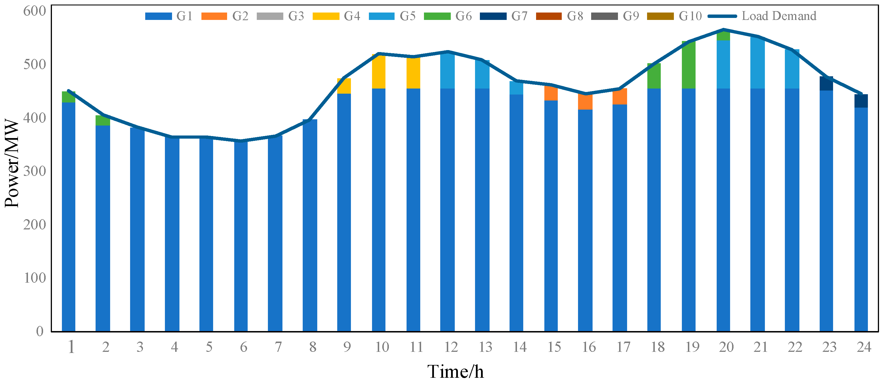
5.3. Comparative Analysis

In this paper, the advantages of this method over the traditional method are illustrated by comparing the unit output scheme, decision-making time and cost or reward value of Method 1, Method 2 and Method 3.

Method 1: Based on the physical model-driven UC decision-making method.

Method 2: The data-driven UC decision-making method of reference [7].

Method 3: An intelligent decision-making method for UC based on DRL, namely the method in this paper.

The unit output schemes obtained using the three methods are shown in Figure 8, Figure 9 and Figure 10, respectively.

It can be seen from Figure 8, Figure 9 and Figure 10 that in Method 1, under the current load demand, most of the output is borne by Unit 1, accounting for about 85% of the load demand, and the rest is borne by the combination of Unit 2, Unit 4, Unit 5, Unit 6 and Unit 7. Similarly, in Method 2, under the current load demand, most of the output is borne by Unit 1, but most of the output converts into Unit 2 during the 15–19 peak periods, and the rest is borne by the combination of Unit 3, Unit 5, Unit 6, Unit 9 and Unit 10. In contrast, in Method 3, most of the load is not borne by one unit, but by all the unit combinations except Unit 5, Unit 7, and the Unit 10. In order to analyze the reasons, the decision time and the system operation cost or reward value of the three methods are given below.

The difference between the unit output schemes of three methods is also reflected in

Table 6. Decision time and system operation cost/reward value of three methods.

Method	Training Time/s	Decision Time/s	Cost Or Reward Value/CNY
Method 1	-	3938.16	228,200
Method 2	97.54	0.31	236,910
Method 3	2.13	0.43	304,339

, in which the reward value obtained via Method 3 is more than CNY 76,000 higher than the system cost of Method 1 and more than CNY 67,000 higher than the system cost of Method 2. The reasons are as follows. On the one hand, compared with the decision result of Method 1 and Method 2, the decision result of Method 3 obviously does not reach the global optimum, so the system operation cost contained in the reward value is higher than that of Method 1 and Method 2. On the other hand, the reward value in Method 3 consists of the system operation cost and the penalty obtained by violating the constraints. Because the unit output scheme at a certain time in the decision result of this method does not meet the load balance constraint, it also includes part of the penalty amount. For the above reasons, the reward value obtained via Method 3 is higher than the system operating cost of other methods.

In terms of decision-making efficiency, the decision-making time of Method 1 is 3938.16 s. Method 2 requires a large amount of historical data to train the model, so the training time takes 97.54 s, but the decision time only takes 0.31 s. In Method 3, although the model needs to interact with the environment in the training stage, constantly explore trial and error, and gradually find the action strategy with the maximum reward value in the limited action space, it only takes 2.13 s. After the training, it takes only 0.43 s to obtain the UC decision scheme according to this strategy. The total time of Method 3 decreases by 3935.6 s and 95.29 s compared to Methods 1 and 2. To sum up, although the UC intelligent solution algorithm based on DRL does not reach the final optimal combination state, it improves solution efficiency to a certain extent compared to that of the UC decision method based on the physical model driven in terms of training time and decision time.

In order to obtain a better combination state under Method 3, the iteration times are increased to 300 and 500 to see the change of the decision results. The output schemes of the units in the two cases are shown in Figure 11 and Figure 12.

It can be seen from Figure 11 and Figure 12 that when the number of iterations is 300, there is a power shortage during part of the peak hours from 9 to 24. When the number of iterations is set to 500, the system unit output can meet the load demand at any time in the scheduling period, and there is no power shortage. Therefore, the DRL-based intelligent UC algorithm proposed in this paper is correct and effective in the decision-making of small-scale UC problems.

6. Conclusions

In this paper, DRL is applied to the field of UC, and an intelligent algorithm for solving UC based on DRL is proposed. In order to facilitate the solution, the UC problem is divided into two steps for calculation. The first one is to decide the start and stop state of the unit in each period. The second one is to solve the corresponding output of the unit according to the start and stop state. In the first step, the DRL algorithm is used to construct the MDP model of UC problem. Based on the characteristics of the UC problem, the state space, action space, transition function and reward function are given. The PG algorithm is used to solve the problem, and the model makes decisions according to the strategy mapped from the state to the action. In the second step, Lambda iteration is used to solve the output of the unit according to the current startup and shutdown status of the unit. The following conclusions can be drawn from the simulation example:

(1)

The intelligent solving algorithm of UC based on DRL proposed in this paper can effectively decide complex small-scale UC problems, and has high applicability.

(2)

Compared to supervised learning, the method does not require the construction of a large number of labeled sample data in advance, avoids the dependence on sample data, and has higher generalization performance.

(3)

Compared to the traditional method, this method can directly give the action decision through the strategy model of the model, and the solving efficiency is higher.

References

1. Zhao, H.; Wang, Y.; Guo, S.; Zhao, M.; Zhang, C. Application of a Gradient Descent Continuous Actor-Critic Algorithm for Double-Side Day-Ahead Electricity Market Modeling. Energies 2016, 9, 725. [Google Scholar] [CrossRef] [Green Version]
2. Wang, C.; Chu, S.; Ying, Y.; Wang, A.; Chen, R.; Xu, H.; Zhu, B. Underfrequency Load Shedding Scheme for Islanded Microgrids Considering Objective and Subjective Weight of Loads. IEEE Trans. Smart Grid 2023, 14, 899–913. [Google Scholar] [CrossRef]
3. Zhu, B.; Liu, Y.; Zhi, S.; Wang, K.; Liu, J. A Family of Bipolar High Step-Up Zeta–Buck–Boost Converter Based on “Coat Circuit. IEEE Trans. Power Electron. 2023, 38, 3328–3339. [Google Scholar] [CrossRef]
4. Bertsimas, D.; Litvinov, E.; Sun, X.; Zhao, J.; Zheng, T. Adaptive Robust Optimization for the Security Constrained Unit Commitment Problem. IEEE Trans. Power Syst. A Publ. Power Eng. Soc. 2013, 28, 52–63. [Google Scholar] [CrossRef]
5. Li, Z.; Jiang, W.; Abu-Siada, A.; Li, Z.; Xu, Y.; Liu, S. Research on a Composite Voltage and Current Measurement Device for HVDC Networks. IEEE Trans. Ind. Electron. 2021, 68, 8930–8941. [Google Scholar] [CrossRef]
6. Chen, J.J.; Qi, B.X.; Rong, Z.K.; Peng, K.; Zhao, Y.L.; Zhang, X.H. Multi-energy coordinated microgrid scheduling with integrated demand response for flexibility improvement. Energy 2021, 217, 119387. [Google Scholar] [CrossRef]
7. Liao, S.; Xu, J.; Sun, Y.; Bao, Y.; Tang, B. Control of Energy-intensive Load for Power Smoothing in Wind Power Plants. IEEE Trans. Power Syst. 2018, 33, 6142–6154. [Google Scholar] [CrossRef]
8. Zhou, Y.; Zhai, Q.; Wu, L. Optimal operation of regional microgrids with renewable and energy storage: Solution robustness and nonanticipativity against uncertainties. IEEE Trans. Smart Grid 2022, 13, 4218–4230. [Google Scholar] [CrossRef]
9. Yu, G.; Liu, C.; Tang, B.; Chen, R.; Lu, L.; Cui, C.; Hu, Y.; Shen, L.; Muyeen, S.M. Short term wind power prediction for regional wind farms based on spatial-temporal characteristic distribution. Renew. Energy 2022, 199, 599–612. [Google Scholar] [CrossRef]
10. Yang, N.; Jia, J.; Xing, C.; Liu, S.; Chen, D.; Ye, D.; Deng, Y. Data-driven intelligent decision-making method for unit commitment based on E-Seq2Seq technology. Proc. CSEE 2020, 40, 7587–7600. [Google Scholar]
11. Shi, L.; Zhai, F. Data-driven unit commitment model considering wind-light-load uncertainty. Integr. Smart Energy 2022, 44, 18–25. [Google Scholar]
12. Zhang, Y.; Ai, X.; Fang, J.; Wu, M.; Yao, W.; Wen, J. Data-driven robust unit commitment based on generalized convex hull uncertainty set. Proc. CSEE 2020, 40, 477–487. [Google Scholar]
13. Yang, N.; Ye, D.; Lin, J.; Huang, Y.; Dong, B.; Hu, W.; Liu, S. Research on intelligent decision-making method of unit commitment based on data-driven and self-learning ability. Proc. CSEE 2019, 39, 2934–2946. [Google Scholar]
14. Zhang, L.; Luo, Y. Combined Heat and Power Scheduling: Utilizing Building-level Thermal Inertia for Short-term Thermal Energy Storage in District Heat System. IEEJ Trans. Electr. Electron. Eng. 2018, 13, 804–814. [Google Scholar] [CrossRef]
15. Jaderberg, M.; Czarnecki, W.M.; Dunning, I.; Marris, L.; Lever, G.; Castañeda, A.G.; Beattie, C.; Rabinowitz, N.C.; Morcos, A.S.; Ruderman, A.; et al. Human-level performance in 3D multiplayer games with population-based reinforcement learning. Science 2019, 364, 859–865. [Google Scholar] [CrossRef] [Green Version]
16. Marot, A.; Donnot, B.; Romero, C.; Donon, B.; Lerousseau, M.; Veyrin-Forrer, L.; Guyon, I. Learning to run a power network challenge for training topology controllers. Electr. Power Syst. Res. 2020, 189, 106635. [Google Scholar] [CrossRef]
17. Ahamed, T.P.; Imthias, P.S.; Nagendra Rao, P.; Sastry, S. A reinforcement learning approach to automatic generation control. Electr. Power Syst. Res. 2002, 63, 9–26. [Google Scholar] [CrossRef] [Green Version]
18. Mevludin, G.; Ernst, D.; Wehenkel, L. A reinforcement learning based discrete supplementary control for power system transient stability enhancement. Int. J. Eng. Intell. Syst. Electr. Eng. Commun. 2005, 13, 81–88. [Google Scholar]
19. Gajjar, G.R.; Khaparde, S.A.; Nagaraju, P. Application of actor-critic learning algorithm for optimal bidding problem of a Genco. IEEE Trans. Power Syst. A Publ. Power Eng. Soc. 2003, 18, 11–18. [Google Scholar] [CrossRef]
20. Fang, P.; Fu, W.; Wang, K.; Xiong, D.; Zhang, K. A compositive architecture coupling outlier correction, EWT, nonlinear Volterra multi-model fusion with multi-objective optimization for short-term wind speed forecasting. Appl. Energy 2022, 307, 118191. [Google Scholar] [CrossRef]
21. Nan, Y.; Cong, Y.; Chao, X.; Di, Y.; Junjie, J.; Daojun, C.; Xun, S.; Yuehua, H.; Lei, Z.; Binxin, Z. Deep learning-based SCUC decision-making: An intelligent data-driven approach with self-learning capabilities. IET Gener. Transm. Distrib. 2022, 16, 629–640. [Google Scholar]
22. Yang, N.; Dong, Z.; Wu, L.; Zhang, L.; Shen, X.; Chen, D.; Zhu, B.; Liu, Y. A Comprehensive Review of Security-constrained Unit Commitment. J. Mod. Power Syst. Clean Energy 2022, 10, 562–576. [Google Scholar] [CrossRef]
23. Zhang, Y.; Xie, X.; Fu, W.; Chen, X.; Hu, S.; Zhang, L.; Xia, Y. An Optimal Combining Attack Strategy Against Economic Dispatch of Integrated Energy System. IEEE Trans. Circuits Syst. II Express Briefs 2023, 70, 246–250. [Google Scholar] [CrossRef]
24. Yang, N.; Yang, C.; Wu, L.; Shen, X.; Jia, J.; Li, Z.; Chen, D.; Zhu, B.; Liu, S. Intelligent Data-Driven Decision-Making Method for Dynamic Multisequence: An E-Seq2Seq-Based SCUC Expert System. IEEE Trans. Ind. Inform. 2022, 18, 3126–3137. [Google Scholar] [CrossRef]
25. Ma, H.; Zheng, K.; Jiang, H.; Yin, H. A family of dual-boost bridgeless five-level rectifiers with common-core inductors. IEEE Trans. Power Electron. 2021, 36, 12565–12578. [Google Scholar] [CrossRef]
26. Fu, W.; Jiang, X.; Li, B.; Tan, C.; Chen, B.; Chen, X. Rolling Bearing Fault Diagnosis based on 2D Time-Frequency Images and Data Augmentation Technique. Meas. Sci. Technol. 2023, 34, 045005. [Google Scholar] [CrossRef]
27. Zhang, Y.; Wei, L.; Fu, W.; Chen, X.; Hu, S. Secondary frequency control strategy considering DoS attacks for MTDC system. Electr. Power Syst. Res. 2023, 214, 108888. [Google Scholar] [CrossRef]
28. Yang, N.; Qin, T.; Wu, L.; Huang, Y.; Huang, Y.; Xing, C.; Zhang, L.; Zhu, B. A multi-agent game based joint planning approach for electricity-gas integrated energy systems considering wind power uncertainty. Electr. Power Syst. Res. 2021, 204, 107673. [Google Scholar] [CrossRef]
29. Xie, K.; Hui, H.; Ding, Y. Review of modeling and control strategy of thermostatically controlled loads for virtual energy storage system. Prot. Control Mod. Power Syst. 2019, 4, 23. [Google Scholar] [CrossRef]
30. Badal, F.R.; Das, P.; Sarker, S.K.; Das, S.K. A survey on control issues in renewable energy integration and microgrid. Prot. Control Mod. Power Syst. 2019, 4, 8. [Google Scholar] [CrossRef] [Green Version]
31. Shen, X.; Raksincharoensak, P. Pedestrian-Aware Statistical Risk Assessment. IEEE Trans. Intell. Transp. Syst. 2022, 23, 7910–7918. [Google Scholar] [CrossRef]
32. Li, Z.; Yub, C.; Abu-Siadac, A.; Lid, H.; Lia, Z.; Zhangb, T.; Xub, Y. An online correction system for electronic voltage transformers. Int. J. Electr. Power Energy Syst. 2021, 126, 106611. [Google Scholar] [CrossRef]
33. Zhengmao, L.; Lei, W.; Yan, X. Risk-Averse Coordinated Operation of a Multi-Energy Microgrid Considering Voltage/Var Control and Thermal Flow: An Adaptive Stochastic Approach. IEEE Trans. Smart Grid 2021, 12, 3914–3927. [Google Scholar]
34. Yang, N.; Liang, J.; Ding, L.; Zhao, J.; Xin, P.; Jiang, J.; Li, Z. Integrated Optical Storage Charging Considering Reconstruction Expansion and Safety Efficiency Cost. Grid Technol. 2023, 1–13. [Google Scholar] [CrossRef]
35. Xu, P.; Fu, W.; Lu, Q.; Zhang, S.; Wang, R.; Meng, J. Stability analysis of hydro-turbine governing system with sloping ceiling tailrace tunnel and upstream surge tank considering nonlinear hydro-turbine characteristics. Renew. Energy 2023, 210, 556–574. [Google Scholar] [CrossRef]
Figure 1. DRL-based UC intelligent solution algorithm decision block diagram.
Sustainability 15 11084 g001
Figure 2. Solution process.
Sustainability 15 11084 g002
Figure 3. Lambda iteration flow chart.
Sustainability 15 11084 g003
Figure 4. Graphic method for solving economic dispatch problems.
Sustainability 15 11084 g004
Figure 5. Estimation of Lambda value via interpolation method.
Sustainability 15 11084 g005
Figure 6. Model convergence during training.
Sustainability 15 11084 g006
Figure 7. Comparison of unit output curve and load demand curve under three conditions.
Sustainability 15 11084 g007
Figure 8. Unit output scheme of Method 1.
Sustainability 15 11084 g008
Figure 9. Unit output scheme of Method 2.
Sustainability 15 11084 g009
Figure 10. Unit output scheme of Method 3.
Sustainability 15 11084 g010
Figure 11. Unit output scheme for 300 iterations.
Sustainability 15 11084 g011
Figure 12. Unit output scheme for 500 iterations.
Sustainability 15 11084 g012