Interpretable Machine Learning for Assessing the Cumulative Damage of a Reinforced Concrete Frame Induced by Seismic Sequences

Abstract

Recently developed Machine Learning (ML) interpretability techniques have the potential to explain how predictors influence the dependent variable in high-dimensional and non-linear problems. This study investigates the application of the above methods to damage prediction during a sequence of earthquakes, emphasizing the use of techniques such as SHapley Additive exPlanations (SHAP), Partial Dependence Plots (PDPs), Local Interpretable Model-agnostic Explanations (LIME), Accumulated Local Effects (ALE), permutation and impurity-based techniques. Following previous investigations that examine the interdependence between predictors and the cumulative damage caused by a seismic sequence using classic statistical methods, the present study deploy ML interpretation techniques to deal with this multi-parametric and complex problem. The research explores the cumulative damage during seismic sequences, aiming to identify critical predictors and assess their influence on the cumulative damage. Moreover, the predictors contribution with respect to the range of final damage is evaluated. Non-linear time history analyses are applied to extract the seismic response of an eight-story Reinforced Concrete (RC) frame. The regression problem’s input variables are divided into two distinct physical classes: pre-existing damage from the initial seismic event and seismic parameters representing the intensity of the subsequent earthquake, expressed by the Park and Ang damage index ($\mathrm{D}{\mathrm{I}}_{\mathrm{P}\mathrm{A}}$) and Intensity Measures (IMs), respectively. In addition to the interpretability analysis, the study offers also a comprehensive review of ML methods, hyperparameter tuning, and ML method comparisons. A LightGBM model emerges as the most efficient, among 15 different ML methods examined. Among the 17 examined predictors, the initial damage, caused by the first shock, and the IMs of the subsequent shock—${\mathrm{I}}_{\mathrm{F}\mathrm{V}\mathrm{F}}$ and $\mathrm{S}{\mathrm{I}}_{\mathrm{H}}$—emerged as the most important ones. The novel results of this study provide useful insights in seismic design and assessment taking into account the structural performance under multiple moderate to strong earthquake events.

1. Introduction

Earthquake series that occurs in succession causes additional damage on already damaged buildings and therefore increases the risk of a collapse. Historical examples of seismic sequences include the New Madrid (1811–1812) sequence [1], which comprised three primary shocks and several aftershocks. The events caused extensive structural damage, affecting regions as far as Canada on the north side and eastern United States. The 1960 Chilean sequence [2] initiated by the historic 9.5 magnitude mainshock led to massive devastation and life losses in Chile and triggered a series of tsunamis. One notable seismic sequence occurred in central Italy in 2016 where over a period of several months, there was a succession of earthquakes with a 6.2 magnitude mainshock leading to significant destruction and casualties [3,4]. Experts studying the series of seismic events found that they transpired on pre-existing fault lines that had been under stress for a considerable period of time. Moreover, they ascertained that the earthquake sequence had shifted the stress distribution within the region, hence potentially increasing the probability of subsequent seismic events. Another example is the 2019 Ridgecrest sequence [5] in California, which included a mainshock of 6.4, then several aftershocks including of a 7.1 seismic event. This sequence resulted in extensive damage to infrastructure and homes in the region. Accordingly, it demonstrated the potential for aftershocks to be almost as powerful as the mainshock. In February 2023, southeastern Türkiye and parts of Syria were hit by two strong earthquakes resulting in numerous aftershocks and significant loss of life and injuries [6,7]. The earthquakes had magnitudes of 7.8 and 7.5 and occurred approximately nine hours apart. As an outcome of all the above examples, the assessment of cumulative damage and vulnerability of structures or buildings to multiple earthquakes needs to be determined to avert or minimize potential losses.

Several studies focus on the effect of multiple earthquake events on the seismic performance of Reinforced Concrete (RC) structures. Abdelnaby in his PhD thesis [8] examines the consequences that successive seismic events have on RC buildings’ degradation. Later, Hatzivassiliou and Hatzigeorgiou [9] investigate the effect of seismic sequences on the response of three-dimensional RC buildings, while Kavvadias et al. [10] examine the impact of aftershock severity characteristics on the seismic damage of a RC frame. Trevlopoulos and Guéguen [11] propose a framework to assess the vulnerability of RC structures during aftershock sequences based on period elongation. Additional research in this field encompasses the work of Shokrabadi et al. [12], who explore the influence of coupling mainshock-aftershock (MS-AS) ground motions on seismic behaviour. Furthermore, Furtado et al. [13] evaluate the structural damage of reinforced concrete (RC) buildings with infill walls subjected to MS-AS scenarios. Di Sarno and Pugliese [14] study the seismic fragility of existing RC buildings with corroded bars under earthquake sequences, while Iervolino et al. [15] examine the accumulation of seismic damage in multiple MS-AS sequences. Rajabi and Ghodrati Amiri [16] develop behaviour factor prediction equations for RC frames under critical MS-AS sequences using Artificial Neural Networks (ANNs). Soureshjani and Massumi [17] investigate the seismic behaviour of RC moment-resisting structures with concrete shear walls under MS-AS seismic sequences. Khansefid [18] studies the effect of structural non-linearity on the risk estimation of buildings under MS-AS sequences in Tehran metro city. Additionally, Hu et al. [19] introduce a framework for the seismic resilience assessment of buildings that considers the effects of both mainshock and multiple aftershocks. Finally, Askouni [20] investigate how repeated earthquakes affect RC buildings with in-plan irregularities. Overall, the research findings demonstrate the importance of considering the effects of multiple earthquakes in the design and assessment of RC structures.

The capability of Machine Learning (ML) to predict the behaviour of structures has spurred interest in earthquake and structural engineering. The early papers [21,22] in this field are applications of ANNs either for purposes of response prediction of simple structures or non-destructive elastostatic identification of unilateral cracks. Later studies [23,24], dealt with non-linear seismic responses of 2D and 3D buildings using ANN and proved that this ML method can be used to accurately predict the behaviour of complex structures. In addition, Hybrid ML techniques have been investigated for the prediction of structural damage under earthquake excitation [25,26,27], while Mangalathu et al. [28], as well as Wang et al. [29], used ML techniques for classifying buildings on post-earthquake observations. Recent papers [30,31,32] also have explored the use of deep learning, which has shown great promise in rapid seismic response prediction of RC frames. Physics-guided neural networks have been used for data-driven seismic response modelling [33], elastic plate problems [34], and static rod and beam problems [35]. In that respect, more recent papers investigate the application of ML in seismic response prediction. For example, Morfidis and Kostinakis [36] predicted the damage state of RC buildings using ANNs while Hwang et al. [37] predicted both seismic demand, as well as collapse for ductile RC building frames using ML methods. In some other cases too, earthquake scenarios for building portfolios have been developed [38], rapid seismic response prediction has also been conducted [39], plus multivariate seismic classification [40]. Kazemi et al. [41] presented a ML-based approach for the classification of the structural behaviour of tall buildings with a diagrid structure. Karbassi et al. [42] and Ghiasi et al. [43] proposed decision tree and support vector machine algorithms, respectively, to predict damage in RC buildings, while Chen et al. [44], and Jia and Wu [45] investigated probabilistic ML methods for predicting the performance of structures and infrastructures. Furthermore, the literature has showcased numerous instances of using ML to evaluate the seismic fragility and risk of civil engineering structures [46,47,48,49,50,51]. Moreover, Morfidis et al. [52] developed a user-friendly software application that leverages ANNs for rapid damage assessment of RC buildings in earthquake scenarios. Lastly, Lazaridis et al. [53,54] presented studies on forecasting the structural damage experienced by a RC frame subjected to both individual and successive seismic events using ML methods. Additional information regarding the application of ML in the field of earthquake and structural engineering can be found in the respective review papers [55,56,57,58,59,60,61,62,63,64].

The majority of the above ML applications in earthquake engineering consider only the damages from individual earthquakes, ignoring that in most cases the seismic events occurred in succession and cause cumulative damage to buildings. To the best of authors’ knowledge, the influence of potential predictors on cumulative structural damage under sequential earthquakes, using ML interpretation methods, has not been presented in the literature yet. In related past studies, the effect of predictors on the cumulative structural damage has been evaluated by employed Pearson or Spearman correlation coefficients [10,65,66] and consequently did not efficiently model this multi-parametric and complex non-linear problem. Moreover, ML techniques have been used for the explanation of seismic damage prediction in other studies [67], considering structural damage caused only by individual earthquakes. Additionally, the problem of cumulative seismic damage prediction has been examined by the authors of [54] without providing insights or interpretation of the ML models. Moreover, the cumulative damage to buildings from successive earthquakes has not been considered in seismic codes, until now.

In this study, the extension of interpretation techniques to include the concept of cumulative damage during a sequence of earthquakes has been undertaken. The primary objective of this study is to discover the key parameters which ought to have high priority by the earthquake and structural engineering community while designing against seismic events involving a sequence of earthquakes. In addition, it will also show how ML can help in handling the high non-linear problem of structural response under sequential earthquake excitations. For this scope, 15 ML methods which are appropriate for tabular data, as the data examined in this study, were selected from the literature. Using the randomized search cross-validation process, different variants with different hyperparameter values for every method were picked. Each variant was trained and evaluated using the K-fold cross-validation strategy on the training set to indicate the best model and complete the hyperparameter tuning. The global interpretation techniques are applied to the best model for identification of general predictors behaviours, while local and global explanation methods are used for extracting feature importances. In summary, the primary questions addressed in the present paper include: identifying the most important predictors for damage accumulation, understanding how these variables impact the final damage, and determining the range of cumulative damage in which their contributions lie.

2. Feature Selection and Dataset Configuration and Preprocessing

The input variables for our regression problem fall into two distinct physical classes: the pre-existing damage from the initial seismic event, along with the seismic parameters representing the intensity of the subsequent earthquake. The objective is to predict the cumulative damage occurred by two consecutive earthquakes. The first class of feature, as well as the target, is expressed in terms of the Park and Ang damage index ($\mathrm{D}{\mathrm{I}}_{\mathrm{P}\mathrm{A}}$) [68]. For the second category, a preliminary feature selection process has been conducted. During this process, the outcomes of several studies [36,69,70,71,72,73,74,75,76,77] investigating the interdependence between seismic parameters and damage indicators of RC structures have been taken into account. As a result, 16 prominent Intensity Measures (IMs) have been selected as seismic damage predictors to express the severity of the second shock. The selected IMs, as well as the damage index, are described in the following section.

2.1. Ground Motion IMs and Damage Index

2.1.1. Ground Motion IMs

Seismic ground motion IMs are metrics employed to quantify the intensity or severity of seismic acceleration signals. These measures play a crucial role in evaluating a site’s seismic hazard, predicting seismic demand on structures, and designing earthquake-resistant structures. Various IMs have been suggested over time, each with its own pros and cons. Peak Ground Acceleration (PGA) [78] is among the most commonly used ground motion signal IMs. PGA represents the maximum absolute acceleration of ground motion during an earthquake and is extensively used in seismic hazard analysis and building design, as it offers a straightforward indication of ground shaking intensity. Furthermore, our suite of IMs encompass amplitude parameters such as the maximum absolute values of ground velocity (PGV), and ground displacement (PGD) signals. The Arias intensity (${\mathrm{I}}_{\mathrm{A}}$) [79] and Cumulative Absolute Velocity (CAV) [78] are additional seismic ground motion IMs that supply information about the overall amount of ground motion energy during an earthquake. Both ${\mathrm{I}}_{\mathrm{A}}$ and $\mathrm{C}\mathrm{A}\mathrm{V}$ are determined as integrals of ground motion acceleration over time, offering a more comprehensive depiction of the seismic signal compared to PGA or PGV, as they account for both the amplitude and duration of the signal.

The frequency content of ground motion signals significantly influences a structure’s response. This content can be assessed in a simplified manner using the corresponding frequency PGA/PGV or by calculating the average zero-crossing count of the acceleration time history per unit time. If the number of zero-crossings is denoted as ${\mathrm{u}}_{\mathrm{o}}$, the fraction of ${\mathrm{I}}_{\mathrm{A}}$ over ${\mathrm{u}}_{\mathrm{o}}^2$ is recognized as the potential destructiveness measure, according to Araya and Saragoni (${\mathrm{I}}_{\mathrm{A}\mathrm{S}}$) [80]. The strong motion duration of seismic excitation considering as the time interval during which most of the total intensity is released, is another vital parameter. Two definitions of strong motion duration, Trifunac and Brady ($\mathrm{S}\mathrm{M}{\mathrm{D}}_{\mathrm{T}\mathrm{B}}$) [81] and Reinoso, Ordaz, and Guerrero ($\mathrm{S}\mathrm{M}{\mathrm{D}}_{\mathrm{R}\mathrm{O}\mathrm{G}}$) [82], are based on the Arias intensity’s time evolution. The bracketed duration after Bolt ($\mathrm{S}\mathrm{M}{\mathrm{D}}_{\mathrm{B}\mathrm{o}\mathrm{l}\mathrm{t}}$) [83], which is calculated based on the initial and final instances when the acceleration exceeds 5% of g, is also utilized.

Advanced measures can be obtained by merging the above parameters, such as power P90 [78], ${\mathrm{a}}_{\mathrm{r}\mathrm{m}\mathrm{s}}$[78], characteristic intensity (${\mathrm{I}}_{\mathrm{c}}$) [78], the potential damage metric by Fajfar, Vidic, and Fischinger (${\mathrm{I}}_{\mathrm{F}\mathrm{V}\mathrm{F}}$) [84], and the intensity measure by Riddell and Garcia (${\mathrm{I}}_{\mathrm{R}\mathrm{G}}$) [85]. However, spectral values reliant on the fundamental structural period are not applicable due to the increase in the fundamental period during the initial earthquake. As an alternative, the Housner intensity ($\mathrm{S}{\mathrm{I}}_{\mathrm{H}}$) [86], which aggregates the values of pseudo-velocity spectrum ($\mathrm{P}\mathrm{S}\mathrm{V}$) to a constant interval of periods and exhibits a strong correlation with seismic damage, is utilized. A brief depiction of the formulas for the studied IMs is given in

Table 1. Mathematical formulas of the examined IMs [54].

Num	Name	Expression	Ref.	Num	Name	Expression	Ref.
1	$\mathrm{P}\mathrm{G}\mathrm{A}$	$\mathrm{m}\mathrm{a}\mathrm{x}|{\mathrm{a}}_{\mathrm{g}}\left(\mathrm{t}\right)|$	[78]	9	$\mathrm{S}\mathrm{M}{\mathrm{D}}_{\mathrm{R}\mathrm{O}\mathrm{G}}$	$\mathrm{t}({\mathrm{H}}_{\mathrm{d}}=97.5\%)-\mathrm{t}({\mathrm{H}}_{\mathrm{d}}=2.5\%)$  *	[82]
2	$\mathrm{P}\mathrm{G}\mathrm{V}$	$\mathrm{m}\mathrm{a}\mathrm{x}|{\mathrm{v}}_{\mathrm{g}}\left(\mathrm{t}\right)|$	[78]	10	$\mathrm{S}\mathrm{M}{\mathrm{D}}_{\mathrm{B}\mathrm{o}\mathrm{l}\mathrm{t}}$	${\mathrm{t}}_{\mathrm{l}\mathrm{a}\mathrm{s}\mathrm{t}}^{{\mathrm{a}}_{\mathrm{g}}>0.05\mathrm{g}}-{\mathrm{t}}_{1\mathrm{s}\mathrm{t}}^{{\mathrm{a}}_{\mathrm{g}}>0.05\mathrm{g}}$	[83]
3	$\mathrm{P}\mathrm{G}\mathrm{D}$	$\mathrm{m}\mathrm{a}\mathrm{x}|{\mathrm{d}}_{\mathrm{g}}\left(\mathrm{t}\right)|$	[78]	11	${\mathrm{P}}_{90}$	$\frac{{\mathrm{I}}_{\mathrm{A}}({\mathrm{H}}_{\mathrm{d}}=95\%)-{\mathrm{I}}_{\mathrm{A}}({\mathrm{H}}_{\mathrm{d}}=5\%)}{\mathrm{S}\mathrm{M}{\mathrm{D}}_{\mathrm{T}\mathrm{B}}}$	[78]
4	${\mathrm{I}}_{\mathrm{A}}$	$\frac{\pi }{2\mathrm{g}}{\int }_0^{{\mathrm{t}}_{\mathrm{e}\mathrm{n}\mathrm{d}}}{\mathrm{a}}_{\mathrm{g}}^2\left(\mathrm{t}\right)\mathrm{d}\mathrm{t}$	[79]	12	${\mathrm{a}}_{\mathrm{r}\mathrm{m}\mathrm{s}}$	$\sqrt{\frac{1}{\mathrm{S}\mathrm{M}{\mathrm{D}}_{\mathrm{T}\mathrm{B}}}{\int }_{{\mathrm{t}}_{5\%}}^{{\mathrm{t}}_{95\%}}{\mathrm{a}}_{\mathrm{g}}{\left(\mathrm{t}\right)}^2\mathrm{d}\mathrm{t}}$	[78]
5	$\mathrm{C}\mathrm{A}\mathrm{V}$	${\int }_{\mathrm{o}}^{{\mathrm{t}}_{\mathrm{e}\mathrm{n}\mathrm{d}}}\left|{\mathrm{a}}_{\mathrm{g}}\left(\mathrm{t}\right)\right|\mathrm{d}\mathrm{t}$	[78]	13	${\mathrm{I}}_{\mathrm{c}}$	${\mathrm{a}}_{\mathrm{r}\mathrm{m}\mathrm{s}}^{1.5}·\mathrm{S}\mathrm{M}{\mathrm{D}}_{\mathrm{T}\mathrm{B}}^{0.5}$	[78]
6	$\mathrm{P}\mathrm{G}\mathrm{A}/\mathrm{P}\mathrm{G}\mathrm{V}$	$\frac{\mathrm{P}\mathrm{G}\mathrm{A}}{\mathrm{P}\mathrm{G}\mathrm{V}}$	[78]	14	${\mathrm{I}}_{\mathrm{F}\mathrm{V}\mathrm{F}}$	$\mathrm{P}\mathrm{G}\mathrm{V}·\mathrm{S}\mathrm{M}{\mathrm{D}}_{\mathrm{T}\mathrm{B}}^{0.25}$	[84]
7	${\mathrm{I}}_{\mathrm{A}\mathrm{S}}$	$\frac{{\mathrm{I}}_{\mathrm{A}}}{{\mathrm{u}}_{\mathrm{o}}^2}$	[80]	15	${\mathrm{I}}_{\mathrm{R}\mathrm{G}}$	$\mathrm{P}\mathrm{G}\mathrm{D}·\mathrm{S}\mathrm{M}{\mathrm{D}}_{\mathrm{T}\mathrm{B}}^{\frac{1}{3}}$	[85]
8	$\mathrm{S}\mathrm{M}{\mathrm{D}}_{\mathrm{T}\mathrm{B}}$	$\mathrm{t}({\mathrm{H}}_{\mathrm{d}}=95\%)-\mathrm{t}({\mathrm{H}}_{\mathrm{d}}=5\%)$ *	[81]	16	$\mathrm{S}{\mathrm{I}}_{\mathrm{H}}$	${\int }_{0.1}^{2.5}\mathrm{P}\mathrm{S}\mathrm{V}(\mathrm{T},\xi =0.05)\mathrm{d}\mathrm{T}$	[86]

* ${\mathrm{H}}_{\mathrm{d}}$: Husid diagram [87].

.

2.1.2. Damage Index

Seismic damage in structures manifests as a reduction in resistance to external forces, resulting in instability. The Park and Ang damage index ($\mathrm{D}{\mathrm{I}}_{\mathrm{P}\mathrm{A}}$) is a reliable seismic damage metric that represents structural damage as a linear combination of excessive deformation and damage developed by repeated cyclic loading effects. This index is calculated by summing the maximum bending responses and the energy absorbed by plastic hinges during an earthquake, as shown in Equation (1). Due to this fact, the Park and Ang damage index can effectively represent the evolution of cumulative flexural damage, both for individual shocks and during a sequence of seismic events (Figure 1), in contrast with other damage indicators which capture only maximum responses and cannot represent the accumulation of damage investigated in this study. Kunnath’s modified version of the index [88] is calculated using Equation (2). The total damage index ($\mathrm{D}{\mathrm{I}}_{\mathrm{G},\mathrm{P}\mathrm{A}}$) is obtained as an adjusted mean of sub-damage values, where each sub-damage belongs to each structural member. The weight of each sub-damage is proportional to the energy used by its corresponding structural member, according to Equation (3). A low value of $\mathrm{D}{\mathrm{I}}_{\mathrm{G},\mathrm{P}\mathrm{A}}$, close to zero, indicates that the structure has experienced minimal damage and exhibited an elastic response. Conversely, a value around the unity and larger signifies that the structure is near collapse. Overall damage indices, such as $\mathrm{D}{\mathrm{I}}_{\mathrm{G},\mathrm{P}\mathrm{A}}$, offer a quantitative assessment of a structure’s seismic damage and have been utilized in several studies [36,69,70,71,72,76,89] to evaluate the post-earthquake condition of buildings.

$$\mathrm{D}{\mathrm{I}}_{\mathrm{P}\mathrm{A}}=\frac{{\delta }_{\mathrm{m}}}{{\delta }_{\mathrm{u}}}+\frac{\beta }{{\mathrm{Q}}_{\mathrm{y}}{\delta }_{\mathrm{u}}}\int \mathrm{d}\mathrm{E}$$

(1)

$$\mathrm{D}{\mathrm{I}}_{\mathrm{P}\mathrm{A},\mathrm{c}\mathrm{o}\mathrm{m}\mathrm{p}\mathrm{o}\mathrm{n}\mathrm{e}\mathrm{n}\mathrm{t}}=\frac{{\theta }_{\mathrm{m}}-{\theta }_{\mathrm{r}}}{{\theta }_{\mathrm{u}}-{\theta }_{\mathrm{r}}}+\frac{\beta }{{\theta }_{\mathrm{u}}{\mathrm{M}}_{\mathrm{y}}}{\mathrm{E}}_{\mathrm{h}}$$

(2)

$$\mathrm{D}{\mathrm{I}}_{\mathrm{G},\mathrm{P}\mathrm{A}}=\frac{\sum {\mathrm{E}}_{\mathrm{i}}\mathrm{D}{\mathrm{I}}_{\mathrm{P}\mathrm{A},\mathrm{c}\mathrm{o}\mathrm{m}\mathrm{p}\mathrm{o}\mathrm{n}\mathrm{e}\mathrm{n}\mathrm{t}}}{\sum {\mathrm{E}}_{\mathrm{i}}}$$

(3)

The damage index equation comprises several variables associated with structural element capacity and response, such as the maximum displacement response (${\delta }_{\mathrm{m}}$), the ultimate displacement capacity (${\delta }_{\mathrm{u}}$), the strength deterioration model constant ($\beta$) [90], the absorbed cumulative hysteretic energy ($\int \mathrm{d}\mathrm{E}$), the yield strength (${\mathrm{Q}}_{\mathrm{y}}$), the maximum rotation of the member throughout the response (${\theta }_{\mathrm{m}}$), the member’s ultimate rotation capacity (${\theta }_{\mathrm{u}}$), and the recoverable rotation during unloading (${\theta }_{\mathrm{r}}$).

2.2. Description and Modelling of the Examined Building

The majority of the existing RC buildings in Greece and globally were designed according to obsolete building codes, raising concerns about their potential behaviour during strong seismic events. In this study, a representative example of the above category is investigated. The examined structure is an eight-story RC frame (Figure 2a) designed by Hatzigeorgiou and Liolios [91], only for gravity loads, without seismic provisions [92] or retrofitting [93,94,95,96,97,98]. Additionally, according to the design methodology adopted in Greece before 1984, this building lacks capacity design and shear walls. The finite element simulation is performed using IDARC 2D [99], and the distributed plasticity concept with a three-parameter Park hysteretic model [100] is employed. This hysteretic model, governed by the HC parameter, determines the deterioration of stiffness during load-reload cycles. The HBE/HBD parameter, in turn, controls the degradation of strength. Additionally, the HS parameter reflects the degree of slip experienced by the longitudinal reinforcement due to insufficient lap-splices in columns and inadequate anchoring in beams. It should be noted that a construction without seismic provision is characterized by having poor anchoring and lap-splice details, and would not consist of standardized quality materials. As such, in the current case, moderate to severe degradation of strength and stiffness, as well as slip parameter, is considered. The Figure 2d depicts a representative hysteretic loop of a cross-section belonging to the building under investigation. Moreover, there is an assumption of adequate shear reinforcement to prevent premature brittle failure. This applies to both beams and columns, as well as to the corresponding joints. Consequently, only flexural damage is considered, quantified by the Park and Ang damage index. The concrete and steel materials are modeled based on their effective strength and strain properties. The concrete has a mean compressive strength of 28 MPa, is characterized by the initial modulus of elasticity (${\mathrm{E}}_0=31.42\mathrm{G}\mathrm{P}\mathrm{a}$), strain at the maximum stress (${ϵ}_{\mathrm{c}0}=2$‰), ultimate strain in compression (${ϵ}_{\mathrm{c}\mathrm{u}}=3.5$‰), stress at tension cracking (${\sigma }_{\mathrm{t}}=0.0022\mathrm{G}\mathrm{P}\mathrm{a}$), and the slope of the post-peak falling branch (${\mathrm{E}}_{\mathrm{f}\mathrm{b}}=-6.2\mathrm{G}\mathrm{P}\mathrm{a}$) (Figure 2b). The building also features S500s grade steel, studied using a bilinear curve (Figure 2c) that incorporates hardening. This steel exhibits yield and ultimate strengths of 550 MPa and 660 MPa, respectively, with strains corresponding to these strengths being $2.75$‰ and 45‰. The building’s initial elastic fundamental period is equal to 1.27 s. The GNU Octave [101,102] code is also written to automate the creation of IDARC 2D input files and the subsequent processing of the results. In summary, this building’s study presents a valuable examination of structures designed without earthquake provisions, offering insights into their performance and the steps that could be taken to improve their earthquake resilience.

2.3. Dataset Creation

This study employs an extensive dataset that includes seismic damage predictors as input features and the associated cumulative damage arising from sequential earthquakes as the target variable. Due to the lack of real successive ground motion recordings, the dataset primarily comprises artificial sequences. These artificial sequences were generated from a set of 318 real, individual seismic records. Each seismic record from this set was randomly combined six times with another record from the same collection, leading to the formation of 1908 artificial seismic sequences. It is important to note that out of the initial 1908 artificial seismic sequences, only 1528 were deemed usable for the study. The remaining sequences were discarded due to either Non-Linear Time History Analysis (NLTHA) convergence issues or the lack of structural damage following the initial earthquake. On the other hand, the natural sequences portion includes 111 real pairs of sequential earthquakes, which are presented in

Table A1. Seismic metadata for the real sequences [54].

Region	First Shock		Second Shock		Station Code/Name	Component	PGA1st (g)	PGA2nd (g)
	Date	M	Date	M
Ancona	14-06-1972	4.2	21-06-1972	4.0	ANP	N-S	0.220	0.410
Friuli	11-09-1976	5.8	15-09-1976	6.1	BUI	N-S	0.233	0.110
						E-W	0.108	0.093
					GMN	N-S	0.328	0.324
						E-W	0.299	0.644
Montenegro	15-04-1979	6.9	15-04-1979	5.8	PETO	E-W	0.304	0.089
			24-05-1979	6.2	BAR	N-S	0.371	0.201
						E-W	0.360	0.267
					HRZ	N-S	0.215	0.066
						E-W	0.254	0.076
					ULO	N-S	0.282	0.033
						E-W	0.236	0.030
Imperial Valley	15-10-1979	6.5	15-10-1979	5.0	Holtville Post Office	315	0.221	0.254
Mammoth Lakes	25-05-1980	6.1	25-05-1980	5.7	Convict Creek	90	0.419	0.371
Irpinia	23-11-1980	6.9	24-11-1980	5.0	BGI	N-S	0.129	0.031
						E-W	0.189	0.033
					STR	N-S	0.224	0.018
						E-W	0.320	0.032
Gulf of Corinth	24-02-1981	6.6	25-02-1981	6.3	KORA	Trans	0.296	0.121
						Logn	0.240	0.121
Coalinga	22-07-1983	5.8	25-07-1983	5.2	Elm (Old CHP)	90	0.519	0.677
						0	0.341	0.481
Kalamata	13-09-1986	5.9	15-09-1986	4.8	KAL1	Trans	0.269	0.140
						Logn	0.232	0.237
					KALA	Trans	0.296	0.152
						Logn	0.216	0.334
Spitak	07-12-1988	6.7	07-12-1988	5.9	GUK	N-S	0.181	0.144
						E-W	0.182	0.099
	08-01-1989	4.0	08-01-1989	4.1	NAB	E-W	0.206	0.217
Georgia	03-05-1991	5.6	03-05-1991	5.2	SAMB	N-S	0.354	0.208
						E-W	0.504	0.122
Erzican	13-03-1992	6.6	15-03-1992	5.9	AI 178 ERC MET	N-S	0.411	0.032
						E-W	0.487	0.039
Ilia	26-03-1993	4.7	26-03-1993	4.9	PYR1	Logn	0.109	0.100
Northridge	17-01-1994	6.7	17-01-1994	5.9	Moorpark—Fire Station	90	0.193	0.139
						180	0.291	0.184
			17-01-1994	5.2	Pacoima Kagel Canyon	360	0.432	0.053
			20-03-1994	5.3	Rinaldi Receiving Station	228	0.874	0.529
					Sepulveda Hospital	270	0.752	0.102
					Sylmar—Olive Med	90	0.605	0.181
Umbria Marche	26-09-1997	5.7	26-09-1997	6.0	CLF	N-S	0.276	0.197
						E-W	0.256	0.227
					NCR	N-S	0.395	0.502
Kalamata	13-10-1997	6.5	18-11-1997	6.4	KRN1	Trans	0.119	0.071
						Logn	0.118	0.092
Bovec	12-04-1998	5.7	31-08-1998	4.3	FAGG	N-S	0.024	0.023
						E-W	0.023	0.026
Azores Islands	09-07-1998	6.2	11-07-1998	4.7	HOR	N-S	0.405	0.082
						E-W	0.369	0.092
Izmit	17-08-1999	7.6	12-11-1999	7.3	ARC	N-S	0.210	0.007
						E-W	0.132	0.007
					ATK	N-S	0.102	0.016
						E-W	0.167	0.016
					DHM	N-S	0.090	0.017
						E-W	0.084	0.017
					FAT	N-S	0.181	0.034
						E-W	0.161	0.024
					KMP	N-S	0.102	0.014
						E-W	0.127	0.017
					ZYT	N-S	0.119	0.021
						E-W	0.109	0.029
Athens	07-09-1999	5.9	07-09-1999	4.3	SPLB	Trans	0.324	0.059
						Logn	0.341	0.071
Chi-Chi	20-09-1999	7.6	20-09-1999	6.2	TCU071	N-S	0.651	0.382
						E-W	0.528	0.193
					TCU129	N-S	0.624	0.398
						E-W	1.005	0.947
			25-09-1999	6.3	TCU078	N-S	0.307	0.387
						E-W	0.447	0.266
					TCU079	N-S	0.424	0.626
						E-W	0.592	0.776
Duzce	12-11-1999	7.3	12-11-1999	4.7	AI 010 BOL	E-W	0.820	0.060
Bingöl	01-05-2003	6.3	01-05-2003	3.5	AI 049 BNG	N-S	0.519	0.147
						E-W	0.291	0.068
L Aquila	06-04-2009	6.1	07-04-2009	5.5	AQK	N-S	0.353	0.081
						E-W	0.330	0.090
					AQV	N-S	0.545	0.146
						E-W	0.657	0.129
					AVZ	N-S	0.069	0.021
			09-04-2009	5.4	AQA	N-S	0.442	0.057
Darfield	03-09-2010	7.0	21-02-2011	6.2	Botanical Gardens	S01W	0.190	0.452
						N89W	0.155	0.552
					Cashmere High School	S80E	0.251	0.349
					Cathedral College	N26W	0.194	0.384
						N64E	0.233	0.478
					Christchurch Hospital	N01W	0.209	0.346
						S89W	0.152	0.363
Emilia	20-05-2012	6.1	29-05-2012	6.0	MRN	N-S	0.263	0.294
						E-W	0.262	0.222
	03-06-2012	5.1	12-06-2012	4.9	T0827	N-S	0.490	0.585
						E-W	0.263	0.234
Central Italy	24-08-2016	6.0	24-08-2016	5.4	AQK	E-W	0.050	0.010
			26-08-2016	4.8	AMT	N-S	0.375	0.336
						E-W	0.867	0.325
	26-10-2016	5.4	26-10-2016	5.9	CMI	N-S	0.341	0.308
						E-W	0.720	0.651
					CNE	E-W	0.556	0.537
			30-10-2016	6.5	CIT	N-S	0.052	0.213
						E-W	0.092	0.325
	26-10-2016	5.9	30-10-2016	6.5	CLO	N-S	0.193	0.582
						E-W	0.183	0.427
					CNE	N-S	0.380	0.294
					MMO	N-S	0.168	0.188
						E-W	0.170	0.189
					NOR	E-W	0.215	0.311
	30-10-2016	6.5	31-10-2016	4.2	T1213	N-S	0.867	0.185
						E-W	0.794	0.212
	18-01-2017	5.5	18-01-2017	5.4	PCB	N-S	0.586	0.561
						E-W	0.408	0.388
Dodecanese Islands	08-08-2019	4.8	30-10-2020	7.0	GMLD	N-S	0.450	0.899
						E-W	0.673	0.763

in Appendix A. The selected natural sequences occurred between the years 1972 and 2020, with each subsequent shock in a sequence taking place over a fifteen-month period. As a result, the complete dataset for this study comprises 1639 (1528 + 111) examples. All seismic records are sourced from the ESM [103] and PEER NGA West [104] databases. To generate the composite signal for each sequence, a 20-s zero ceasing time gap was inserted between consecutive records (as depicted in Figure 1), to eliminate overlapping structural responses. Non-linear time history analyses are conducted using both individual initial seismic shocks and seismic sequences. This process is carried out to extract the initial damages, which are considered as input features, as well as the cumulative damages, which are considered the target variable of the dataset. The remaining input features (IMs) derived from the second shocks seismic signals, are calculated using Python [105] and NumPy [106] code, whereas the computation of acceleration spectra is performed using OpenSeismoMatlab [107]. The histograms and the probability density curves for all variables across the total dataset are provided in Figure A1 in Appendix A.

2.4. Data Preprocessing (Feature Scaling)

In Figure A1 in the Appendix A, it can be observed that the examined features vary over five orders of magnitude, from $1\times {10}^0$ to $1\times {10}^4$. For example, the values of $\mathrm{D}{\mathrm{I}}_{\mathrm{G},\mathrm{P}\mathrm{A},1\mathrm{s}\mathrm{t}}$ lie between 0 and 1.2 while those of ${\mathrm{I}}_{\mathrm{c}}$ range from 0 to 15,000. Different scales in features of a dataset can cause slower convergence during the training of ML method. Such cases may happen especially when the fitting of an algorithm is based on optimization of a cost function such as in case of neural networks or linear models. For that reason in our study, the input feature values are rescaled through standard scaling process to obtain zero mean and unit variance for each predictor. The transformation applied to the kth feature value ${\mathrm{x}}_{\mathrm{m}\mathrm{k}}$ of the mth example is presented in Equation (4). According to this, from every value of the dataset, the corresponding feature mean value ${\mu }_{\mathrm{k}}$ is subtracted and the result is divided by the feature’s standard deviation ${\sigma }_{\mathrm{k}}$.

$${\mathrm{x}}_{\mathrm{m}\mathrm{k}}^{\mathrm{s}\mathrm{c}\mathrm{a}\mathrm{l}\mathrm{e}\mathrm{d}}=\frac{{\mathrm{x}}_{\mathrm{m}\mathrm{k}}-{\mu }_{\mathrm{k}}}{{\sigma }_{\mathrm{k}}}$$

(4)

3. Machine Learning Methods, Hyperparameter Tuning and Interpretation Techniques

Machine Learning (ML) falls under the umbrella of artificial intelligence disciplines. It focuses on the development and creation of algorithms that possess the ability to learn from data, generalize their understanding to novel instances, and enhance their performance through iterative feedback processes. There exists a particular subdivision in ML called supervised learning. This branch deals with designing models that stand out by their ability to predict target outputs based on input features. In more detail, the weights of parametric models are initialized randomly and in succession refined through the use of the training dataset in an attempt to reduce the cost function ($\mathcal{J}$) (Equation (5)). A loss function ($\mathcal{L}$) estimates the difference between prediction ($\widehat{\mathrm{y}}$)–actual (y) output for individual data while a cost function computes total error across all the m data points.ML techniques can exhibit overfitting (high variance) and underfitting (high bias), the former preventing effective model generalization to unseen data, while the latter could result from an insufficient amount of complexity or inappropriate input features leading to poor performance. Concerning solving overfitting, the regularization value should be added to the cost function acting as a penalty to prevent excessive parameters, or at least not unreasonably large magnitude parameters to improve generalization.

$$\mathcal{J}\left(\mathrm{m}\mathrm{o}\mathrm{d}\mathrm{e}\mathrm{l}\mathrm{w}\mathrm{e}\mathrm{i}\mathrm{g}\mathrm{h}\mathrm{t}\mathrm{s}\right)=\frac{1}{\mathrm{m}}\sum _{\mathrm{k}=1}^{\mathrm{m}}\mathcal{L}\left({\mathrm{y}}_{\mathrm{k}},{\widehat{\mathrm{y}}}_{\mathrm{k}}\right)+\mathrm{r}\mathrm{e}\mathrm{g}\mathrm{u}\mathrm{l}\mathrm{a}\mathrm{r}\mathrm{i}\mathrm{z}\mathrm{a}\mathrm{t}\mathrm{i}\mathrm{o}\mathrm{n}\mathrm{t}\mathrm{e}\mathrm{r}\mathrm{m}\mathrm{s}$$

(5)

3.1. Linear Models

In linear models, the output variable is defined by computing the weighted average of input features, adding a constant termed as the bias term or intercept (Equation (6)). Different types of linear regression [108,109] include Ordinary Least Squares (OLS), Lasso Regression [110], Ridge Regression (RR) [111], and Elastic Net (EN) [112]. OLS minimizes the sum of squared differences between actual and predicted values, and is a basic comparison standard. Lasso adds an ℓ1 regularization term to the cost function, leading to sparse solutions and potential feature selection but can aggressively shrink coefficients. Ridge adds an ℓ2 regularization, causing coefficients to approach zero, offering stability and overfitting prevention. Elastic Net combines Lasso and Ridge, introducing both ℓ1 and ℓ2 penalties to the cost function ($\mathcal{J}$) (Equation (7)), controlled by a mixing parameter and regularization parameter. Adjusting these parameters can optimize the model balance.

$$\widehat{\mathrm{y}}\left({\mathrm{x}}_{\mathrm{j}}\right)=\mathrm{b}+\sum _{\mathrm{j}=1}^{\mathrm{n}}{\mathrm{w}}_{\mathrm{j}}{\mathrm{x}}_{\mathrm{j}}$$

(6)

$$\mathcal{J}({\mathrm{w}}_{\mathrm{j}},\mathrm{b})=\frac{1}{2\mathrm{m}}\underset{\mathrm{OLS}}{\underbrace{\sum _{\mathrm{k}=1}^{\mathrm{m}}{\left(\widehat{\mathrm{y}}\left({\mathrm{x}}_{\mathrm{j}\mathrm{k}}\right)-{\mathrm{y}}_{\mathrm{k}}\right)}^2}}+\alpha \rho \underset{{\displaystyle \ell }1}{\underbrace{\sum _{\mathrm{j}=1}^{\mathrm{n}}\left|{\mathrm{w}}_{\mathrm{j}}\right|}}+\frac{\alpha (1-\rho )}{2}\underset{\mathbf{\ell }2}{\underbrace{\sum _{\mathrm{j}=1}^{\mathrm{n}}{\mathrm{w}}_{\mathrm{j}}^2}}$$

(7)

3.2. Non-Parametric Algorithms

Non-parametric algorithms, such as K-Nearest Neighbors (KNN) [113], have no trainable parameters. KNN is an instance-based technique that memorizes the training dataset, using the ‘K’ nearest training data examples to the examined point for predictions. The goal of Decision Trees (DTs) [114] is to find the best splits for maximum data separation and homogeneity within subsets, using criteria such as information gain or Gini impurity for data splitting at each node. A feature’s importance is inferred from its usage depth as a decision node in the tree and its frequency in split points leading to impurity reduction. DTs offer interpretability, compatibility with continuous and categorical data, user-friendliness, and fast prediction times, but may overfit and generate complex, hard-to-interpret trees [114]. Solutions include ensemble algorithms such as Random Forests (RFs) [115] and boosting techniques such as gradient boosted decision trees [116].

3.3. Ensemble Trees

Random Forest (RF) [115] is one of the ensemble ML techniques which make use of many Decision Trees (DTs) as weak learners, in an attempt to eliminate overfitting common in a single decision tree. DTs in RF are generated using random subsets of data and features, with the final predictions made by averaging individual trees’ outcomes. Despite its computational demands and complex interpretability, RFs remain popular mainly for their simplicity, adaptability and performance. Extremely Randomized Trees (ERTs) [117] is another variant of RF which further reduces overfitting by coming up with randomness at feature selection and thresholding at each split in DTs which enhances prediction stability as well as generalization, especially for the noise data. Boosted Trees, e.g., Adaboost [118,119] and Gradient Boosting (GBoost) [116], promote different advantages. In Adaboost, hard-to-predict instances are given more weight and easy-to-predict examples are given less weight during the training of a weak learner. Iterations of training and weight adjustments culminate in a final prediction from the weighted majority vote of weak learners. GBoost starts by fitting a decision tree to the data followed by successive trees fitted to residuals of the previous trees predictions. It uses the gradient information obtained from the loss function to guide the model improvement, with subsequent trees fitted to the negative gradient of the loss function. The weights ${\beta }_{\mathrm{n}}$ are optimized to minimize cost function $\mathcal{J}$ (Equation (8)) which is a measure of difference between true values and model predictions.

$$\mathrm{F}\left(\mathrm{x}\right)={\mathrm{F}}_{\mathrm{n}-1}\left(\mathrm{x}\right)+{\beta }_{\mathrm{n}}{\mathrm{T}}_{\mathrm{n}}\left(\mathrm{x}\right),\mathcal{J}\left({\beta }_{\mathrm{n}}\right)=\sum _{\mathrm{i}=1}^{\mathrm{m}}\mathcal{L}({\mathrm{y}}_{\mathrm{i}},{\mathrm{F}}_{\mathrm{n}-1}\left({\mathrm{x}}_{\mathrm{i}}\right)+{\beta }_{\mathrm{n}}{\mathrm{T}}_{\mathrm{n}}\left({\mathrm{x}}_{\mathrm{i}}\right))$$

(8)

where $\mathrm{F}\left(\mathrm{x}\right)$ is the final prediction of the model, ${\mathrm{F}}_{\mathrm{n}-1}\left(\mathrm{x}\right)$ is the prediction of the previous iteration, ${\mathrm{T}}_{\mathrm{n}}\left(\mathrm{x}\right)$ is the n-th tree model in the ensemble, ${\beta }_{\mathrm{n}}$ is the weight assigned to the n-th tree model, and m is the number of samples.

Gradient boosting presents several benefits over other ML methods, including its ability to handle complex non-linear relationships and perform effectively with noisy and incomplete data. However, gradient boosting can be resource-intensive and may overfit the training data if there are excessive trees or if the learning rate is excessively high. The learning rate, also referred to as shrinkage or step size, governs the increase in adjustment in each iteration. A smaller learning rate results in slower convergence but generally produces more precise models. Furthermore, interpreting gradient boosting models can be more difficult compared to linear models or individual DTs. Among the several variations of gradient boosting, LightGBM [120] is a Microsoft model known for speed and effectiveness on large, high-dimensional datasets, utilizing a gradient-based one-side sampling (GOSS) method to improve performance. CatBoost [121,122] prevents overfitting with techniques such as regularization and early stopping. XGBoost (eXtreme Gradient Boosting) [123] handles missing values and outliers by segmenting data, fitting trees to subsets, and uses regularization and parallel processing for rapid performance. Lastly, Natural Gradient Boosting (NGBoost) [124] provides model interpretability through a probabilistic decision tree framework, enabling uncertainty estimation and generating meaningful feature importances.

3.4. Feedforward Neural Networks

The Multilayer Perceptron (MLP) [125,126,127], also known as Feedforward Neural Network, is used to describe an ANN type usually composed by artificial neurons or units arranged in layers: input predictors, output with target variable, and intermediate hidden layers. Every neuron i in a hidden layer (ℓ) performs computations on activations (${\mathrm{a}}_{\mathrm{j}}^{\mathbf{\ell }-1}$) received from the previous layer ($\mathbf{\ell }-1$) and passes them to the subsequent layer. The value of each neuron is estimated applying a non-linear activation function on the linear combination of previous layer units activations. The coefficients of the linear combination are divided into two tensors: ($W_{\mathrm{i}\mathrm{j}}^{\mathbf{\ell }}$) and biases (${\mathrm{b}}_{\mathrm{i}}^{\mathbf{\ell }}$). The components of these tensors are the trainable parameters of the MLP. Propagation of information (Equation (9)), through forward succession, maps input features to the output target. During training, the partial derivatives with respect to trainable parameters of the cost function ($\mathcal{J}$) are estimated according to Equation (10), known as the back-propagation process [128,129]. The trainable parameters are updated in each step according to the gradient descent optimization algorithm (Equation (11)) to minimize losses. MLP complexity is affected by the number of hidden layers, units and regularization parameter ($\lambda$) (Equation (12)).

$${\mathrm{a}}_{\mathrm{i}}^{\mathbf{\ell }}=\sigma \underset{{\mathrm{z}}_{\mathrm{i}}^{\mathbf{\ell }}}{\underbrace{\left(\sum _{\mathrm{j}}{W}_{\mathrm{i}\mathrm{j}}^{\mathbf{\ell }}{\mathrm{a}}_{\mathrm{j}}^{\mathbf{\ell }-1}+{\mathrm{b}}_{\mathrm{i}}^{\mathbf{\ell }}\right)}}$$

(9)

where L is the number of layers, n is the number neurons of layer ℓ, m is the number neurons of layer $\mathbf{\ell }-1$, and $\lambda$ is the regularization parameter.

$$\frac{\partial \mathcal{J}}{\partial W_{\mathrm{i}\mathrm{j}}^{\mathbf{\ell }}}=\left(\frac{\partial \mathcal{J}}{\partial {\mathrm{a}}_{\mathrm{i}}^{\mathbf{\ell }}}\odot \frac{\partial {\mathrm{a}}_{\mathrm{i}}^{\mathbf{\ell }}}{\partial {\mathrm{z}}_{\mathrm{i}}^{\mathbf{\ell }}}\right){\mathrm{a}}_{\mathrm{j}}^{\mathbf{\ell }-1},\frac{\partial \mathcal{J}}{\partial {\mathrm{b}}_{\mathrm{i}}^{\mathbf{\ell }}}=\frac{\partial \mathcal{J}}{\partial {\mathrm{a}}_{\mathrm{i}}^{\mathbf{\ell }}}\odot \frac{\partial {\mathrm{a}}_{\mathrm{i}}^{\mathbf{\ell }}}{\partial {\mathrm{z}}_{\mathrm{i}}^{\mathbf{\ell }}}$$

(10)

where ⊙ denotes element-wise multiplication.

$$W_{\mathrm{i}\mathrm{j}}^{\mathbf{\ell }}\leftarrow W_{\mathrm{i}\mathrm{j}}^{\mathbf{\ell }}-\alpha \frac{\partial \mathcal{J}}{\partial W_{\mathrm{i}\mathrm{j}}^{\mathbf{\ell }}},{\mathrm{b}}_{\mathrm{i}}^{\mathbf{\ell }}\leftarrow {\mathrm{b}}_{\mathrm{i}}^{\mathbf{\ell }}-\alpha \frac{\partial \mathcal{J}}{\partial {\mathrm{b}}_{\mathrm{i}}^{\mathbf{\ell }}}$$

(11)

where $\alpha$ is the learning rate, and ← denotes assignment.

$$\mathcal{J}\mathrm{r}\mathrm{e}\mathrm{g}(W_{\mathrm{i}\mathrm{j}},{\mathrm{b}}_{\mathrm{i}})=\mathcal{J}(W_{\mathrm{i}\mathrm{j}},{\mathrm{b}}_{\mathrm{i}})+\lambda \sum _{\mathbf{\ell }=1}^L\sum _{\mathrm{i}=1}^{\mathrm{n}}\sum _{\mathrm{j}=1}^{\mathrm{m}}{\left(W_{\mathrm{i}\mathrm{j}}^{\mathbf{\ell }}\right)}^2$$

(12)

The ML methods examined in this paper were deliberately chosen to align with the structure of the data being used. This data is characterized as tabular data according to data science terminology, and the chosen methods are designed to process such data. Our selection includes classic methods such as OLS, AdaBoost, and RF, and recently developed ones such as XGBoost, CatBoost, LightGBM, and NGBoost, all of which are skilled at addressing tabular data.

3.5. Hyperparameter Tuning and K-Fold Cross-Validation

Hyperparameters of ML models are set before training, unlike trainable parameters that are calibrated through minimizing the cost function. Variations in hyperparameter values offer different ML method instances. Optimal hyperparameters are decided through the process of comparison among multiple models. This aims to improve particular aspects, in particular reducing bias and variance effects, to finally improve the ability of the model to generalize. Frequently, hyperparameter tuning employs grid search [130]; however, randomized search Cross-Validation (CV) [131] is able to be more efficient for numerous hyperparameters reducing computational cost. It randomly picks value combinations of hyperparameters and utilizes K-fold CV [132] in the performance evaluation. The dataset is partitioned into K sections; each ML algorithm is fitted K times on distinct training sets of having K-1 parts and evaluated using the remaining part. The best-performing model is identified by comparing the mean cross-validation performances from the K-fold CV. The overall workflow of the ML model building is represented in Figure 3a and was carried out in scikit-learn [133]. In our study, the randomized search CV resulted in 10,000 variations with different hyperparameters values for each ML method and their mean performances were assessed using a 10-fold CV. A schematic representation of the 10-fold CV process could be found in Figure 3b. Additionally, more details about the implementation of hyperparameter tuning for each method are provided in Section 4.1.

3.6. Interpretation Methods

The ML methods, when compared to traditional examples of numerical modelling in civil engineering [134,135,136,137,138,139], have been criticized as being “black boxes”. While the interpretation of a single decision tree can be relatively straightforward by examining its structure, considering the impurity decrease at each node, gradient boosting models encompass numerous regression trees, making understanding them through individual tree examination more challenging. Moreover, the complexity of ANNs exacerbates interpretability difficulties of high-level ML methods. To address this issue, model-agnostic interpretation approaches have been developed recently [140]. These kind of techniques could be used to explain the predictions of any previously described ML method, without consider the internal structure of the model. In the field of earthquake and structural engineering, these ML interpretation methods have been applied by Mangalathu et al. [141] for seismic performance assessment of infrastructure systems, by Wakjira et al. [142] in flexural capacity prediction of RC beams strengthened with FRCM and by Junda et al. [143] in seismic drift estimation of CLT buildings. In this section, several methods that have been developed to distill and interpret advanced and complex ML models, such as gradient boosting models or ANNs, are described. A comprehensive visualization of the examined ML interpretation and regression methods is provided in Figure 4.

3.6.1. Global Interpretation Methods

Contrary to local methods, which emphasize in particular instances, global interpretation approaches elucidate the mean performance of ML models. By employing expected values contingent on data distributions, these approaches facilitate the identification of prevailing trends. An illustrative example is the Partial Dependence Plot (PDP) [116,144], a type of feature effect plot that presents the projected outcome whilst marginalizing extraneous features. In essence, the PDP can be seen as the anticipated target response based on the input features of interest. Due to human perceptual constraints, the set of input features of interest should be limited, typically encompassing one or two features. For a single selected feature, the partial dependence function, at a specific feature value, indicates the average prediction when all data points are assigned that particular value. Additionally, Accumulated Local Effects (ALE) [145] plots extend the concept of PDP by accounting for potential feature interactions and correlations. In addition, the permutation feature importance, introduced by Breiman [115], is another global method that assesses the impact of individual features by measuring the change in model performance when the feature values are randomly shuffled, thereby breaking the relationship between the feature and the target.

3.6.2. Local Interpretation Methods

On the other hand, local interpretation methods such as Local Interpretable Model-agnostic Explanations (LIME) [146] and SHapley Additive exPlanations (SHAP) [147] focus on explaining individual predictions. More precisely, these methods evaluate the contribution of a feature to an individual prediction which may be positive, negative or neutral. LIME creates an artificial dataset in the vicinity of the examined data point using the predictions of the complex model as the ground truth. Next, fit an interpretable model such as a linear one or decision tree on the artificial dataset so that it locally approximates the complex model with a simpler one. This process provides insights into the behaviour of the model for a given data instance. SHAP, grounded in cooperative game theory [148], offers a unified measure of feature importance, assessing each feature’s influence on a prediction by considering all possible feature combinations. SHAP values represent the contribution of each feature considering its interactions with other features and their sum equals the difference between the prediction and average prediction. The choice between SHAP and LIME depends on context, as neither is universally better than the other.

A visualization which summarizes all the examined ML regression and interpretation methods could be found in Figure 4.

4. Results and Discussion

In this section, a comparative analysis is initially conducted to assess the efficacy of various Machine Learning (ML) methods in predicting cumulative seismic damage. Subsequently, ML interpretation techniques are introduced to the most efficient and finely tuned ML model, to identify the critical predictors that hold the greatest influence on the resulting damage and understand it impact.This issue has been researched by studies in past, especially for individual earthquakes with much less regard for seismic sequences. To date, seismic codes have not sufficiently considered the succession of earthquakes hence leading to additional damage as well as collapses. Our goal is to highlight the features that are responsible for the accumulation of damage, to put them at the forefront in the creation of future hazard maps and also in the revision of seismic design codes.

4.1. Hyperparameter Tuning and ML Models Comparison

An extensive examination of 10,000 distinct variations for the majority of ML methods outlined in Section 3 was conducted, utilizing the randomized search CV procedure. Each variation, also referred as an instance of an ML method, was configured with different values and combinations of hyperparameters. A total of 15 ML methods were assessed to determine the most efficient method for predicting the cumulative seismic damage under MS-AS sequences. The best-performing instances for each of the examined ML methods are presented in Figure 5, which showcases their performance in terms of the determination coefficient ${\mathrm{R}}^2$. This coefficient was calculated for both the training and CV sets during the K-fold process, as well as for the final test set, which was reserved for unbiased evaluation and comprised 15% of the overall dataset. An absolute improvement of 10% in ${\mathrm{R}}^2$ values was observed when comparing linear models to the most recently developed and advanced ML methods (ensemble, MLP). Our results highlight the high efficiency of the majority of ensemble methods, including both boosted and randomized trees, for predicting the cumulative seismic damage. The MLP model exhibits a slightly more effective bias-variance balance, as it achieves more similar performance across training, CV, and test sets in comparison with the other advanced models. The most efficient model showcased an instance of the LightGBM method which demonstrated the better CV and test performance, while the the poorest performance was demonstrated by KNN, with ${\mathrm{R}}^2\approx 0.4$.

In the case of linear models (Section 3.1), regularization factors ranging from 0 to 1 were employed as hyperparameters. For DT, the splitting criterion options included squared error, Friedman MSE, absolute error, and Poisson, while the maximum tree depth ranged from 0 to 100, both serving as hyperparameters. In the context of random forests, the number of trees varied from 0 to 200, with the splitting criterion, maximum tree depth, and maximum number of features for selection during the splitting procedure all functioning as hyperparameters. In contrast, the splitting criterion is not an individual hyperparameter for boosted trees, and consequently, exploration regarding this aspect is not conducted for this ML method family. However, the learning rate, a hyperparameter which controls the magnitude of updates during the training process of boosted trees, is included. Figure 6, Figure 7 and Figure 8 demonstrate the performance of examined ML methods versus hyperparameters. These graphics aid hyperparameter tuning, highlighting model efficiency and robustness during optimization. This could benefit structural engineers working with similar data.

In Figure 6, the evolution of ${\mathrm{R}}^2$ against the number of trees is compared for different types of boosted trees. The coloured bands show the influence of the other hyperparameters with a 95% confidence interval. AdaBoost has the poorest performance while lacking control over the overfitting as an increase in the number of trees occurs. On the contrary, LightGBM and XGBoost demonstrate the most optimized and robust performance with higher ${\mathrm{R}}^2$ values and lower variability as the number of trees increases. Moreover, CatBoost, GBoost and NGBoost, in descending order, show intermediate ${\mathrm{R}}^2$ values. GBoost is more stable than the rest when the number of trees varies. In summary, most boosted trees methods exhibit high prediction performance, exceeding 0.9 in terms of ${\mathrm{R}}^2$. Figure 7 shows a comparison between the two analysed methods of randomized trees. The figure shows the evolution of the mean determination coefficient versus the number of base learner trees. The shadow band represents the amount of uncertainty contributed by the remaining hyperparameters with that value as in the case of the boosted trees confidence interval.

In the case of Multi-Layer Perceptrons (MLPs), the regularization parameter ranged from 0 to 1. MLPs consisted of one, two, or three hidden layers, each containing between 1 and 200 neurons. The activation function of the hidden neurons varied among identity (no activation function), hyperbolic tangent, and ReLU (Rectified Linear Unit); however, no activation function was consistently applied to the output neuron because the examined problem was being addressed as regression. The sigmoid function was not investigated, as it is more appropriate for use in the output neuron of an MLP classifier.

In Figure 8, the mean ${\mathrm{R}}^2$ score, calculated in the CV sets using the K-fold validation procedure with K equal to 10, is depicted as being plotted against the total number of hidden neurons composing the MLP. The MLPs utilizing the ReLU activation function appear to exhibit better performance, followed by those with the Tanh activation function. The MLPs with no activation function essentially represent linear mapping, and their ${\mathrm{R}}^2$ scores are similar to the results from linear models (Figure 5). Additionally, increasing the number of hidden units beyond 100 seems to have little impact on the method’s performance, as the ${\mathrm{R}}^2$ score plateaus around a constant value for each activation function after this point.

4.2. Interpretation of the Best ML Model

Generally, input features have varying levels of contribution to predicting the target outcome, and many of them may not be significant. The main objective of model interpretation is to identify the key features and comprehend their impact on predicting the target outcome. In this section, the interpretability of the devised ML model is explored, beginning with a discussion of feature importances.

4.2.1. Features Importances

Many past studies in earthquake engineering have been conducted to identify the most critical seismic parameters causing structural damage after an individual earthquake [36,69,70,71,72,73,74,75,76,77]. However, only a few [10,65,66] consider the accumulation of damage due to successive earthquakes and employ classical statistics to achieve this.

Upon concluding the hyperparameter tuning and comparing the evaluated ML methods, it is evident that eight of them exhibit remarkable efficiency, achieving an ${\mathrm{R}}^2$ score greater than $0.9$. The best ML models are instances of ensemble and MLP methods. Specifically, the most efficient one is shown to be the LightGBM model with 195 trees, a maximum depth of 4, a maximum of 17 features (all) and learning rate equal to 0.1589. The permutation technique, a global model-agnostic interpretation method, is implemented to extract the feature importances for the best models. The relative feature importances of the most efficient models are presented in Figure 9. As observed, the majority of models agree that the most crucial predictor of the final damage is the pre-existing damage $\mathrm{D}{\mathrm{I}}_{\mathrm{G},\mathrm{P}\mathrm{A},1\mathrm{s}\mathrm{t}}$, followed by ${\mathrm{I}}_{\mathrm{F}\mathrm{V}\mathrm{F}}$, $\mathrm{S}{\mathrm{I}}_{\mathrm{H}}$ and $\frac{\mathrm{P}\mathrm{G}\mathrm{A}}{\mathrm{P}\mathrm{G}\mathrm{V}}$.

Individual DTs inherently perform feature selection by choosing suitable split points based on impurity reduction, which can be utilized to assess the significance of each feature. By measuring the decrease in impurity contributed by each feature throughout the tree, we can estimate its relative importance in the decision-making process. Since the most suitable ML method for our problem turned out to be LightGBM, a tree-based ensemble method, the notion of significance can be applied by averaging the impurity-based feature importance across all trees. In Figure 10, the importances of input features, computed using three model-agnostic methods (LIME, SHAP, and permutation) and the impurity-based method, are presented. The y-axis of each subplot displays the features in descending order of importance according to the respective interpretation method. Both LIME and SHAP, as previously described, calculate the contributions of each feature for every data point individually. To obtain comprehensive importances, the mean absolute attribution and value for each method are calculated, respectively, over the entire dataset. As depicted in Figure 10, all interpretation methods identify the initial damage $\mathrm{D}{\mathrm{I}}_{\mathrm{G},\mathrm{P}\mathrm{A},1\mathrm{s}\mathrm{t}}$ as the most significant feature. The majority of interpretation methods indicate the second most important feature and the most significant among intensity measures (IMs) to be ${\mathrm{I}}_{\mathrm{F}\mathrm{V}\mathrm{F}}$, except for the impurity-based explanation, which identifies $\mathrm{S}{\mathrm{I}}_{\mathrm{H}}$. LIME and SHAP rank $\mathrm{S}{\mathrm{I}}_{\mathrm{H}}$ as the third most important IM (third input feature), while permutation suggests $\frac{\mathrm{P}\mathrm{G}\mathrm{A}}{\mathrm{P}\mathrm{G}\mathrm{V}}$ and impurity proposes ${\mathrm{I}}_{\mathrm{A}\mathrm{S}}$. The examined methods also do not agree on the third most important IM: LIME identifies it as $\mathrm{C}\mathrm{A}\mathrm{V}$, SHAP as $\frac{\mathrm{P}\mathrm{G}\mathrm{A}}{\mathrm{P}\mathrm{G}\mathrm{V}}$, permutation as $\mathrm{S}{\mathrm{I}}_{\mathrm{H}}$, and impurity as $\mathrm{P}\mathrm{G}\mathrm{D}$.

However, feature importances do not provide insights into whether a positive or negative change in an input variable leads to a corresponding positive or negative influence on the output variable, or the contrary.

4.2.2. Local Explanation Methods (LIME, SHAP)

Local interpretation methods offer many advantages over alternative approaches of explaining model predictions. These methods are model-agnostic, allowing the explanation of individual predictions. Furthermore, they constitute a unified approach for interpreting both linear as well as non-linear models. By considering contributions and interactions with other features, these methods provide precise explanations of the model’s predictions. The sum of SHAP values for a given instance equals the difference between prediction and expected prediction value across the entire dataset. This ensures that the model’s overall behaviour is taken into account. For the model $\mathrm{f}\left(\mathrm{x}\right)$ which maps input x to a prediction, the SHAP value of feature i for particular sample x is defined in Equation (13).

$${\varphi }_{\mathrm{i}}\left(\mathrm{x}\right)=\sum _{\mathrm{S}\subseteq \mathrm{T}}\frac{\left|\mathrm{S}\right|!\left(\right|\mathrm{T}|-|\mathrm{S}\left|\right)!}{\left|\mathrm{T}\right|!}[\mathrm{f}({\mathrm{x}}_{\mathrm{S}}\cup {\mathrm{x}}_{\mathrm{i}})-\mathrm{f}\left({\mathrm{x}}_{\mathrm{S}}\right)]$$

(13)

where T is the set of all feature indices and ${\mathrm{x}}_{\mathrm{S}}$ is the input vector with only the features in S present. The formula represents the average difference that adding feature i to the input makes over all possible combinations of the remaining features.

LIME assesses the impact of each input variable on an individual example basis. The distribution of LIME attributions across the entire dataset is depicted in Figure 11a. On the y-axis, the input features are arranged in descending order based on their mean absolute LIME per feature, as discussed in the previous section. Features such as $\mathrm{D}{\mathrm{I}}_{\mathrm{G},\mathrm{P}\mathrm{A},1\mathrm{s}\mathrm{t}}$, ${\mathrm{I}}_{\mathrm{F}\mathrm{V}\mathrm{F}}$, and $\mathrm{S}{\mathrm{I}}_{\mathrm{H}}$ appear to have a positive impact, while the $\frac{\mathrm{P}\mathrm{G}\mathrm{A}}{\mathrm{P}\mathrm{G}\mathrm{V}}$ ratio suggests a negative impact on the final damage outcome. The distribution of SHAP values for each predictor throughout the overall dataset is depicted in Figure 11b. The x-axis values display the SHAP values for each contributing variable, signifying their impact on the final damage in terms of $\mathrm{D}{\mathrm{I}}_{\mathrm{G},\mathrm{P}\mathrm{A}}$, while the y-axis arranges the predictors according to their importance. The colours in the figure represent the values of the input features. For instance, increased values of $\mathrm{D}{\mathrm{I}}_{\mathrm{G},\mathrm{P}\mathrm{A},1\mathrm{s}\mathrm{t}}$, ${\mathrm{I}}_{\mathrm{F}\mathrm{V}\mathrm{F}}$, $\mathrm{S}{\mathrm{I}}_{\mathrm{H}}$, and $\mathrm{P}\mathrm{G}\mathrm{V}$ lead to a higher estimated final damage, $\mathrm{D}{\mathrm{I}}_{\mathrm{G},\mathrm{P}\mathrm{A}}$. On the other hand, lower values of $\frac{\mathrm{P}\mathrm{G}\mathrm{A}}{\mathrm{P}\mathrm{G}\mathrm{V}}$ and $\mathrm{P}\mathrm{G}\mathrm{A}$ result in higher SHAP values, which negatively influence the final damage. To examine the contribution variation of pre-existing damage and consequent seismic shock severity characteristics across different levels of the final damages, the dataset and the corresponding LIME attributions and SHAP values were grouped according to the following damage states: Minor $(0<\mathrm{D}{\mathrm{I}}_{\mathrm{G},\mathrm{P}\mathrm{A}}\le 0.3)$, Moderate $(0.3<\mathrm{D}{\mathrm{I}}_{\mathrm{G},\mathrm{P}\mathrm{A}}\le 0.6)$, Severe $(0.6<\mathrm{D}{\mathrm{I}}_{\mathrm{G},\mathrm{P}\mathrm{A}}\le 0.8)$, Collapse $(0.8<\mathrm{D}{\mathrm{I}}_{\mathrm{G},\mathrm{P}\mathrm{A}})$. The mean absolute values for each of the above-mentioned interpretation methods were calculated per damage state. The contributions of all the IMs are summarized and compared to those of the initial damage. In Figure 12, the results of the above process are displayed, with values normalized to unity. This illustration highlights the comparison between the contributions of seismic parameters and those of initial damage across each damage state. Quite different results emerge for each interpretation method, but both agree that the contribution of IMs is larger than that of $\mathrm{D}{\mathrm{I}}_{\mathrm{G},\mathrm{P}\mathrm{A},1\mathrm{s}\mathrm{t}}$ for minor damages. According to LIME, both IMs and established damage contribute equally for the three higher damage states. In contrast, SHAP estimates a larger impact for IMs, which is maximized for moderate damage and decreases as the damage level increases.

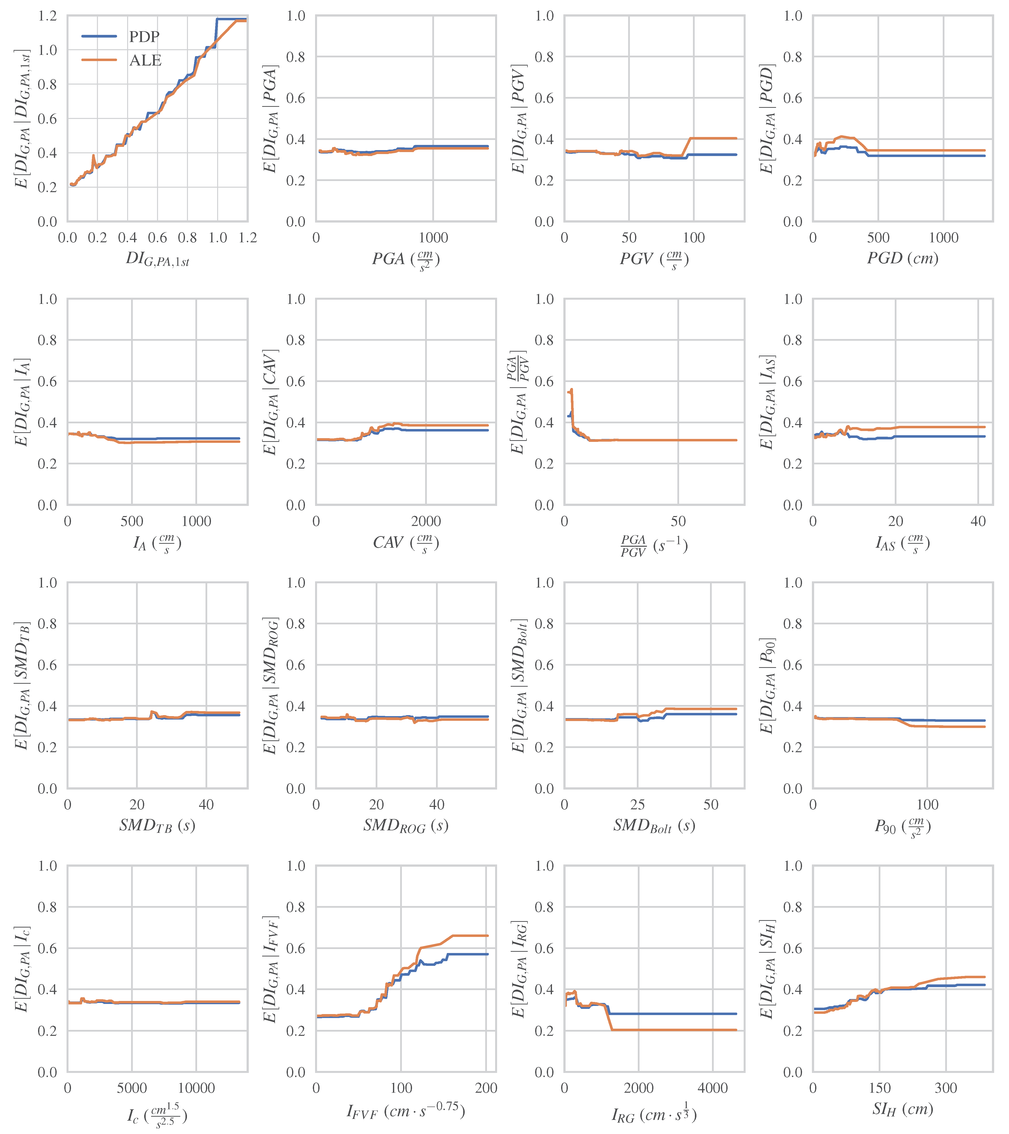
4.2.3. Global Explanation Methods (PDP and ALE)

Both PDPs and ALE, as global model-agnostic interpretation methods, can describe the general trends of our ML model with respect to input variables and depict the relationship between the cumulative seismic damage and a group of relevant predictors.

Figure 13 summarizes both PDPs and ALE results for the majority of the damage predictors. In each subplot, the y-axis depicts the expected value of the dependent variable, which in our case is the final damage ($\mathrm{D}{\mathrm{I}}_{\mathrm{G},\mathrm{P}\mathrm{A}}$), while the x-axis represents the value of the examined damage predictor. The positive impact of the initial damage on the final damage across its entire range of values can be observed. There is a sharp increase to the point where the initial damage takes value equal to unit. Beyond that, the trend levels off horizontally. ${\mathrm{I}}_{\mathrm{F}\mathrm{V}\mathrm{F}}$ has a positive impact for values between 50 and 150 cm·s${}^{-0.75}$, and zero impact for smaller and larger values. The corresponding final damage ranges from 0.25 to 0.56 by PDP and 0.25 to 0.65 by ALE. As observed, a larger cumulative damage range affected by ${\mathrm{I}}_{\mathrm{F}\mathrm{V}\mathrm{F}}$ is identified by ALE. $\mathrm{S}{\mathrm{I}}_{\mathrm{H}}$ has a notable positive impact on the final damage for values ranging from 80 to 180 cm. Moreover, final damage values falling between 0.3 and 0.45 appear to be influenced by this parameter. Subsequently, values of $\frac{\mathrm{P}\mathrm{G}\mathrm{A}}{\mathrm{P}\mathrm{G}\mathrm{V}}$ smaller than 15 ${\mathrm{s}}^{-1}$ appear to have a negative impact on the final damages and larger values present zero impact. $\mathrm{C}\mathrm{A}\mathrm{V}$ has an increasing outcome in the interval of 500–1500 $\frac{\mathrm{c}\mathrm{m}}{\mathrm{s}}$, increasing the damage from 0.3 to 0.4, and zero effect outside of this range. ${\mathrm{I}}_{\mathrm{R}\mathrm{G}}$ appears to have a predominantly negative influence on damage in the range of [0.2, 0.4]. Other seismic parameters ($\mathrm{P}\mathrm{G}\mathrm{D}$, $\mathrm{P}\mathrm{G}\mathrm{V}$, ${\mathrm{I}}_{\mathrm{A}\mathrm{S}}$, $\mathrm{P}\mathrm{G}\mathrm{A}$, $\mathrm{S}\mathrm{M}{\mathrm{D}}_{\mathrm{B}\mathrm{o}\mathrm{l}\mathrm{t}}$, ${\mathrm{I}}_{\mathrm{A}}$) seem to have less influence on shaping the final damage, affecting its values between 0.3 and 0.4. All the other input parameters appear to have very small or zero impact on the prediction of final damage, predicting values around 0.33, which is the mean output of our total sample. As a general observation, ALE indicates wider ranges of the dependent variable affected in comparison with PDP for every input feature.

In summary, this section explored the interpretability of the devised ML model by discussing feature importances, local explanation methods (LIME and SHAP), and global explanation methods (PDP and ALE). The results showed that initial damage, ${\mathrm{I}}_{\mathrm{F}\mathrm{V}\mathrm{F}}$, and $\mathrm{S}{\mathrm{I}}_{\mathrm{H}}$ are among the most crucial predictors of the final damage. Additionally, the local explanation methods provided insights into the positive or negative influence of each input variable on the cumulative seismic damage, while the global explanation methods described the general trends of the ML model with respect to damage predictors.

5. Conclusions

In this study, interpretable ML models to estimate the cumulative damage of an eight-story RC frame subjected to earthquake sequences were presented and analysed. Through the application of local and global explanation methods, a more profound understanding of the impact of individual features and their interactions in the context of ultimate seismic damage was achieved. Local explanation techniques, LIME and SHAP, delivered in-depth insights into how each feature influences the prediction on an individual level, while global explanation approaches, PDP and ALE, facilitated the comprehension of the general trends of the ML model concerning input variables. The utilization of these interpretation methodologies contributes to the creation of more transparent and interpretable models, which is of paramount importance for the implementation of ML methods in earthquake engineering problems. Our research investigated the accumulation of damage during a sequence of earthquakes, identifying crucial predictors and understanding their impact on the final damage ($\mathrm{D}{\mathrm{I}}_{\mathrm{G},\mathrm{P}\mathrm{A}}$). The input variables for the regression problem were divided into two distinct physical classes: pre-existing damage from the initial seismic event and the characteristics of the subsequent ground motion expressed using the Park and Ang damage index ($\mathrm{D}{\mathrm{I}}_{\mathrm{G},\mathrm{P}\mathrm{A},1\mathrm{s}\mathrm{t}}$) and 16 Intensity Measures (IMs), respectively.

The main outcomes are:

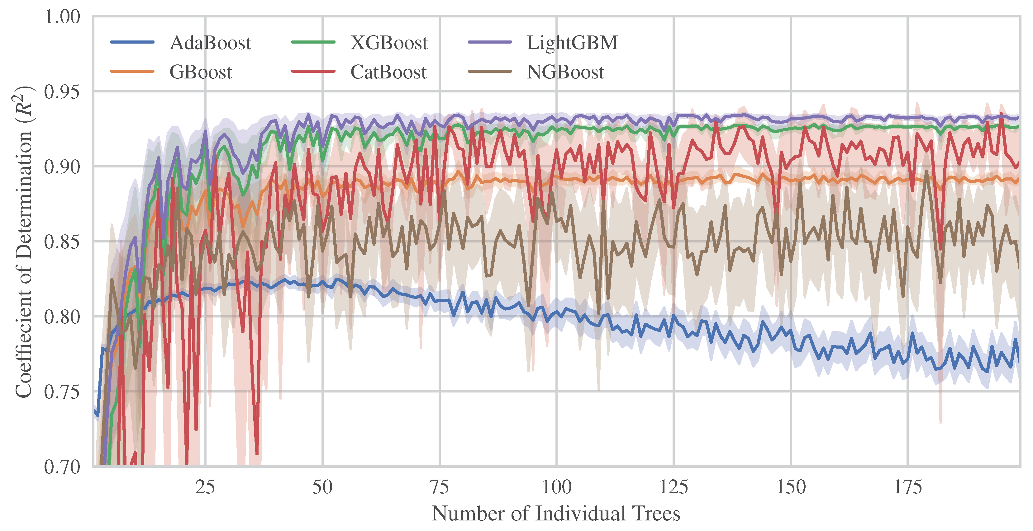
• The most efficient model for predicting final structural damage under seismic sequences was an instance of the LightGBM method with an ${\mathrm{R}}^2$ greater than 0.95, while the method with the poorest performance was KNN, with an ${\mathrm{R}}^2$ value of approximately 0.4.
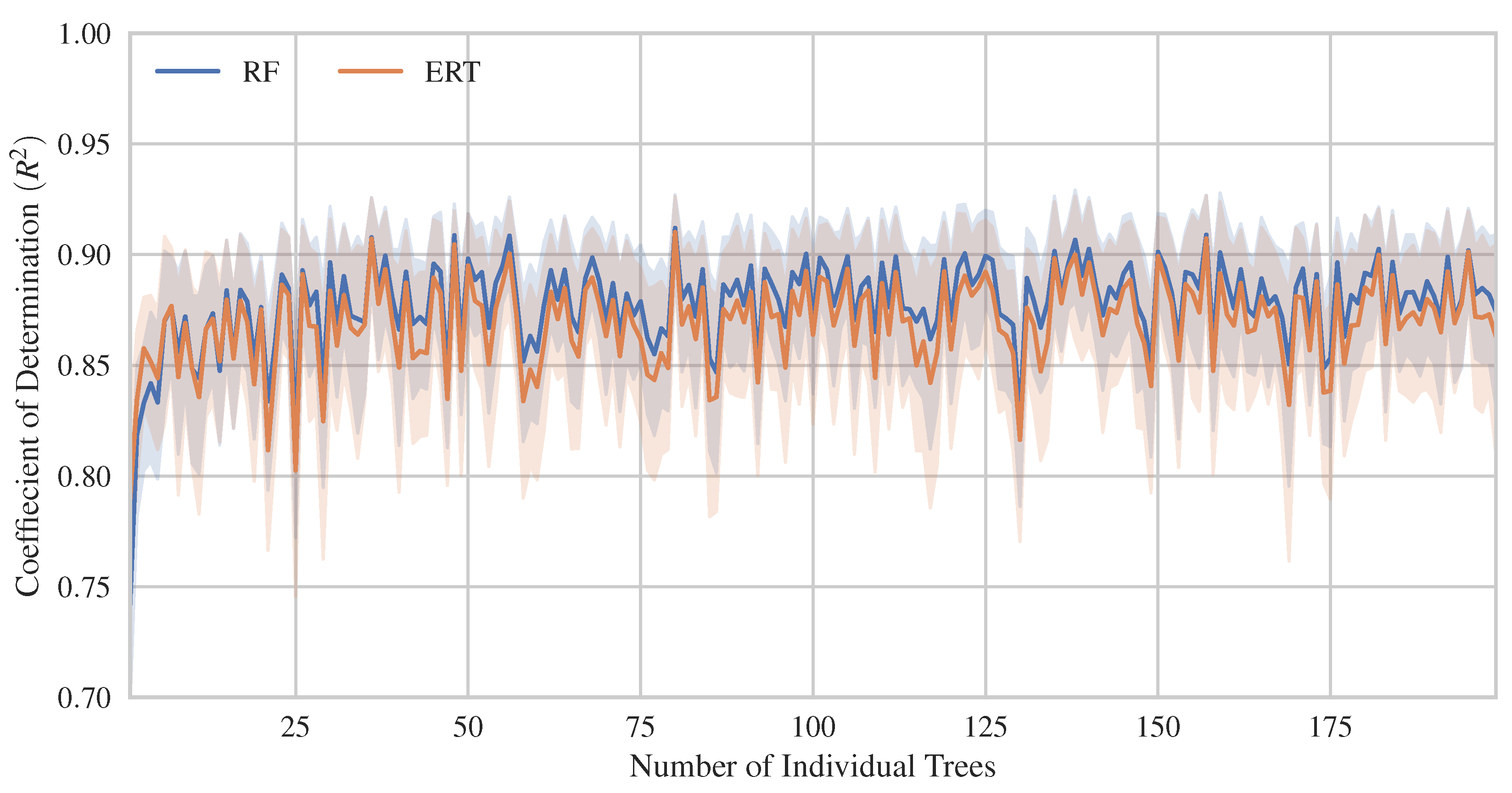
• Among the examined boosted trees, LightGBM and XGBoost demonstrated the most optimized and robust performance even against small changes in their hyperparameters. Moreover, they present great resistance to overfitting as the number of trees increases.
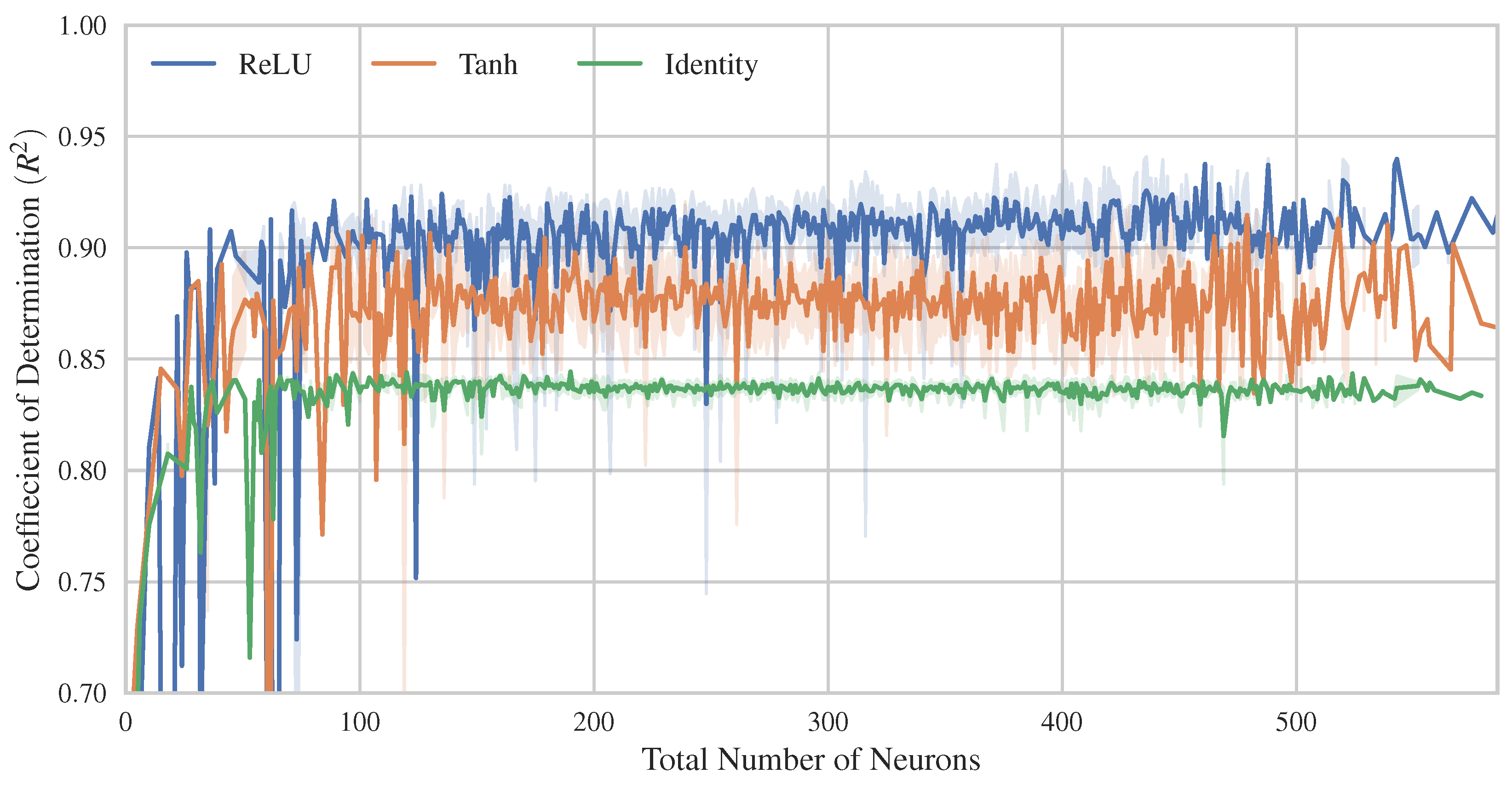
• In the case of Multi-Layer Perceptrons (MLPs), the ReLU activation function appeared to yield better performance, followed by the Tanh activation function. In addition, the MLP model presents slightly better bias-variance balance than the other advanced ML models.
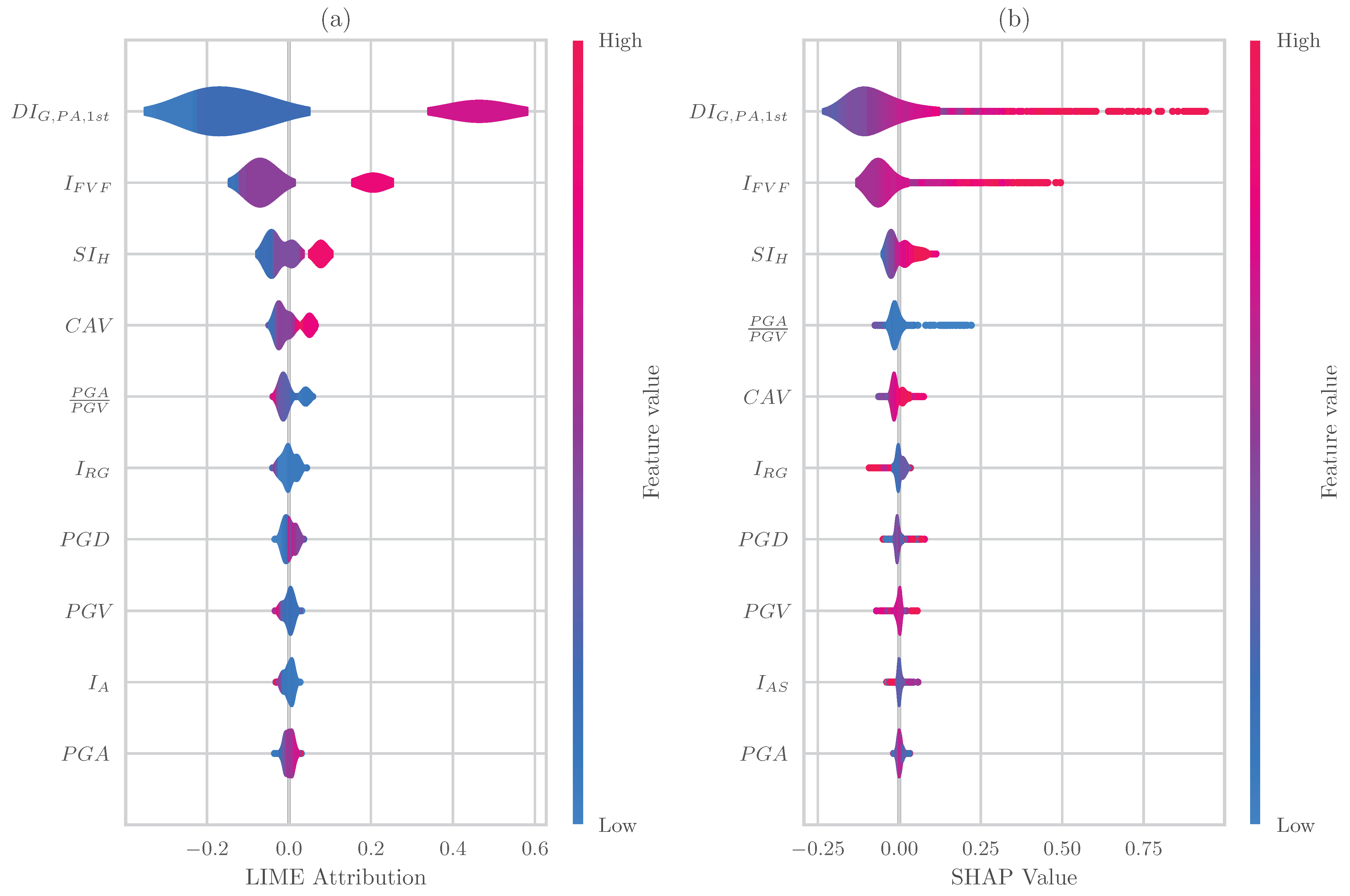
• All the interpretation methods identified the initial damage $\mathrm{D}{\mathrm{I}}_{\mathrm{G},\mathrm{P}\mathrm{A},1\mathrm{s}\mathrm{t}}$ as the most significant feature followed by the IMs of the subsequent seismic shock. However, the ranking of the IMs importance is varying between the adopted approaches. The majority of interpretation methods indicate the ${\mathrm{I}}_{\mathrm{F}\mathrm{V}\mathrm{F}}$ as the most important IM, except for the impurity-based explanation, which identified $\mathrm{S}{\mathrm{I}}_{\mathrm{H}}$. As the second most important IM, LIME and SHAP ranked $\mathrm{S}{\mathrm{I}}_{\mathrm{H}}$, although permutation ranked $\frac{\mathrm{P}\mathrm{G}\mathrm{A}}{\mathrm{P}\mathrm{G}\mathrm{V}}$, and impurity ranked ${\mathrm{I}}_{\mathrm{A}\mathrm{S}}$.
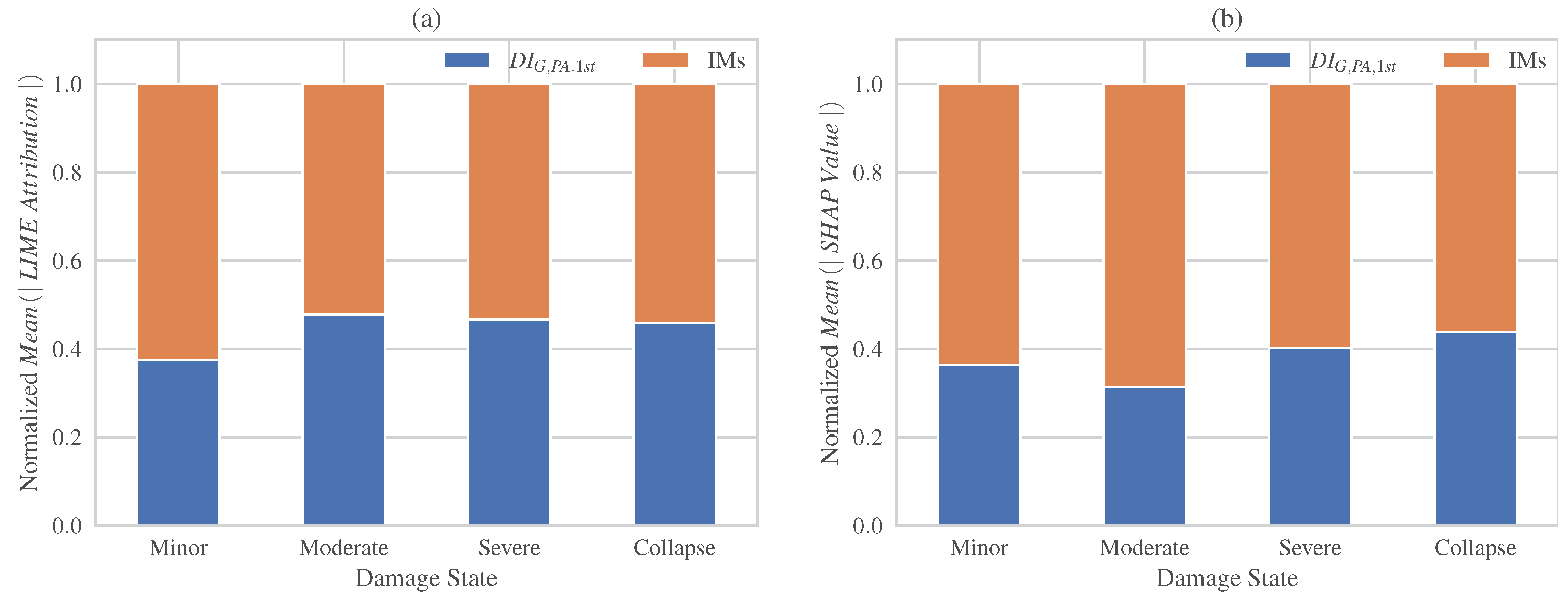
• In case of examining the effect of all the IMs in total, both LIME and SHAP local explanation methods show that the contribution of the subsequent ground motion is larger than that of initial damage $\mathrm{D}{\mathrm{I}}_{\mathrm{G},\mathrm{P}\mathrm{A},1\mathrm{s}\mathrm{t}}$. In general, the effect of the initial damage tends to increase as the final increases. However, they differ in their estimation of contributions for higher damage states.
• The analysis of PDPs and ALE reveals key insights into the effects of damage predictors on the final damage. The pre-existing damage demonstrates a positive influence across the entire range of cumulative damage. Additionally, ${\mathrm{I}}_{\mathrm{F}\mathrm{V}\mathrm{F}}$ and $\mathrm{S}{\mathrm{I}}_{\mathrm{H}}$ present a notable positive impact on moderate final damages. In contrast, $\frac{\mathrm{P}\mathrm{G}\mathrm{A}}{\mathrm{P}\mathrm{G}\mathrm{V}}$ values smaller than 15 ${\mathrm{s}}^{-1}$ seems to have a negative impact on moderate final damages, while $\mathrm{C}\mathrm{A}\mathrm{V}$ and ${\mathrm{I}}_{\mathrm{R}\mathrm{G}}$ demonstrate more complex effects in a narrower range of the final damage.

An important direction identified for future research is the extension of the approach presented in this study to encompass different building types. While robust findings were yielded from the current study, which focused on an eight-story RC frame, it is understood that seismic responses could vary among different building typologies, thus leading to distinct damage patterns. As such, it is recommended that a range of structural configurations, from low-rise to high-rise buildings, should be incorporated in future studies. Moreover, it is of utmost significance to take into consideration structures with irregularities in plan or height, as well as the effects of dual structural systems and infill walls. Furthermore, future investigations are encouraged to consider variations in construction detailing and materials. In addition, the inclusion of real-world instances could become a major target area. The aim is to verify the reliability and validity of our current modelling effort, which could be accomplished through such applications.

References

1. Atwater, B.F. Evidence for great Holocene earthquakes along the outer coast of Washington State. Science 1987, 236, 942–944. [Google Scholar] [CrossRef] [PubMed]
2. Plafker, G.; Savage, J.C. Mechanism of the Chilean earthquakes of 21 and 22 May 1960. Geol. Soc. Am. Bull. 1970, 81, 1001–1030. [Google Scholar] [CrossRef]
3. Chiaraluce, L.; Di Stefano, R.; Tinti, E.; Scognamiglio, L.; Michele, M.; Casarotti, E.; Cattaneo, M.; De Gori, P.; Chiarabba, C.; Monachesi, G.; et al. The 2016 central Italy seismic sequence: A first look at the mainshocks, aftershocks, and source models. Seismol. Res. Lett. 2017, 88, 757–771. [Google Scholar] [CrossRef]
4. Gatti, M. Peak horizontal vibrations from GPS response spectra in the epicentral areas of the 2016 earthquake in central Italy. Geomat. Nat. Hazards Risk 2018, 9, 403–415. [Google Scholar] [CrossRef]
5. Brandenberg, S.J.; Wang, P.; Nweke, C.C.; Hudson, K.; Mazzoni, S.; Bozorgnia, Y.; Hudnut, K.W.; Davis, C.A.; Ahdi, S.K.; Zareian, F.; et al. Preliminary Report on Engineering and Geological Effects of the July 2019 Ridgecrest Earthquake Sequence; Technical Report; Geotechnical Extreme Event Reconnaissance Association: Berkeley, CA, USA, 2019. [Google Scholar] [CrossRef]
6. Naddaf, M. Turkey-Syria earthquake: What scientists know. Nature 2023, 614, 398–399. [Google Scholar] [CrossRef]
7. İlki, A.; Demir, C.; Goksu, C.; Sarı, B. A brief outline of February 6, 2023 Earthquakes (M7.8-M7.7) in Türkiye with a focus on performance/failure of structures. In Proceedings of the Workshop on Innovative Seismic Protection of Structural Elements and Structures with Novel Materials, Civil Engineering Department (DUTh), Xanthi, Greece, 24 February 2023; Available online: https://drive.google.com/file/d/1acQRyrNnHlba87xAdTI3iUHBphFEAbIx/view (accessed on 15 March 2023).
8. Abdelnaby, A. Multiple Earthquake Effects on Degrading Reinforced Concrete Structures. Ph.D. Thesis, University of Illinois at Urbana-Champaign, Urbana and Champaign, IL, USA, 2012. [Google Scholar]
9. Hatzivassiliou, M.; Hatzigeorgiou, G.D. Seismic sequence effects on three-dimensional reinforced concrete buildings. Soil Dyn. Earthq. Eng. 2015, 72, 77–88. [Google Scholar] [CrossRef]
10. Kavvadias, I.E.; Rovithis, P.Z.; Vasiliadis, L.K.; Elenas, A. Effect of the aftershock intensity characteristics on the seismic response of RC frame buildings. In Proceedings of the 16th European Conference on Earthquake Engineering, Thessaloniki, Greece, 18–21 June 2018. [Google Scholar]
11. Trevlopoulos, K.; Guéguen, P. Period elongation-based framework for operative assessment of the variation of seismic vulnerability of reinforced concrete buildings during aftershock sequences. Soil Dyn. Earthq. Eng. 2016, 84, 224–237. [Google Scholar] [CrossRef]
12. Shokrabadi, M.; Burton, H.V.; Stewart, J.P. Impact of sequential ground motion pairing on mainshock-aftershock structural response and collapse performance assessment. J. Struct. Eng. 2018, 144, 04018177. [Google Scholar] [CrossRef]
13. Furtado, A.; Rodrigues, H.; Varum, H.; Arêde, A. Mainshock-aftershock damage assessment of infilled RC structures. Eng. Struct. 2018, 175, 645–660. [Google Scholar] [CrossRef]
14. Di Sarno, L.; Pugliese, F. Seismic fragility of existing RC buildings with corroded bars under earthquake sequences. Soil Dyn. Earthq. Eng. 2020, 134, 106169. [Google Scholar] [CrossRef]
15. Iervolino, I.; Chioccarelli, E.; Suzuki, A. Seismic damage accumulation in multiple mainshock–aftershock sequences. Earthq. Eng. Struct. Dyn. 2020, 49, 1007–1027. [Google Scholar] [CrossRef]
16. Rajabi, E.; Ghodrati Amiri, G. Behavior factor prediction equations for reinforced concrete frames under critical mainshock-aftershock sequences using artificial neural networks. Sustain. Resilient Infrastruct. 2021, 7, 552–567. [Google Scholar] [CrossRef]
17. Soureshjani, O.K.; Massumi, A. Seismic behavior of RC moment resisting structures with concrete shear wall under mainshock–aftershock seismic sequences. Bull. Earthq. Eng. 2022, 20, 1087–1114. [Google Scholar] [CrossRef]
18. Khansefid, A. An investigation of the structural nonlinearity effects on the building seismic risk assessment under mainshock–aftershock sequences in Tehran metro city. Adv. Struct. Eng. 2021, 24, 3788–3791. [Google Scholar] [CrossRef]
19. Hu, J.; Wen, W.; Zhai, C.; Pei, S.; Ji, D. Seismic resilience assessment of buildings considering the effects of mainshock and multiple aftershocks. J. Build. Eng. 2023, 68, 106110. [Google Scholar] [CrossRef]
20. Askouni, P.K. The Effect of Sequential Excitations on Asymmetrical Reinforced Concrete Low-Rise Framed Structures. Symmetry 2023, 15, 968. [Google Scholar] [CrossRef]
21. Zhao, J.; Ivan, J.N.; DeWolf, J.T. Structural damage detection using artificial neural networks. J. Infrastruct. Syst. 1998, 4, 93–101. [Google Scholar] [CrossRef]
22. Stavroulakis, G.E.; Antes, H. Nondestructive elastostatic identification of unilateral cracks through BEM and neural networks. Comput. Mech. 1997, 20, 439–451. [Google Scholar] [CrossRef]
23. De Lautour, O.R.; Omenzetter, P. Prediction of seismic-induced structural damage using artificial neural networks. Eng. Struct. 2009, 31, 600–606. [Google Scholar] [CrossRef]
24. Lagaros, N.D.; Papadrakakis, M. Neural network based prediction schemes of the non-linear seismic response of 3D buildings. Adv. Eng. Softw. 2012, 44, 92–115. [Google Scholar] [CrossRef]
25. Sánchez Silva, M.; García, L. Earthquake damage assessment based on fuzzy logic and neural networks. Earthq. Spectra 2001, 17, 89–112. [Google Scholar] [CrossRef]
26. Alvanitopoulos, P.; Andreadis, I.; Elenas, A. Neuro–fuzzy techniques for the classification of earthquake damages in buildings. Measurement 2010, 43, 797–809. [Google Scholar] [CrossRef]
27. Vrochidou, E.; Alvanitopoulos, P.F.; Andreadis, I.; Elenas, A. Intelligent systems for structural damage assessment. J. Intell. Syst. 2018, 29, 378–392. [Google Scholar] [CrossRef]
28. Mangalathu, S.; Sun, H.; Nweke, C.C.; Yi, Z.; Burton, H.V. Classifying earthquake damage to buildings using machine learning. Earthq. Spectra 2020, 36, 183–208. [Google Scholar] [CrossRef]
29. Wang, S.; Cheng, X.; Li, Y.; Song, X.; Guo, R.; Zhang, H.; Liang, Z. Rapid visual simulation of the progressive collapse of regular reinforced concrete frame structures based on machine learning and physics engine. Eng. Struct. 2023, 286, 116129. [Google Scholar] [CrossRef]
30. Wen, W.; Zhang, C.; Zhai, C. Rapid seismic response prediction of RC frames based on deep learning and limited building information. Eng. Struct. 2022, 267, 114638. [Google Scholar] [CrossRef]
31. Natarajan, Y.; Wadhwa, G.; Ranganathan, P.A.; Natarajan, K. Earthquake Damage Prediction and Rapid Assessment of Building Damage Using Deep Learning. In Proceedings of the 2023 International Conference on Advances in Electronics, Communication, Computing and Intelligent Information Systems (ICAECIS), Bengaluru, India, 19–21 April 2023; pp. 540–547. [Google Scholar] [CrossRef]
32. Sri Preethaa, K.; Munisamy, S.D.; Rajendran, A.; Muthuramalingam, A.; Natarajan, Y.; Yusuf Ali, A.A. Novel ANOVA-Statistic-Reduced Deep Fully Connected Neural Network for the Damage Grade Prediction of Post-Earthquake Buildings. Sensors 2023, 23, 6439. [Google Scholar] [CrossRef]
33. Zhang, R.; Liu, Y.; Sun, H. Physics-guided convolutional neural network (PhyCNN) for data-driven seismic response modeling. Eng. Struct. 2020, 215, 110704. [Google Scholar] [CrossRef]
34. Muradova, A.D.; Stavroulakis, G.E. Physics-informed neural networks for elastic plate problems with bending and Winkler-type contact effects. J. Serbian Soc. Comput. Mech. 2021, 15, 45–54. [Google Scholar] [CrossRef]
35. Katsikis, D.; Muradova, A.D.; Stavroulakis, G.E. A Gentle Introduction to Physics-Informed Neural Networks, with Applications in Static Rod and Beam Problems. J. Adv. Appl. Comput. Math. 2022, 9, 103–128. [Google Scholar] [CrossRef]
36. Morfidis, K.; Kostinakis, K. Seismic parameters’ combinations for the optimum prediction of the damage state of R/C buildings using neural networks. Adv. Eng. Softw. 2017, 106, 1–16. [Google Scholar] [CrossRef]
37. Hwang, S.H.; Mangalathu, S.; Shin, J.; Jeon, J.S. Machine learning-based approaches for seismic demand and collapse of ductile reinforced concrete building frames. J. Build. Eng. 2021, 34, 101905. [Google Scholar] [CrossRef]
38. Kalakonas, P.; Silva, V. Earthquake scenarios for building portfolios using artificial neural networks: Part I—Ground motion modelling. Bull. Earthq. Eng. 2022, 20, 1–22. [Google Scholar] [CrossRef]
39. Zhang, H.; Cheng, X.; Li, Y.; He, D.; Du, X. Rapid seismic damage state assessment of RC frames using machine learning methods. J. Build. Eng. 2022, 65, 105797. [Google Scholar] [CrossRef]
40. Yuan, X.; Chen, G.; Jiao, P.; Li, L.; Han, J.; Zhang, H. A neural network-based multivariate seismic classifier for simultaneous post-earthquake fragility estimation and damage classification. Eng. Struct. 2022, 255, 113918. [Google Scholar] [CrossRef]
41. Kazemi, P.; Ghisi, A.; Mariani, S. Classification of the Structural Behavior of Tall Buildings with a Diagrid Structure: A Machine Learning-Based Approach. Algorithms 2022, 15, 349. [Google Scholar] [CrossRef]
42. Karbassi, A.; Mohebi, B.; Rezaee, S.; Lestuzzi, P. Damage prediction for regular reinforced concrete buildings using the decision tree algorithm. Comp. Struct. 2014, 130, 46–56. [Google Scholar] [CrossRef]
43. Ghiasi, R.; Torkzadeh, P.; Noori, M. A machine-learning approach for structural damage detection using least square support vector machine based on a new combinational kernel function. Struct. Health Monit. 2016, 15, 302–316. [Google Scholar] [CrossRef]
44. Chen, S.Z.; Feng, D.C.; Wang, W.J.; Taciroglu, E. Probabilistic Machine-Learning Methods for Performance Prediction of Structure and Infrastructures through Natural Gradient Boosting. J. Struct. Eng. 2022, 148, 04022096. [Google Scholar] [CrossRef]
45. Jia, D.W.; Wu, Z.Y. Structural probabilistic seismic risk analysis and damage prediction based on artificial neural network. Structures 2022, 41, 982–996. [Google Scholar] [CrossRef]
46. Kiani, J.; Camp, C.; Pezeshk, S. On the application of machine learning techniques to derive seismic fragility curves. Comp. Struct. 2019, 218, 108–122. [Google Scholar] [CrossRef]
47. Kazemi, F.; Asgarkhani, N.; Jankowski, R. Machine learning-based seismic fragility and seismic vulnerability assessment of reinforced concrete structures. Soil Dyn. Earthq. Eng. 2023, 166, 107761. [Google Scholar] [CrossRef]
48. Dabiri, H.; Faramarzi, A.; Dall’Asta, A.; Tondi, E.; Micozzi, F. A machine learning-based analysis for predicting fragility curve parameters of buildings. J. Build. Eng. 2022, 62, 105367. [Google Scholar] [CrossRef]
49. Yang, J.; Zhuang, H.; Zhang, G.; Tang, B.; Xu, C. Seismic performance and fragility of two-story and three-span underground structures using a random forest model and a new damage description method. Tunn. Undergr. Space Technol. 2023, 135, 104980. [Google Scholar] [CrossRef]
50. De-Miguel-Rodríguez, J.; Morales-Esteban, A.; Requena-García-Cruz, M.; Zapico-Blanco, B.; Segovia-Verjel, M.; Romero-Sánchez, E.; Carvalho-Estêvão, J.M. Fast seismic assessment of built urban areas with the accuracy of mechanical methods using a feedforward neural network. Sustainability 2022, 14, 5274. [Google Scholar] [CrossRef]
51. Gravett, D.Z.; Mourlas, C.; Taljaard, V.L.; Bakas, N.; Markou, G.; Papadrakakis, M. New fundamental period formulae for soil-reinforced concrete structures interaction using machine learning algorithms and ANNs. Soil Dyn. Earthq. Eng. 2021, 144, 106656. [Google Scholar] [CrossRef]
52. Morfidis, K.; Stefanidou, S.; Markogiannaki, O. A Rapid Seismic Damage Assessment (RASDA) Tool for RC Buildings Based on an Artificial Intelligence Algorithm. Appl. Sci. 2023, 13, 5100. [Google Scholar] [CrossRef]
53. Lazaridis, P.C.; Kavvadias, I.E.; Demertzis, K.; Iliadis, L.; Papaleonidas, A.; Vasiliadis, L.K.; Elenas, A. Structural Damage Prediction Under Seismic Sequence Using Neural Networks. In Proceedings of the 8th International Conference on Computational Methods in Structural Dynamics and Earthquake Engineering (COMPDYN 2021), Athens, Greece, 28–30 June 2021. [Google Scholar] [CrossRef]
54. Lazaridis, P.C.; Kavvadias, I.E.; Demertzis, K.; Iliadis, L.; Vasiliadis, L.K. Structural Damage Prediction of a Reinforced Concrete Frame under Single and Multiple Seismic Events Using Machine Learning Algorithms. Appl. Sci. 2022, 12, 3845. [Google Scholar] [CrossRef]
55. Sun, H.; Burton, H.V.; Huang, H. Machine Learning Applications for Building Structural Design and Performance Assessment: State-of-the-Art Review. J. Build. Eng. 2020, 33, 101816. [Google Scholar] [CrossRef]
56. Xie, Y.; Ebad Sichani, M.; Padgett, J.E.; DesRoches, R. The promise of implementing machine learning in earthquake engineering: A state-of-the-art review. Earthq. Spectra 2020, 36, 1769–1801. [Google Scholar] [CrossRef]
57. Harirchian, E.; Hosseini, S.E.A.; Jadhav, K.; Kumari, V.; Rasulzade, S.; Işık, E.; Wasif, M.; Lahmer, T. A Review on Application of Soft Computing Techniques for the Rapid Visual Safety Evaluation and Damage Classification of Existing Buildings. J. Build. Eng. 2021, 43, 102536. [Google Scholar] [CrossRef]
58. Sony, S.; Dunphy, K.; Sadhu, A.; Capretz, M. A systematic review of convolutional neural network-based structural condition assessment techniques. Eng. Struct. 2021, 226, 111347. [Google Scholar] [CrossRef]
59. Tapeh, A.T.G.; Naser, M. Artificial Intelligence, Machine Learning, and Deep Learning in Structural Engineering: A Scientometrics Review of Trends and Best Practices. Arch. Comput. Methods Eng. 2022, 30, 115–159. [Google Scholar] [CrossRef]
60. Thai, H.T. Machine learning for structural engineering: A state-of-the-art review. Structures 2022, 38, 448–491. [Google Scholar] [CrossRef]
61. You, Z. Intelligent construction: Unlocking opportunities for the digital transformation of China’s construction industry. Eng. Constr. Archit. Manag. 2022, 29, 326. [Google Scholar] [CrossRef]
62. Málaga-Chuquitaype, C. Machine learning in structural design: An opinionated review. Front. Built Environ. 2022, 8, 6. [Google Scholar] [CrossRef]
63. Demertzis, K.; Demertzis, S.; Iliadis, L. A Selective Survey Review of Computational Intelligence Applications in the Primary Subdomains of Civil Engineering Specializations. Appl. Sci. 2023, 13, 3380. [Google Scholar] [CrossRef]
64. Wang, C.; Song, L.H.; Yuan, Z.; Fan, J.S. State-of-the-Art AI-Based Computational Analysis in Civil Engineering. J. Ind. Inf. Integr. 2023, 2023, 100470. [Google Scholar] [CrossRef]
65. Zhou, Z.; Yu, X.; Lu, D. Identifying Optimal Intensity Measures for Predicting Damage Potential of Mainshock–Aftershock Sequences. Appl. Sci. 2020, 10, 6795. [Google Scholar] [CrossRef]
66. Amiri, S.; Di Sarno, L.; Garakaninezhad, A. Correlation between non-spectral and cumulative-based ground motion intensity measures and demands of structures under mainshock-aftershock seismic sequences considering the effects of incident angles. Structures 2022, 46, 1209–1223. [Google Scholar] [CrossRef]
67. Demertzis, K.; Kostinakis, K.; Morfidis, K.; Iliadis, L. An interpretable machine learning method for the prediction of R/C buildings’ seismic response. J. Build. Eng. 2022, 2022, 105493. [Google Scholar] [CrossRef]
68. Park, Y.J.; Ang, A.H.S. Mechanistic seismic damage model for reinforced concrete. J. Struct. Eng. 1985, 111, 722–739. [Google Scholar] [CrossRef]
69. Elenas, A. Interdependency between seismic acceleration parameters and the behaviour of structures. Soil Dyn. Earthq. Eng. 1997, 16, 317–322. [Google Scholar] [CrossRef]
70. Elenas, A.; Liolios, A.; Vasiliadis, L. Correlation Factors between Seismic Acceleration Parameters and Damage Indicators of Reinforced Concrete Structures; Balkema Publishers: Rotterdam, The Netherlands, 1999; Volume 2, pp. 1095–1100. [Google Scholar]
71. Elenas, A. Correlation between seismic acceleration parameters and overall structural damage indices of buildings. Soil Dyn. Earthq. Eng. 2000, 20, 93–100. [Google Scholar] [CrossRef]
72. Vrochidou, E.; Alvanitopoulos, P.; Andreadis, I.; Elenas, A. Correlation between seismic intensity parameters of HHT-based synthetic seismic accelerograms and damage indices of buildings. In Proceedings of the IFIP International Conference on Artificial Intelligence Applications and Innovations, Halkidiki, Greece, 27–30 September 2012; pp. 425–434. [Google Scholar] [CrossRef]
73. Fontara, I.; Athanatopoulou, A.; Avramidis, I. Correlation between advanced, structure-specific ground motion intensity measures and damage indices. In Proceedings of the 15th World Conference on Earthquake Engineering, Lisbon, Portugal, 24–28 September 2012; pp. 24–28. [Google Scholar]
74. Van Cao, V.; Ronagh, H.R. Correlation between seismic parameters of far-fault motions and damage indices of low-rise reinforced concrete frames. Soil Dyn. Earthq. Eng. 2014, 66, 102–112. [Google Scholar] [CrossRef]
75. Kostinakis, K.; Athanatopoulou, A.; Morfidis, K. Correlation between ground motion intensity measures and seismic damage of 3D R/C buildings. Eng. Struct. 2015, 82, 151–167. [Google Scholar] [CrossRef]
76. Lazaridis, P.C.; Kavvadias, I.E.; Vasiliadis, L.K. Correlation between Seismic Parameters and Damage Indices of Reinforced Concrete Structures. In Proceedings of the 4th Panhellenic Conference on Earthquake Engineering and Engineering Seismology, Athens, Greece, 5–7 September 2019. [Google Scholar]
77. Palanci, M.; Senel, S.M. Correlation of earthquake intensity measures and spectral displacement demands in building type structures. Soil Dyn. Earthq. Eng. 2019, 121, 306–326. [Google Scholar] [CrossRef]
78. Kramer, S.L. Geotechnical Earthquake Engineering; Prentice Hall: Upper Saddle River, NJ, USA, 1996. [Google Scholar]
79. Arias, A. A measure of earthquake intensity. In Seismic Design for Nuclear Power Plants; Massachusetts Institute of Technology: Cambridge, MA, USA, 1970. [Google Scholar]
80. Araya, R.; Saragoni, G.R. Earthquake accelerogram destructiveness potential factor. In Proceedings of the 8th World Conference on Earthquake Engineering, San Francisco, CA, USA, 11–18 July 1985; Volume 11, pp. 835–843. [Google Scholar]
81. Trifunac, M.D.; Brady, A.G. A study on the duration of strong earthquake ground motion. Bull. Seismol. Soc. Am. 1975, 65, 581–626. [Google Scholar]
82. Reinoso, E.; Ordaz, M.; Guerrero, R. Influence of strong ground-motion duration in seismic design of structures. In Proceedings of the 12th World Conference on Earthquake Engineering, Auckland, New Zealand, 30 January–4 February 2000; Volume 1151. [Google Scholar]
83. Bolt, B.A. Duration of strong ground motion. In Proceedings of the 5th World Conference on Earthquake Engineering, Rome, Italy, 25–29 June 1973; Volume 292, pp. 25–29. [Google Scholar]
84. Fajfar, P.; Vidic, T.; Fischinger, M. A measure of earthquake motion capacity to damage medium-period structures. Soil Dyn. Earthq. Eng. 1990, 9, 236–242. [Google Scholar] [CrossRef]
85. Riddell, R.; Garcia, J.E. Hysteretic energy spectrum and damage control. Earthq. Eng. Struct. Dyn. 2001, 30, 1791–1816. [Google Scholar] [CrossRef]
86. Housner, G.W. Spectrum intensities of strong-motion earthquakes. In Proceedings of the Symposium on Earthquake and Blast Effects on Structures, Los Angeles, CA, USA, 25–29 June 1952. [Google Scholar]
87. Husid, R. Características de terremotos. Análisis general. Revista IDIEM 1969, 8, ág-21. [Google Scholar]
88. Kunnath, S.K.; Reinhorn, A.M.; Lobo, R. IDARC Version 3.0: A Program for the Inelastic Damage Analysis of Reinforced Concrete Structures; Technical report; US National Center for Earthquake Engineering Research (NCEER), University at Buffalo 212: Ketter Hall Buffalo, NY, USA, 1992; pp. 14260–14300. [Google Scholar]
89. Karabini, M.A.; Karabinis, A.J.; Karayannis, C.G. Seismic characteristics of a Π-shaped 4-story RC structure with open ground floor. Earthq. Struct. 2022, 22, 345. [Google Scholar] [CrossRef]
90. Park, Y.J.; Ang, A.H.; Wen, Y.K. Damage-limiting aseismic design of buildings. Earthq. Spectra 1987, 3, 1585416. [Google Scholar] [CrossRef]
91. Hatzigeorgiou, G.D.; Liolios, A.A. Nonlinear behaviour of RC frames under repeated strong ground motions. Soil Dyn. Earthq. Eng. 2010, 30, 1010–1025. [Google Scholar] [CrossRef]
92. CEN. Eurocode 8: Design of Structures for Earthquake Resistance-Part 1: General Rules, Seismic Actions and Rules for Buildings; European Committee for Standardization: Brussels, Belgium, 2005. [Google Scholar]
93. Chalioris, C.E. Analytical model for the torsional behaviour of reinforced concrete beams retrofitted with FRP materials. Eng. Struct. 2007, 29, 3263–3276. [Google Scholar] [CrossRef]
94. Bantilas, K.E.; Kavvadias, I.E.; Vasiliadis, L.K. Capacity spectrum method based on inelastic spectra for high viscous damped buildings. Earthq. Struct. 2017, 13, 337–351. [Google Scholar] [CrossRef]
95. Anagnostou, E.; Rousakis, T.C.; Karabinis, A.I. Seismic retrofitting of damaged RC columns with lap-spliced bars using FRP sheets. Compos. Part B Eng. 2019, 166, 598–612. [Google Scholar] [CrossRef]
96. Thomoglou, A.K.; Rousakis, T.C.; Achillopoulou, D.V.; Karabinis, A.I. Ultimate shear strength prediction model for unreinforced masonry retrofitted externally with textile reinforced mortar. Earthq. Struct. 2020, 19, 411–425. [Google Scholar] [CrossRef]
97. Rousakis, T.; Anagnostou, E.; Fanaradelli, T. Advanced Composite Retrofit of RC Columns and Frames with Prior Damages—Pseudodynamic Finite Element Analyses and Design Approaches. Fibers 2021, 9, 56. [Google Scholar] [CrossRef]
98. Karabini, M.; Rousakis, T.; Golias, E.; Karayannis, C. Seismic Tests of Full Scale Reinforced Concrete T Joints with Light External Continuous Composite Rope Strengthening—Joint Deterioration and Failure Assessment. Materials 2023, 16, 2718. [Google Scholar] [CrossRef]
99. Valles, R.; Reinhorn, A.M.; Kunnath, S.K.; Li, C.; Madan, A. IDARC2D Version 4.0: A Computer Program for the Inelastic Damage Analysis of Buildings; Technical Report; US National Center for Earthquake Engineering Research (NCEER), University at Buffalo 212: Ketter Hall Buffalo, NY, USA, 1996; pp. 14260–14300. [Google Scholar]
100. Park, Y.J.; Reinhorn, A.M.; Kunnath, S.K. IDARC: Inelastic Damage Analysis of Reinforced Concrete Frame–Shear–Wall Structures; National Center for Earthquake Engineering Research Buffalo, University at Buffalo 212: Ketter Hall Buffalo, NY, USA, 1987; pp. 14260–14300. [Google Scholar]
101. Eaton, J.W. GNU Octave and reproducible research. J. Process Control 2012, 22, 1433–1438. [Google Scholar] [CrossRef]
102. Eaton, J.W.; Bateman, D.; Hauberg, S.; Wehbring, R. GNU Octave Version 6.1.0 Manual: A High-Level Interactive Language for Numerical Computations; Free Software Foundation: Bostoin, MA, USA, 2020. [Google Scholar]
103. Luzi, L.; Lanzano, G.; Felicetta, C.; D’Amico, M.; Russo, E.; Sgobba, S.; Pacor, F.; ORFEUS Working Group 5. Engineering Strong Motion Database (ESM) (Version 2.0); Istituto Nazionale di Geofisica e Vulcanologia (INGV): Rome, Italy, 2020. [Google Scholar] [CrossRef]
104. Goulet, C.A.; Kishida, T.; Ancheta, T.D.; Cramer, C.H.; Darragh, R.B.; Silva, W.J.; Hashash, Y.M.; Harmon, J.; Stewart, J.P.; Wooddell, K.E.; et al. PEER NGA-East Database; Technical Report; Pacific Earthquake Engineering Research Center: Berkeley, CA, USA, 2014. [Google Scholar]
105. Van Rossum, G. Python Reference Manual; National Research Institute for Mathematics and Computer Science, Netherlands Organisation for Scientific Research: Amsterdam, The Netherlands, 1995. [Google Scholar]
106. Harris, C.R.; Millman, K.J.; Van der Walt, S.J.; Gommers, R.; Virtanen, P.; Cournapeau, D.; Wieser, E.; Taylor, J.; Berg, S.; Smith, N.J.; et al. Array programming with NumPy. Nature 2020, 585, 357–362. [Google Scholar] [CrossRef]
107. Papazafeiropoulos, G.; Plevris, V. OpenSeismoMatlab: A new open-source software for strong ground motion data processing. Heliyon 2018, 4, e00784. [Google Scholar] [CrossRef] [PubMed]
108. Galton, F. Regression towards mediocrity in hereditary stature. J. Anthropol. Inst. Great Br. Irel. 1886, 15, 246–263. [Google Scholar] [CrossRef]
109. Stanton, J.M. Galton, Pearson, and the peas: A brief history of linear regression for statistics instructors. J. Stat. Educ. 2001, 9, 1–13. [Google Scholar] [CrossRef]
110. Tibshirani, R. Regression shrinkage and selection via the lasso. J. R. Stat. Soc. Ser. B 1996, 58, 267–288. [Google Scholar] [CrossRef]
111. Hoerl, A.E.; Kennard, R.W. Ridge regression: Biased estimation for nonorthogonal problems. Technometrics 1970, 12, 55–67. [Google Scholar] [CrossRef]
112. Zou, H.; Hastie, T. Regularization and variable selection via the elastic net. J. R. Stat. Soc. Ser. B 2005, 67, 301–320. [Google Scholar] [CrossRef]
113. Altman, N.S. An introduction to kernel and nearest-neighbor nonparametric regression. Am. Stat. 1992, 46, 175–185. [Google Scholar] [CrossRef]
114. Breiman, L.; Friedman, J.H.; Olshen, R.A.; Stone, C.J. Classification and Regression Trees; Routledge: London, UK, 2017. [Google Scholar] [CrossRef]
115. Breiman, L. Random forests. Mach. Learn. 2001, 45, 5–32. [Google Scholar] [CrossRef]
116. Friedman, J.H. Greedy function approximation: A gradient boosting machine. Ann. Stat. 2001, 1, 1189–1232. [Google Scholar] [CrossRef]
117. Geurts, P.; Ernst, D.; Wehenkel, L. Extremely randomized trees. Mach. Learn. 2006, 63, 3–42. [Google Scholar] [CrossRef]
118. Freund, Y.; Schapire, R.E. A decision-theoretic generalization of on-line learning and an application to boosting. J. Comput. Syst. Sci. 1997, 55, 119–139. [Google Scholar] [CrossRef]
119. Drucker, H. Improving regressors using boosting techniques. In Proceedings of the 14th International Conference on Machine Learning (ICML), Nashville, TN, USA, 8–12 July 1997; Volume 97, pp. 107–115. [Google Scholar]
120. Ke, G.; Meng, Q.; Finley, T.; Wang, T.; Chen, W.; Ma, W.; Ye, Q.; Liu, T.Y. LightGBM: A Highly Efficient Gradient Boosting Decision Tree. In Proceedings of the Advances in Neural Information Processing Systems (NIPS), Long Beach, CA, USA, 4–9 December 2017; Guyon, I., Luxburg, U.V., Bengio, S., Wallach, H., Fergus, R., Vishwanathan, S., Garnett, R., Eds.; Curran Associates Inc.: Red Hook, NY, USA, 2017; Volume 30. [Google Scholar]
121. Dorogush, A.V.; Ershov, V.; Gulin, A. CatBoost: Gradient boosting with categorical features support. In Proceedings of the Workshop on ML Systems at NIPS, Long Beach, CA, USA, 8 December 2017. [Google Scholar]
122. Prokhorenkova, L.; Gusev, G.; Vorobev, A.; Dorogush, A.V.; Gulin, A. CatBoost: Unbiased boosting with categorical features. In Proceedings of the Advances in Neural Information Processing Systems (NeurIPS), Montréal, QC, Canada, 3–8 December 2018; Bengio, S., Wallach, H., Larochelle, H., Grauman, K., Cesa Bianchi, N., Garnett, R., Eds.; Curran Associates Inc.: Red Hook, NY, USA, 2018; Volume 31. [Google Scholar]
123. Chen, T.; Guestrin, C. XGBoost: A Scalable Tree Boosting System. In Proceedings of the 22nd ACM SIGKDD International Conference on Knowledge Discovery and Data Mining, San Francisco, CA, USA, 13–17 August 2016; pp. 785–794. [Google Scholar] [CrossRef]
124. Duan, T.; Anand, A.; Ding, D.Y.; Thai, K.K.; Basu, S.; Ng, A.; Schuler, A. NGBoost: Natural Gradient Boosting for Probabilistic Prediction. In Proceedings of the 37th International Conference on Machine Learning (ICML), Virtual, 13–18 July 2020; Daumé, H., Singh, A., Eds.; Curran Associates Inc.: Red Hook, NY, USA, 2020; Volume 119, pp. 2690–2700. [Google Scholar]
125. Rojas, R. Neural Networks: A Systematic Introduction; Springer Science & Business Media: Berlin/Heidelberg, Germany, 1996. [Google Scholar] [CrossRef]
126. Minsky, M.; Papert, S.A. Perceptrons: An Introduction to Computational Geometry; MIT Press: Cambridge, MA, USA, 2017. [Google Scholar]
127. Goodfellow, I.; Bengio, Y.; Courville, A. Deep Learning; MIT Press: Cambridge, MA, USA, 2016; Available online: http://www.deeplearningbook.org (accessed on 15 March 2023).
128. Rumelhart, D.E.; Hinton, G.E.; Williams, R.J. Learning representations by back-propagating errors. Nature 1986, 323, 533–536. [Google Scholar] [CrossRef]
129. LeCun, Y.A.; Bottou, L.; Orr, G.B.; Müller, K.R. Efficient backprop. In Neural Networks: Tricks of the Trade; Springer: Berlin/Heidelberg, Germany, 2012; pp. 9–48. [Google Scholar] [CrossRef]
130. Bergstra, J.; Bardenet, R.; Bengio, Y.; Kégl, B. Algorithms for Hyper-Parameter Optimization. In Proceedings of the Advances in Neural Information Processing Systems (NIPS), Granada, Spain, 12–15 December 2011; Shawe Taylor, J., Zemel, R., Bartlett, P., Pereira, F., Weinberger, K., Eds.; Curran Associates Inc.: Red Hook, NY, USA, 2011; Volume 24. [Google Scholar]
131. Bergstra, J.; Bengio, Y. Random search for hyper-parameter optimization. J. Mach. Learn. Res. 2012, 13, 281–305. [Google Scholar]
132. Picard, R.R.; Cook, R.D. Cross-validation of regression models. J. Am. Stat. Assoc. 1984, 79, 575–583. [Google Scholar] [CrossRef]
133. Pedregosa, F.; Varoquaux, G.; Gramfort, A.; Michel, V.; Thirion, B.; Grisel, O.; Blondel, M.; Prettenhofer, P.; Weiss, R.; Dubourg, V.; et al. Scikit-learn: Machine Learning in Python. J. Mach. Learn. Res. 2011, 12, 2825–2830. [Google Scholar]
134. Lei, M.; Lin, D.; Huang, Q.; Shi, C.; Huang, L. Research on the construction risk control technology of shield tunnel underneath an operational railway in sand pebble formation: A case study. Eur. J. Environ. Civ. Eng. 2020, 24, 1558–1572. [Google Scholar] [CrossRef]
135. Huang, L.; Huang, S.; Lai, Z. On the optimization of site investigation programs using centroidal Voronoi tessellation and random field theory. Comput. Geotech. 2020, 118, 103331. [Google Scholar] [CrossRef]
136. Lin, Y.; Ma, J.; Lai, Z.; Huang, L.; Lei, M. A FDEM approach to study mechanical and fracturing responses of geo-materials with high inclusion contents using a novel reconstruction strategy. Eng. Fract. Mech. 2023, 282, 109171. [Google Scholar] [CrossRef]
137. Lin, Y.; Yin, Z.Y.; Wang, X.; Huang, L. A systematic 3D simulation method for geomaterials with block inclusions from image recognition to fracturing modelling. Theor. Appl. Fract. Mech. 2022, 117, 103194. [Google Scholar] [CrossRef]
138. Ma, J.; Chen, J.; Guan, J.; Lin, Y.; Chen, W.; Huang, L. Implementation of Johnson-Holmquist-Beissel model in four-dimensional lattice spring model and its application in projectile penetration. Int. J. Impact Eng. 2022, 170, 104340. [Google Scholar] [CrossRef]
139. Ding, W.; Jia, S. An Improved Equation for the Bearing Capacity of Concrete-Filled Steel Tube Concrete Short Columns Based on GPR. Buildings 2023, 13, 1226. [Google Scholar] [CrossRef]
140. Molnar, C. Interpretable Machine Learning—A Guide for Making Black Box Models Explainable, 2nd ed.; Independently Published; 2023; Available online: https://christophm.github.io/interpretable-ml-book (accessed on 15 March 2023).
141. Mangalathu, S.; Karthikeyan, K.; Feng, D.C.; Jeon, J.S. Machine-learning interpretability techniques for seismic performance assessment of infrastructure systems. Eng. Struct. 2022, 250, 112883. [Google Scholar] [CrossRef]
142. Wakjira, T.G.; Ibrahim, M.; Ebead, U.; Alam, M.S. Explainable machine learning model and reliability analysis for flexural capacity prediction of RC beams strengthened in flexure with FRCM. Eng. Struct. 2022, 255, 113903. [Google Scholar] [CrossRef]
143. Junda, E.; Málaga-Chuquitaype, C.; Chawgien, K. Interpretable machine learning models for the estimation of seismic drifts in CLT buildings. J. Build. Eng. 2023, 2023, 106365. [Google Scholar] [CrossRef]
144. Hastie, T.; Friedman, J.H.; Tibshirani, R. The Elements of Statistical Learning: Data Mining, Inference, and Prediction; Springer: New York, NY, USA, 2009; Volume 2. [Google Scholar] [CrossRef]
145. Apley, D.W.; Zhu, J. Visualizing the effects of predictor variables in black box supervised learning models. J. R. Stat. Soc. Ser. B 2020, 82, 1059–1086. [Google Scholar] [CrossRef]
146. Ribeiro, M.T.; Singh, S.; Guestrin, C. “Why Should I Trust You?”: Explaining the Predictions of Any Classifier. In Proceedings of the 22nd ACM SIGKDD International Conference on Knowledge Discovery and Data Mining, San Francisco, CA, USA, 13–17 August 2016; pp. 1135–1144. [Google Scholar] [CrossRef]
147. Lundberg, S.M.; Lee, S.I. A Unified Approach to Interpreting Model Predictions. In Proceedings of the 31st Conference on Neural Information Processing Systems (NIPS 2017), Long Beach, CA, USA, 4–9 December 2017; Guyon, I., Luxburg, U.V., Bengio, S., Wallach, H., Fergus, R., Vishwanathan, S., Garnett, R., Eds.; Curran Associates Inc.: Red Hook, NY, USA, 2017; pp. 4765–4774. [Google Scholar]
148. Shapley, L.S. A value for n-person games. Ann. Math. Stud. 1953, 28, 307–317. [Google Scholar]
Figure 1. Indicative seismic signal comprising two successive ground motions and the accompanying evolution of seismic damage.
Sustainability 15 12768 g001
Figure 2. (a) The examined RC frame [54], (b) concrete and (c) steel stress-strain rules, (d) the implemented hysteretic rule.
Sustainability 15 12768 g002
Figure 3. (a) The machine learning workflow followed in this study and (b) the K-fold CV schematic representation.
Sustainability 15 12768 g003
Figure 4. A comprehensive visualization of the ML methods and the interpretation techniques used in this study.
Sustainability 15 12768 g004
Figure 5. Side-by-side bar plot comparing the performance of different ML methods on training (10-fold), CV (10-fold), and test sets.
Sustainability 15 12768 g005
Figure 6. The evolution of R 2 versus the number of base learner trees for boosted trees.
Sustainability 15 12768 g006
Figure 7. The evolution of R 2 versus the number of base learner trees for random forest algorithms.
Sustainability 15 12768 g007
Figure 8. The evolution of R 2 versus the total number of neurons, for each activation function.
Sustainability 15 12768 g008
Figure 9. Feature importances for the ML methods with R 2 > 0.9 , according to the permutation method.
Sustainability 15 12768 g009
Figure 10. Feature importances for the best LightGBM model, using different interpretation methods.
Sustainability 15 12768 g010
Figure 11. Violin plots represent the distribution of (a) LIME attributions (b) SHAP values.
Sustainability 15 12768 g011
Figure 12. Stacked bar plot of grouped (a) LIME attributions (b) SHAP values for IMs and D I G , P A , normalized to unity.
Sustainability 15 12768 g012
Figure 13. The expected value of D I G , P A with respect to each examined input feature, according to the PDP and ALE methods.
Sustainability 15 12768 g013