Article

Monitoring Intertidal Habitats for Effects from Biosolids Applications onto an Adjacent Forestry Plantation

1
Cawthron Institute, Nelson 7010, New Zealand
2
Nelson Regional Sewerage Business Unit, Nelson 7010, New Zealand
*
Author to whom correspondence should be addressed.
Current address: Jacobs, Christchurch 8013, New Zealand.
Current address: MacLean Marine Identifiers Ltd., Nelson 7010, New Zealand.
Sustainability 2023, 15(16), 12279; https://doi.org/10.3390/su151612279
Submission received: 6 May 2023 / Revised: 7 August 2023 / Accepted: 8 August 2023 / Published: 11 August 2023
(This article belongs to the Special Issue Sustainable Waste Management and Utilization)

Abstract

:
Stabilised organic solids derived from sewage sludge (“biosolids”) are applied to land as an alternative to disposal as landfill. This study evaluated the long-term effects of biosolids applied to forestry plantations on the adjacent intertidal habitats of Rabbit Island (New Zealand). On this island, biosolids are applied to enhance the growth of trees (Pinus radiata). Shoreline topography, macroalgal cover, sediment grain size, the concentrations of nutrients, trace metals, and faecal indicator bacteria, and benthic infaunal communities were studied in 2008, 2014, and 2019 at twelve intertidal transect sites (four “reference” and eight “application”) adjacent to forestry blocks where biosolids have been applied over a period of 24 years. The sediment composition did not differ significantly between the survey years or between the reference and application sites. Total nitrogen concentrations in the sediments increased over time at some transects, but such increases were not consistent among the application transects. No symptoms of excessive algal growth, sediment anoxia, and hydrogen sulphide odours were observed at most sites. Key infaunal taxa were similar between the reference and application transects. Overall, no long-term adverse changes to intertidal habitats attributed to biosolids application were detected between the reference and application sites. This study shows that biosolids application can co-occur without detectable adverse effects on nearby intertidal environments. In a global context of rising concern over climate change, environmental pollution, and resource scarcity, forest fertilisation with biosolids can facilitate biomass production and soil development while protecting valued coastal ecosystems.

1. Introduction

Biosolids (stabilised organic solids derived from sewage treatment processes) have been applied to land in an environmentally safe and cost-effective manner in many countries [1]. In Aotearoa New Zealand (NZ), this practice has been encouraged in many areas as a way of reducing the volume of waste diverted to landfills while improving soil properties and plant growth [2]. When applied to forestry plantations, biosolids can amend the soil by improving soil texture and providing nutrients (especially nitrogen and phosphorus; both frequently limited in forest soils) [3]. In the short-term, biosolids supply additional nutrients (e.g., nitrogen, phosphorus, magnesium, potassium) in an available form needed for plant growth. Biosolids are also a cost-effective alternative to chemical fertilisers.
Land application of biosolids can cause negative effects on soils, surface water, and groundwater. This is particularly so when application rates of inorganic (e.g., trace metals/metalloids, nutrients), organic (e.g., pesticides, pharmaceuticals), and microbial contaminants in the biosolids exceed the retention capacity of soils and vegetation [1,4]. Contaminants in surface water and groundwater may potentially adversely affect the sediments and fauna of adjacent marine (including intertidal) areas. The likely mechanism of the effect is the transfer of organic and inorganic nutrients and other contaminants in the biosolids from percolating through the shallow soil layer and, to a lesser extent, direct surface runoff during rainfall periods [5,6]. However, the occurrence of these contaminants in the biosolids does not necessarily mean that there is a risk to the environment or human health. Metal chemistry and bioavailability in biosolid-amended soils is controlled by the properties of the biosolids and soils [7].
The impact of biosolids applications on the physical, chemical, and biological properties of soils in forestry areas has been studied [8,9], but the impacts on nearby intertidal environments have not been studied. In NZ, repeated applications of biosolids to forestry plantations on low-fertility, sandy soils were shown to improve soil fertility, tree nutrition, and pine productivity (up to 34% increase in tree stem volumes relative to control sites reported in one study) [8]. In the same study area, biosolids applications were found to alter soil microbial activity, biomass, and composition and, consequently, to influence nitrogen mineralisation rates in the soil [9]. Good practice guidelines and risk assessments for the treatment and beneficial use of biosolids on land have been developed in many countries (e.g., the United States of America, Canada, Australia, the United Kingdom, several European Union Member States), including Aotearoa (New Zealand) [10,11]. New Zealand’s guidelines recognise the potential for biosolids to contaminate watercourses and affect biodiversity, particularly when biosolids are applied shortly after rainfall events or on waterlogged or steeply sloping land [11]. While the effects of biosolids application on soil properties [9,12], nutrient balance [13], and tree growth [3,14,15,16] are well characterised, few studies have investigated the long-term effects of biosolids applications on adjacent coastal environments of high ecological and cultural value.
Domestic and industrial wastewater from the towns of Nelson and Richmond, in the north of the South Island of NZ, is treated at the Bell Island Wastewater Treatment Plant (WWTP). The volume of wastewater currently treated is equivalent to that generated by a population of 105,000 people [17]. At the WWTP, waste activated sludge is thickened, blended with primary sludge, and fed to an autothermal anaerobic digestion process. The digestion process stabilises and pasteurises the biosolids so that they can be applied to land as soil additives and fertilisers with no restriction and in compliance with the contaminant limits prescribed in the New Zealand Biosolids Guidelines (Grade Ab standards, i.e., meets the stabilisation levels for pathogen reduction and strict standards for heavy metals and organic compounds) [10,18]. Biosolids from the plant have been applied to promote the growth of radiata (Monterey) pine (Pinus radiata) in forestry blocks on nearby Moturoa/Rabbit Island (“the Island”; Figure 1) since 1997. Biosolids are applied to these areas because the sandy soils are deficient in nutrients and organic matter [19,20].
Despite their beneficial uses, biosolids can contain substances harmful to the environment and human health. These include inorganic contaminants (e.g., metals and other trace elements), organic contaminants (e.g., polychlorinated biphenyls, dioxins, pharmaceuticals, and surfactants), microplastics, endocrine-disrupting chemicals, and pathogens (e.g., bacteria, viruses, and eggs of parasitic worms). For example, typical concentrations of trace metals in biosolids from the Bell Island WWTP are cadmium 3.1 mg/kg, chromium 103 mg/kg, copper 533 mg/kg, lead 50 mg/kg, mercury 1.1 mg/kg, nickel 48 mg/kg, and zinc 1020 mg/kg [21]. However, the simple occurrence of contaminants in biosolids does not necessarily mean that they pose a risk to public health or the environment. The chemical and biological compositions of biosolids vary with the composition of the wastewater entering the WWTP and the treatment processes employed.
Long-term monitoring is essential to inform any assessment of environmental risks from biosolids application areas that impinge on coastal habitats. The aim of this study was to evaluate data from three consecutive surveys (2008, 2014, and 2019) to identify any long-term adverse effects of biosolids application on the intertidal habitats adjacent to forestry blocks. These three surveys were part of a longer monitoring programme (1996–present). The study comprised surveys of shore topography and habitat types, sediment grain size, concentrations of organic matter, nitrogen, trace metals/metalloids, microalgae and macroalgae, infaunal and epifaunal community composition, and faecal indicator bacteria (FIB) contamination of shellfish. The hypothesis was that the transfer of nutrients (specifically nitrogen) and contaminants (specifically metals/metalloids and FIB) from biosolids to intertidal areas adjacent to the application areas via groundwater flow would alter their concentrations in intertidal sediments and, thereby, alter habitat quality and biota.

2. Materials and Methods
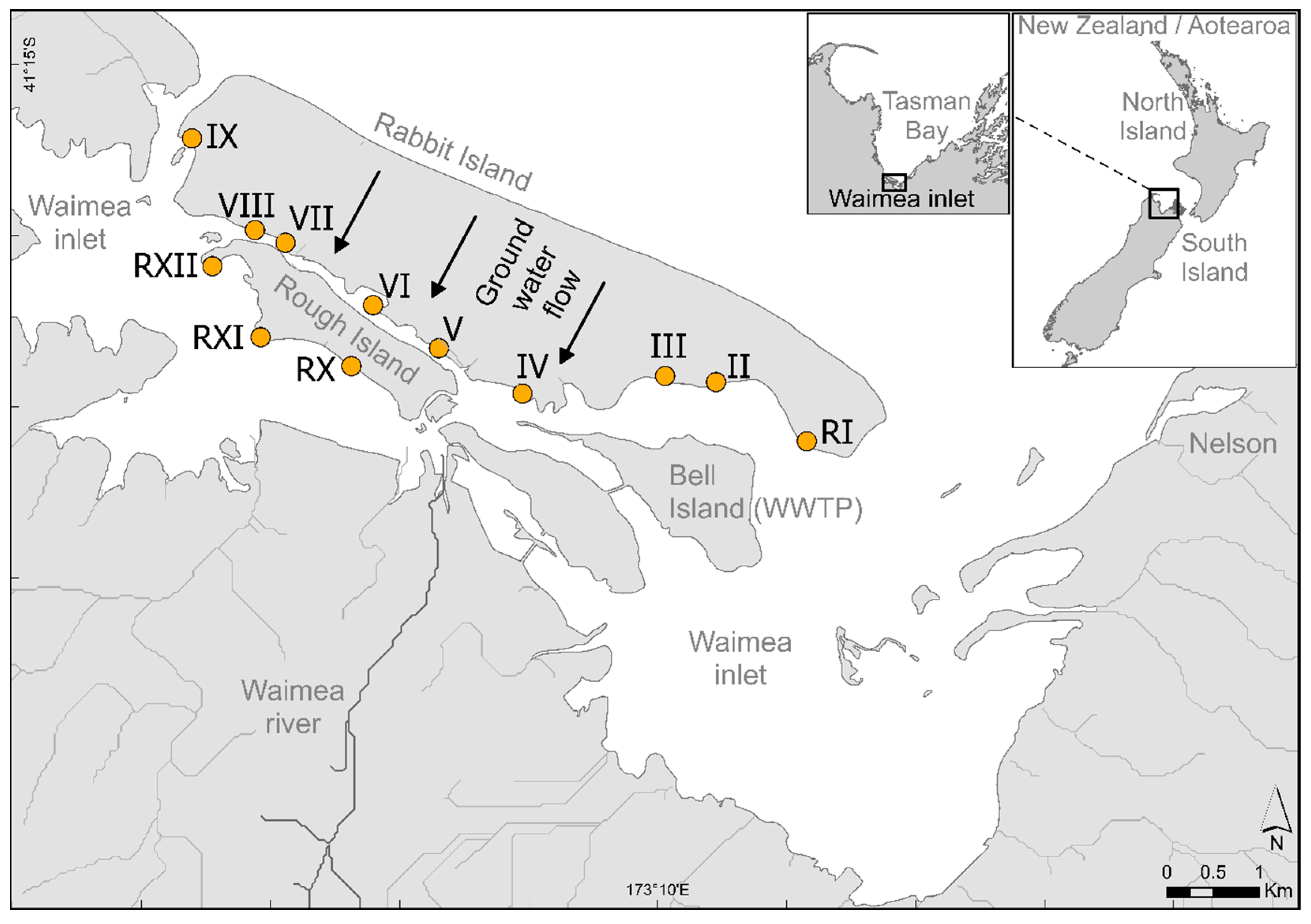
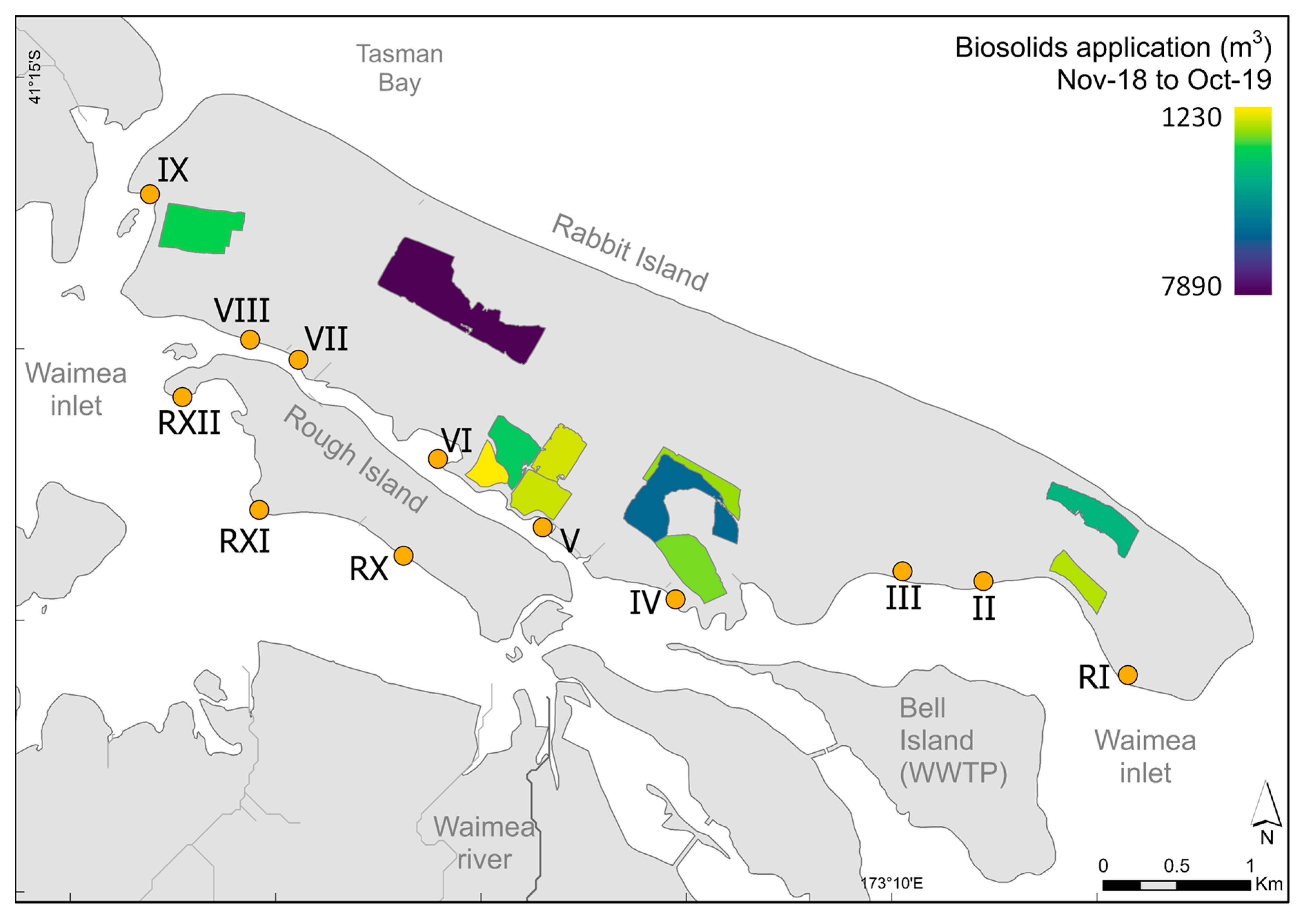
2.1. Study Area

Moturoa/Rabbit Island lies across the southernmost part of Tasman Bay, adjacent to the city of Nelson, on the South Island of NZ (Figure 1). The Island runs east–west for approximately 8 km and covers a total area of approximately 15 km2. South of the Island lies Waimea Inlet, a large and shallow (mean depth ≈ 1–2 m at high water), bar-built estuary. Waimea Inlet is one of the largest in NZ, with approximately 3300 ha of intertidal area and 600 ha of subtidal area [22,23,24]. The Inlet opens to Tasman Bay at the western and eastern ends of the Island (Figure 1). The spring tidal range is 3.7 m [25], and the residence time of the water ranges from 0.6 days (near complete tidal mixing) to 11.6 days [26]. The volumes of freshwater discharges to the Inlet from streams and rivers are low compared to the volumes of water exchanged by the tides. The main freshwater discharge to the Inlet is from the Waimea River and its tributaries (mean annual flow is 27.5 m3/s) [27].
The shores of the Island contain a wide variety of intertidal habitats, including soft muds, firm muddy sands, firm mobile sands, saltmarsh, seagrass, cobble and gravel fields, and Pacific oyster (Crassostrea gigas) and cockle (Austrovenus stutchburyi) beds [28]. Waimea Inlet has nationally significant ecosystem values [29]. It is an area of international importance for migratory bird species and a nursery and feeding ground for a diversity of invertebrate and fish species. However, given its proximity to urban and industrial areas, it is considered the most-threatened estuary in the Nelson/Marlborough region [22]. In addition to commercial forestry, the perimeter of the Island is used for various recreational activities, including walking, swimming, cycling, and horse riding.

2.2. Biosolids Application on Moturoa/Rabbit Island

Digested biosolids, consisting of 4% solid materials and 96% water by volume [21], are pumped from the WWTP to storage tanks at the Biosolids Application Facility on the Island and transported to forestry blocks in tankers, where they are applied via customised heavy-duty travelling irrigators [30]. Biosolids application occurs periodically throughout the year. Where required, restrictions are put in place on public access to certain forestry areas, and no application occurs near recreational areas [30]. Application is also prohibited within 15 m of the edge of the forest or within 50 m from the mean high water of spring tides, whichever is greater. Biosolids are normally applied post-harvest and prior to replanting of pine trees [29]. The long-term relationships between nitrogen/phosphorus availability and microbial activity in soils and tree biomass and composition following repeated application of biosolids have been studied on Rabbit Island [8,9]. The application rates are dependent on biosolids quality (particularly its nitrogen content), weather conditions (no application during wet weather or when wind promotes transport to sensitive receptors), tree age, and the limits imposed by the discharge permit conditions. The volume of biosolids applied to forestry blocks on the Island during the period 1997–2019, reflecting a gradual increase since 2003, is shown in Figure S1.

2.3. Coastal Monitoring Programme

The data analysed in this study were collected during environmental monitoring (required by regulatory authorities) to document any significant environmental effects of the biosolids application on the adjacent intertidal habitats of the Island. The monitoring programme had three components:
  • Qualitative surveys of substratum type, topography, and major biological habitats along transects perpendicular to the shoreline at six-month intervals for the first five years (1996–2001) of the application programme;
  • Quantitative transect surveys of benthic microalgal and macroalgal cover (in 1996, prior to application, and in 2003, 2008, 2014, and 2019);
  • Quantitative transect surveys of epifaunal organisms and burrows, infauna community composition (from 2008), visual assessment of the sediment profile (colour, depth of apparent redox discontinuity), sediment grain size, organic matter and nutrient content, and trace metal and bacteriological contamination along the foreshore (in 1996, prior to biosolids application (nutrients and organic matter only), and in 2003, 2008, 2014, and 2019).
This study presents the results of the 1996 pre-biosolids survey and compares the results of a subset of three consecutive surveys (2008, 2014, and 2019) representing a period of an increasing volume of biosolids applied (Figure S1).

2.3.1. Sampling Sites

Twelve intertidal transect locations were identified in the pre-application survey in 1996 (Figure 1). Transect locations were chosen to take into account the biosolids’ application areas, the predominant direction of groundwater flows, the efficiency of tidal flushing in the Inlet, and ecological information available for the study area [31,32]. The transects were located on the southern side of the Island (Figure 1), extending perpendicular to the shore from approximately spring high water to mean low water. Transects II, III, IV, V, VI, VII, VIII, and IX are adjacent to designated biosolids’ application areas, while Transects (R)I, (R)X, (R)XI, and (R)XII are adjacent to non-application areas, thus serving as “reference” transects.
The transects were set up as follows: a measuring tape extending from the transect marker (upper end) through the lower intertidal levels was used to relate shore characteristics to the position on the transect line; two monitoring sites, designated A (mid-transect) and B (lower transect), were situated at points where groundwater seepage was visually most apparent. Only one site was selected on Transect (R)X (mid-transect) because of its shorter length.

2.3.2. Field Observations

Changes in substrate type, shore topography, and major biological habitats along each transect were described in general terms. The site characteristics recorded were as follows:
  • Shoreline topography (description of surface features within the general transect vicinity, e.g., oyster reefs, macroalgal beds, tidal channels);
  • Sediment type (mud, sand, shell, etc.);
  • Abundance of conspicuous epifauna on five replicates 0.1 m2 quadrats (e.g., crab holes, shellfish, and other macroinvertebrate species);
  • Macroalgal species and percent coverage: Where a high level of macroalgal cover existed, the percent coverage of the sediment habitat was estimated using five replicates of a randomly placed 0.25 m2 quadrat containing gridlines, dividing it into 36 equally spaced squares. The number of grid intersections (including the outer frame) that overlapped vegetation were counted and the result converted to percent (i.e., number × 2 = %);
  • Sediment profiles (62 mm-diameter, 100 mm-depth cores extruded and described according to the stratification of colour and composition and any corresponding indications of sediment anoxia);
  • Obvious signs of organic or nutrient enrichment (e.g., hydrogen sulphide odours, bacterial or microalgal mat development) (see [33,34] for details of microalgal species identification).

2.3.3. Sediment, Infauna, and Shellfish Sampling

Three composite sediment samples were collected per site. Each composite comprised the top 1 cm of sediment from five replicate circles (0.0135 m2) randomly positioned within 10 m of the site marker (the top 1 cm was assumed to represent the depth to which most epibiota and infauna are exposed). The composite samples were thoroughly mixed in resealable bags and retained to determine total nitrogen (TN) content. Equal portions of the three composite samples were mixed in a separate resealable bag and retained to determine sediment grain size distribution and total organic content (as ash-free dry weight (AFDW)) (method details in Supplementary Materials). Equal portions of the two samples in the bag (i.e., those from the A and B sites for the same transect) were mixed in another resealable bag and used for the analysis of metals/metalloids. The samples were kept on ice while in the field. Upon returning to the laboratory, samples were either stored at 3 °C (particle size and organic content analyses) or −18 °C (remaining chemical analyses) until required for processing. Sediment infaunal samples were collected at the transect A and B sites by inserting a 131 mm-diameter core to a depth of at least 100 mm into the sediment. The contents of three replicate cores were gently washed through a 0.5 mm mesh sieve attached to one end of the core tube, and the residual material from each was preserved with a solution containing 95% ethanol with 5% glyoxal (as a fixative).
One sample of shellfish (cockles A. stutchburyi or Pacific oysters C. gigas) was collected by hand within the vicinity of each transect in sufficient numbers, depending on the size of the individuals, to provide enough flesh weight (at least 50 g) to accommodate the analytical requirements. These samples were put into resealable bags and kept on ice while in the field. Upon returning to the laboratory, transect composites were refrigerated for analyses of FIB (within 24 h) and frozen for subsequent analyses of trace metals/metalloids. Where benthic microalgal mats were visually obvious, they were collected from the sediment surface into a plastic container for microscopic identification of primary taxa in the laboratory [33,34].

2.3.4. Laboratory Analyses

The initial composite sediment samples were analysed for TN [35]. The mixed composites were analysed for grain size by wet sieving and AFDW by combustion at 500 °C (Reference [36] is cited in the Supplementary Materials). CAB composites were analysed for arsenic (As), cadmium (Cd), chromium (Cr), copper (Cu), lead (Pb), mercury (Hg), nickel (Ni), and zinc (Zn) by ICPMS after nitric/hydrochloric acid digestion (reference [37] is cited in the Supplementary Materials). Infauna were identified under a binocular microscope to the lowest practical taxa. Shellfish tissue samples were analysed for FIB (enterococci and Escherichia coli) by standard methods [38,39]. For identification of microalgae, sediment samples were homogenised, and 10 mL was dispensed into Utermöhl chambers. The samples were allowed to settle for 4 h before identification of the dominant and subdominant microalgae species to the genus level using an inverted microscope under bright field. Details of the nutrient, chemical, and microbiological testing methods are listed in Table S1 as the Supplementary Materials to this paper.

2.4. Data Analyses

Concentrations of TN are plotted as a function of distance from the nearest biosolids application area using data for 2018–2019. Volumes of biosolids applied to individual forestry blocks for this period were supplied as Excel files by Nelson Marlborough Waste Ltd (Nelson, Aotearoa New Zealand). Concentrations of As and metals were compared with default guideline values (DGVs) and guideline value-high (GV-High) [40]. Exceedance of these guidelines indicates that adverse ecological effects are likely to occur. The DGV indicates the concentration above which adverse effects on aquatic life are possible, while GV-high indicates concentrations at which such effects are probable.
Differences in sediment compositions between survey years and between the application and reference sites were analysed using Kruskal–Wallis and Mann–Whitney tests, respectively. Concentrations of E. coli in shellfish were compared with the standard for “Approved” shellfish-growing areas of the Regulated Control Scheme for Bivalve Molluscan Shellfish [41].
Benthic infaunal community structure (using aligned datasets between the years) was compared between survey sites (e.g., application vs. reference) and over time using indices and multivariate techniques. The indices used were species richness (SR) (the number of taxa), total abundance of individuals, measurements of evenness (Pielou’s J’) [42], and diversity (Shannon–Wiener’s H’ based on natural logs). For each index, statistical differences between the application and reference sites for each year were analysed using Mann–Whitney tests (pooled data). Average abundances of taxa contributing the highest percentages (>70%) to the dissimilarity between the application and reference stations were also compared for each survey year using the SIMPER routine (based on square-root-transformed data). Non-metric multidimensional scaling (MDS) was used to identify patterns in the community structure between survey sites (e.g., reference vs. application) and over time. For this, the data were run on a Bray–Curtis dissimilarity matrix based on square-root-transformed data [43]. All multivariate infaunal analyses and the calculation of the index values were performed using PRIMER v7 [44].

3. Results

3.1. Shoreline Observations

Visual inspection of the 12 monitoring sites between 2008 and 2019 recorded changes in habitat characteristics, in particular shore erosion, at several transects. This appeared to be attributable to natural coastal dynamics and/or logging activities occurring on the Island and unrelated to biosolids application. The evidence of erosion was particularly obvious where the top of the shore consisted of steep banks, leaving pine tree roots exposed and either suspended or collapsed on the beach, notably at Site III (application). In 2014, an increase in sediment deposition was recorded at Site VIII (application), possibly storm-related, resulting in the raised elevation and reduced tidal inundation of the shore.
Past forestry logging and associated vehicle disturbances had impacted the area around Application Sites V and VI, with the deposition of terrestrial vegetation debris (mainly from pine trees) in the intertidal area. This debris gradually disintegrated and was much reduced by 2014. Between 2008 and 2019, tidal flushing of the area between Moturoa/Rabbit Island and Rough Island was improved by the removal of a causeway at the western end of the channel between the islands. Subsequent erosion diminished the salt marsh vegetation (Salicornia (Sarcocornia) quinqueflora, Juncus kraussii) around it (Application Sites V and VI) and caused the shoreline to migrate landward at these transects.
Changes were seen over the study period in the beds of Pacific oysters along parts of the channel shore. Oyster numbers increased at Site VII (application), attributable to the removal of the causeway, resulting in more-efficient tidal flushing.
There is groundwater seepage along the perimeter of most of the study area, observed as diffuse large wet patches of sand in bands parallel to the shore rather than distinct discharge points. In the 2014 survey, salinity tests at Site VII indicated significant groundwater seepage (data not presented).
Most survey sites did not show obvious visual signs of nutrient enrichment (microalgal or macroalgal mats, sediment anoxia) during the monitoring period, with sediment cores relatively well oxygenated and with little or no macroalgal cover present on the sediment surface (Table 1). Signs of enrichment were noted at some transects (including reference ones) in the 2019 survey, evidenced by relatively high macroalgal cover and/or potential anoxia in the sediment profiles at Sites IIA, VIB (application), and (R)XIA. However, none of the cores had noticeable hydrogen sulphide odours.
Macroalgal cover was <9% at all sites in 2008 (Table 1). Cover was higher at some sites in 2014 (36% and 13% at Application Transects VII and IX, 19% at Reference Transect (R)XII) and higher again in 2019 (80%, 87%, 75%, and 35% at Application Transects V, VI, VII, and IX and 33%, 34%, and 32% at Reference Transects (R)X, (R)XI, and (R)XII). The dominant taxa were generally from the genus Ulva, either in blade (cf. Ulva pertusa) or filamentous (cf. Ulva compressa/Ulva intestinalis) forms. The red macroalga Agarophyton (Gracilaria) chilense was the dominant taxon at Transects VI and VII in 2008 (cover was <5% in 2008, having been higher in previous surveys), but had disappeared at Transect VII in 2014, replaced by Gelidium spp. (36% average cover), possibly in response to improved flushing after removal of the causeway. In 2019, A. chilense was the dominant red macroalga at Transect V (maximum average cover 73%). Although the highest values were at the application sites, the distribution of relatively high macroalgal cover among the transects did not suggest any clear effect of biosolids application.
Thin patches of the microalga Euglena sp. were observed at Transect II (application) in the 2003 survey. Visible dark-green mats comprised largely of the cyanobacterium Microcoleus (Phormidium) sp. were noted at Transect VIII (application) in the 2019 survey along the shoreline at 16–18 m from the high-water mark. Subdominant taxa within the mats were another cyanobacterium, Oscillatoria sp. and diatoms. No visually obvious microalgal or cyanobacteria mats were recorded at any other surveys/transects during the study.

3.2. Sediment Composition, Nitrogen and Contaminant Concentrations, and Benthic Communities

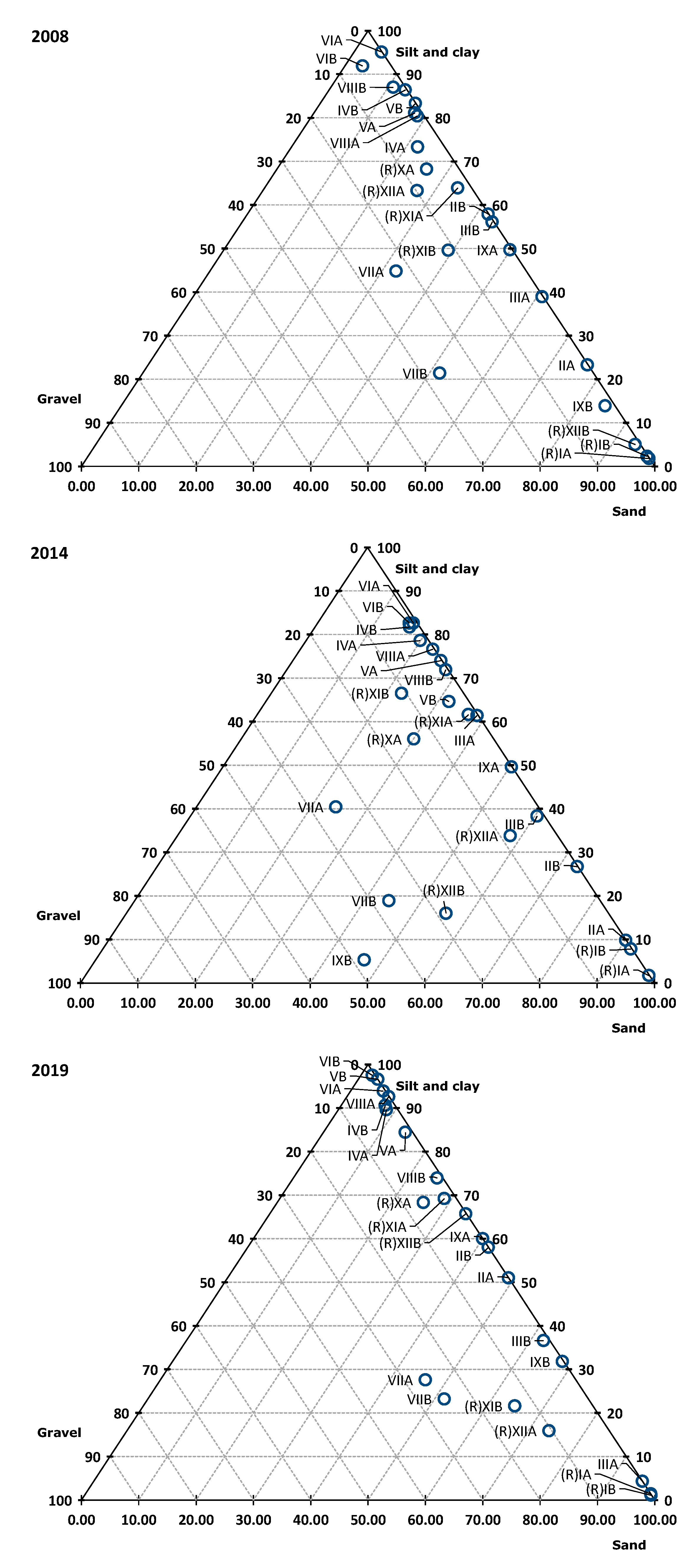
3.2.1. Sediment Composition

Transects IV, V, VI, and VIII (application) were dominated by silt and clay (>70%), while Transects II, III, and VII (application) had greater proportions of sand and gravel (Figure 2). Sediment composition in Reference Transect I was also dominated by sand. Fine-grained sediments generally contain different infaunal communities and are more likely to contain elevated nutrient and/or trace metal and microbiological contaminants. Despite the predominance of certain sediment classes at some sites, no significant differences were found in the sediment grain size compositions between the three survey years nor between the reference and application transects, except for the results of silt and clay, which were significantly higher at application sites than at the reference sites in 2019 (Mann–Whitney test U = 26; result significant at the 95%, but not at the 99% confidence level) (Figure 2).

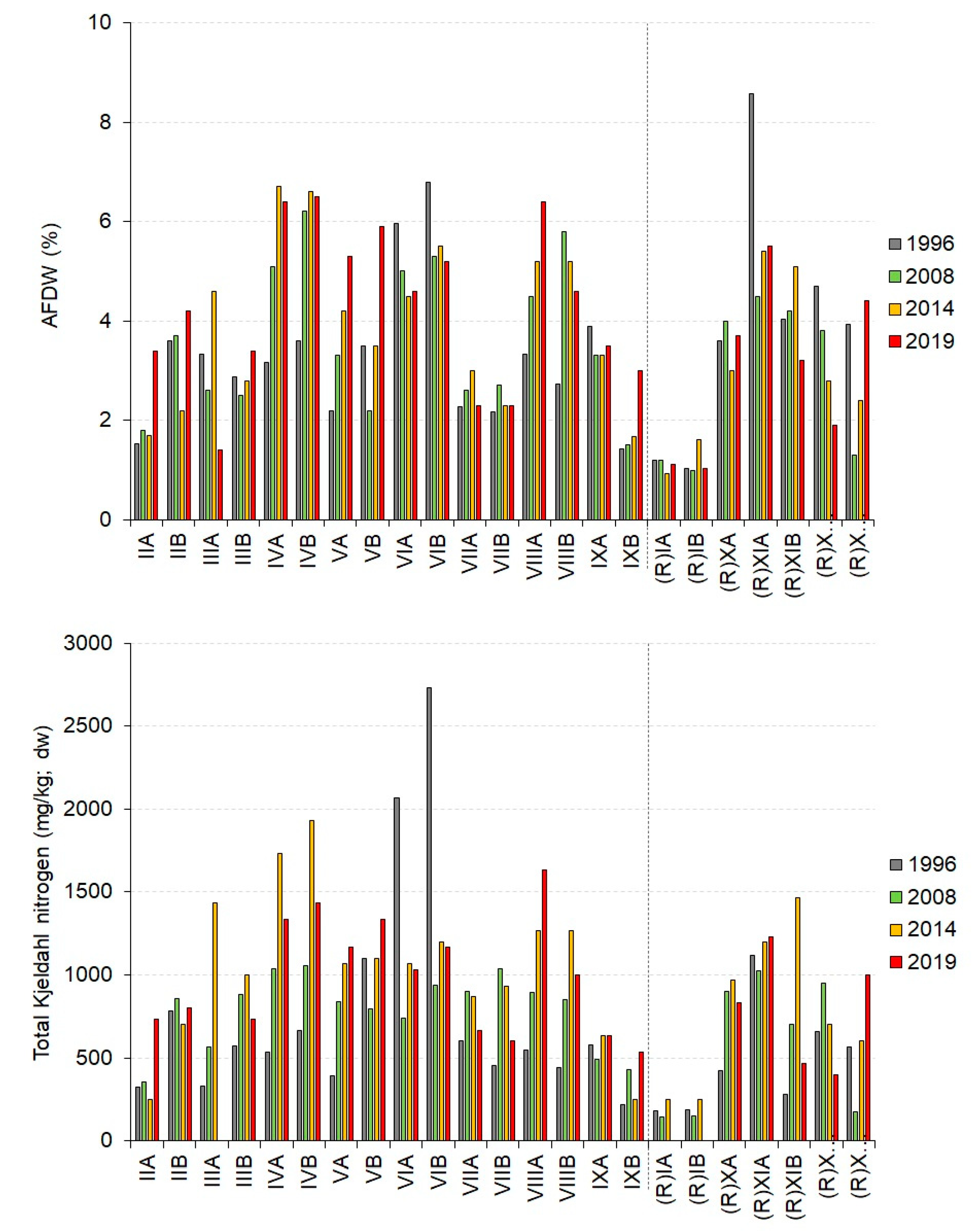
3.2.2. Organic Matter and Nitrogen

Organic content of the sediments (as AFDW) was also relatively stable across time at most sites (Figure 3). There were increases at Application Sites IVA, IVB, VA, and VIIIA, and decreases at Application Site VIA and Reference Site XIIA. These changes often reflected changes in mud content. There was no pattern of change that would suggest an effect of biosolids application. Rather, the increases in mud at some sites is likely to reflect the generally increasing muddiness of Waimea Inlet over time [45].
Concentrations of TN increased at Sites IVA, VA, VB, VIIIA, and IXA (application) and Sites (R)XIA and (R)XIIB over the same three surveys (Figure 3). All other application and reference sites showed no consistent pattern of change over time. Samples from Transect (R)I had the lowest TN concentrations over the years, consistent with its coarser sediment. While there were cumulative increases in sediment TN concentrations over time at some transects, such increases were not consistent among application transects (Figure 3). There were also large differences in TN concentrations between sites (A and B) on the same transect in individual surveys, such as IIIA, IVA, IVB (application), and (R)XIB, or (R)XIIB.

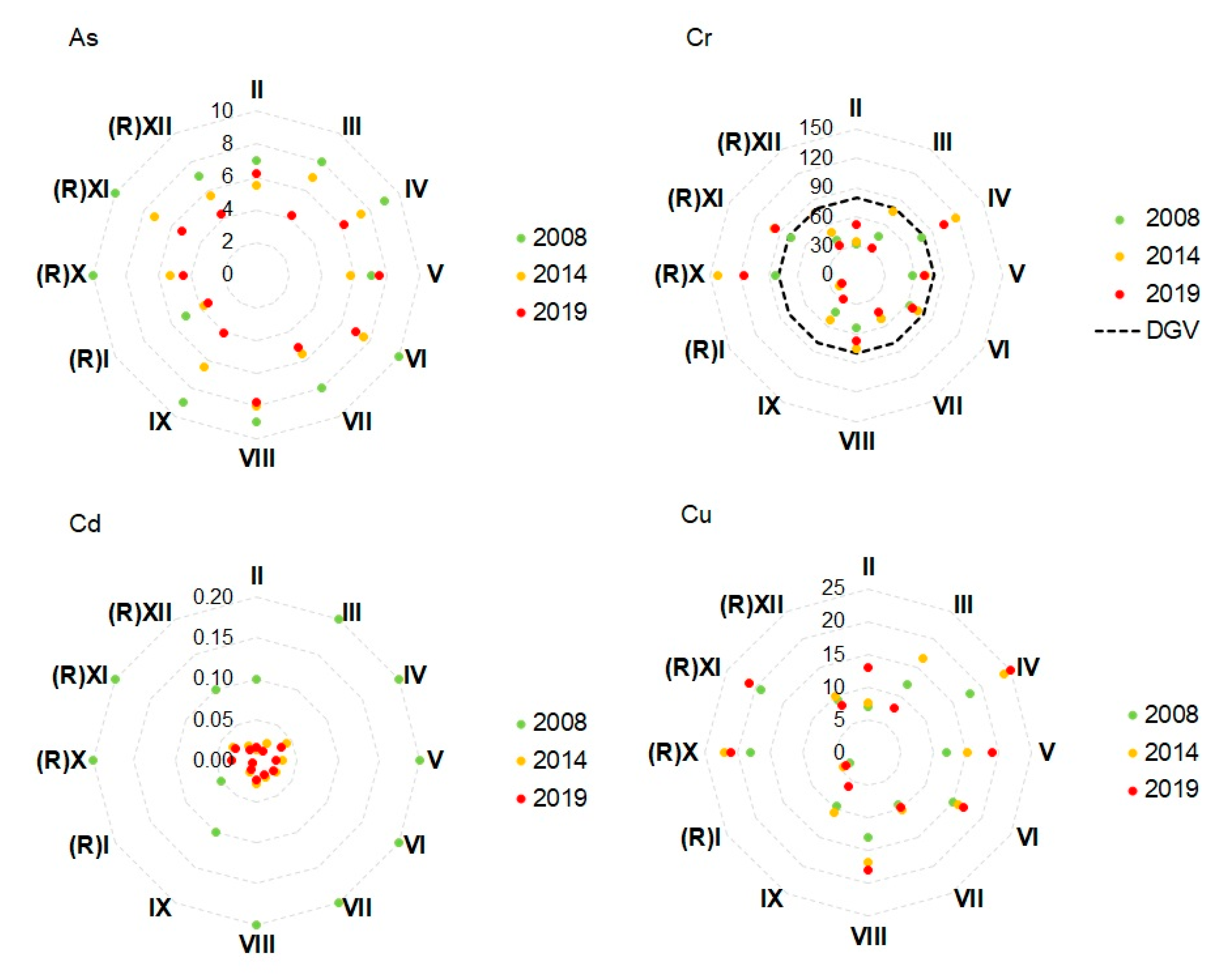
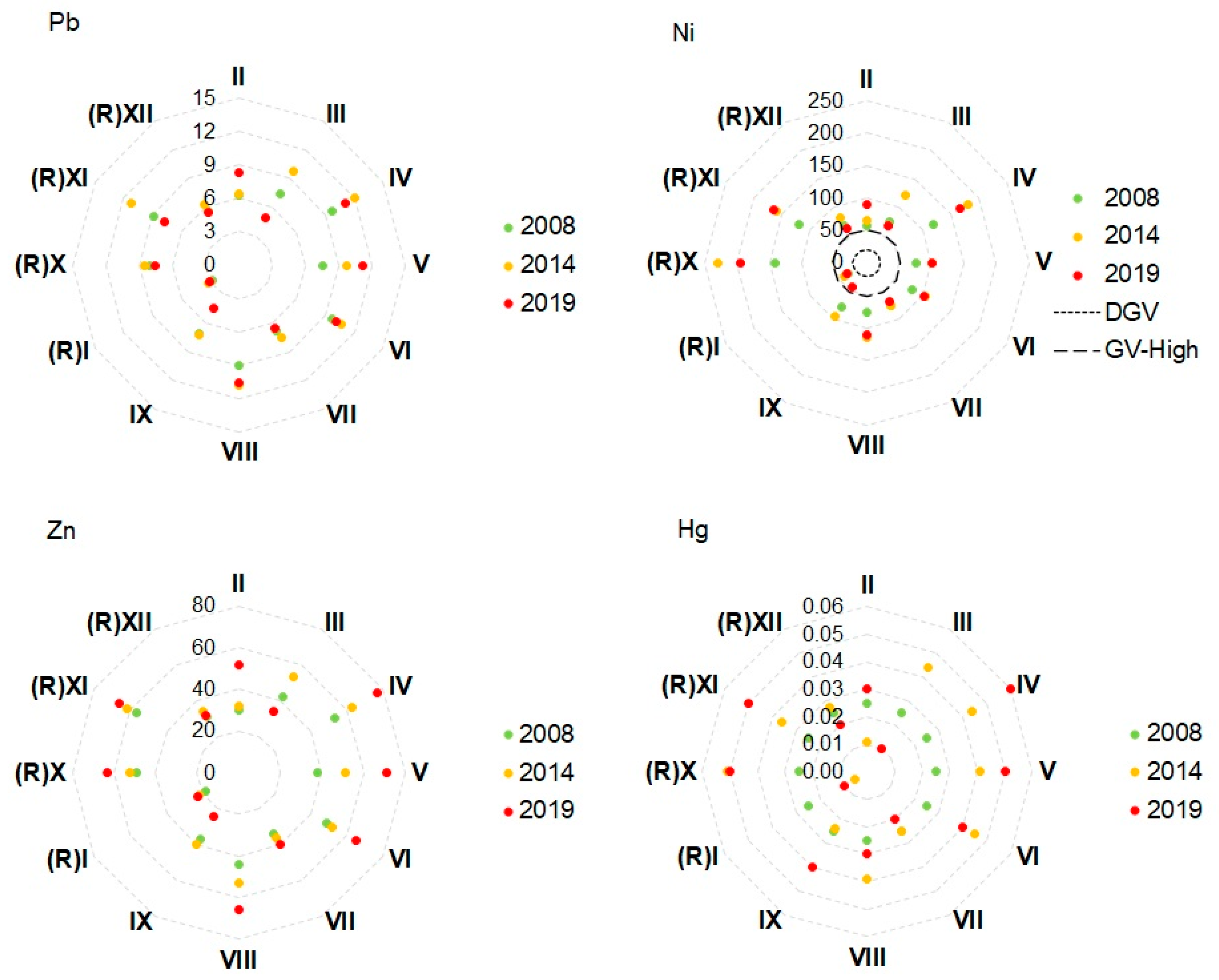
3.2.3. Trace Metals/Arsenic

Concentrations of Cd reduced at all transects over the three consecutive surveys (Figure 4). A reduction in As concentrations was also apparent at most transects, except II and V (application). In contrast, concentrations of Cu, Ni, and Zn increased at some or all transects (Figure 4). However, for all three metals, this pattern was evident at Reference Transects (R)X, (R)XI, and (R)XII and application transects adjacent to biosolids application areas. In fact, concentrations at the reference transects were higher than at several of the application transects; compare, for example, nickel concentrations at Reference Transects (R)X and (R)XI with those at Application Area Transects V and IX. Differences in concentrations of Cr, Pb, and Hg between stations did not show any temporal trends or spatial patterns (differences among application and reference transects) that might suggest that the application of biosolids was causing an accumulation of these metals in coastal sediments over time. Concentrations of As and trace metals at Transect (R)I were consistently low relative to the other transects. Concentrations of As and trace metals were well below the ANZG [40] DGV and GV-High for the protection of aquatic life, except those of Cr and Ni. Both of these exceeded their DGV values and, in the case of Ni, also exceeded the GV-High values.

3.2.4. Faecal Indicator Bacteria

Concentrations of FIB in shellfish were generally higher in the 2014 survey than in the 2008 and 2019 surveys (Table 2). In the 2014 survey, bacterial concentrations at four application and three reference transects exceeded the standard for shellfish-growing areas in the “Approved” status (230 E. coli/100 g) [41]; note that the study area is not used for commercial or recreational shellfish gathering, and this standard was only considered here as a guidance. The highest E. coli concentration was found at Transect (R)X, while the lowest was found at Application Transects VI, VII, and IX.

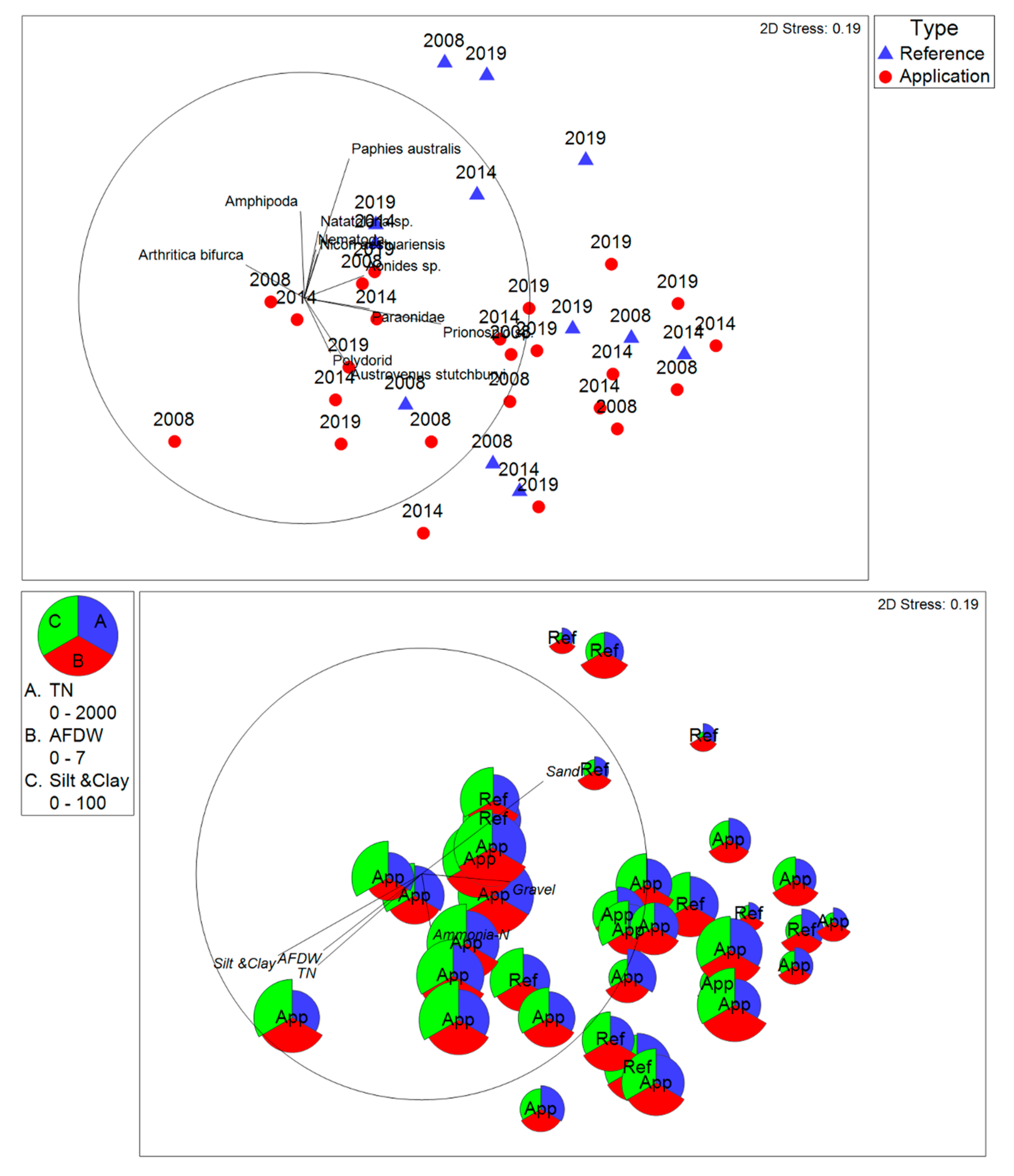
3.2.5. Benthic Infauna Communities

In the 2008 survey, the mean abundance of infauna was higher at the application than at the reference sites; in 2014, the opposite was observed (Table 3: note that there was a large variation in abundance among replicates and transects within treatment groups, as indicated by the relatively high standard deviation (SD)). Mean species richness was higher at the reference sites in the 2008 and 2014 surveys; the opposite was found in the 2019 survey. Mean diversity was higher at the reference sites in the 2008 survey, while in the 2014 and 2019 surveys, mean diversity was higher at the application sites. Species richness, abundance, evenness, and diversity at the application sites were not significantly different from those at the reference sites in any of the survey years (Mann–Whitney test; p > 0.05).
Key infaunal taxa, i.e., those contributing >70% of the total abundance, were similar between the reference and application transects over the three surveys, but their relative abundances varied among years (Table 4). The similarity percentage (SIMPER) analysis of taxa in these groups of transects indicated average dissimilarities of 76% in the 2008 and 2014 surveys and 79% in the 2019 survey. Two taxa indicative of “moderately enriched” conditions (the polychaetes Prionospio sp. and Aonides sp.) [46] made an important contribution to infaunal community composition, particularly in the 2014 and 2019 surveys. Heteromastus filiformis, a polychaete that can also be indicative of “enriched conditions” (AMBI database v6.0, October 2021), was abundant at the application transects, but also found at the reference transects. The bivalve Paphies australis was very abundant at the reference transects, but not at the application ones. Cockles (A. stutchburyi) were equally abundant at the reference and application transects in the 1996 (1.03 and 0.90), 2008 (1.89 and 1.74), and 2014 (2.66 and 2.06) surveys, but not abundant at any transects in the 2019 survey.
Mean abundances of the 10 most-abundant taxa did not differ significantly between the application and reference transects in any of the survey years (Mann–Whitney test, p > 0.01; Table 5). Anthozoa, Nemertea, and Nematoda were the most-abundant taxa in the 2014 and 2019 surveys. In the 1996 survey (pre-disposal), anthozoans were observed at Sites XIIA, XIIB (reference), and IXB (application).
There was no clear distinction between infauna communities at the reference and application transects in any of the survey years, as shown by a non-metric MDS plot of the similarity matrix of the communities (Figure 5). The 2D stress (0.19) was not considered high [43], indicating that the plot provides a reasonable two-dimensional representation of the data. Overlying species (Pearson) correlation vectors on the infaunal nMDS plot (Figure 5) indicates the association of several infaunal taxa, including P. australis, with sandier reference sites in the upper part of the plot and taxa associated with muddier sediments in the centre-right. Overlying physico-chemical environmental variables as bubble plots and (Pearson) correlation vectors on the infaunal nMDS (Figure 5) indicates that sediment composition, organic matter, and TN all show similar correlations with the positions of the samples in the nMDS plot. This similarity is likely to reflect correlation among the environmental variables (higher concentrations of organic matter and TN in finer sediments). There is no indication of any separation of reference and application samples in the direction of these vectors.

3.3. Relationship between Biosolids Application and Nitrogen Concentrations: 2018–2019

The total volumes of biosolids applied to individual forestry blocks during the period November 2018–October 2019 are represented in Figure 6. The highest volume applied was in Block 3.08, in the mid-western part of the Island. Substantial volumes were also applied in blocks near Application Transect IV, followed by lesser volumes at areas near Application Transects V, VI, and IX. No biosolids were applied near Transects (R)XI and (R)XII.
To understand if there was any association between the volume of biosolids applied and the TN concentrations in the sediment, the TN results obtained in the November 2019 survey are plotted as a function of the distance between the transect and the nearest forestry block where biosolids had been applied in the previous year. The results indicated no relationship between these two variables (R2 = 5.3%; F(1,18) = 1.01, p = 0.328), with sites further away from forestry blocks receiving a high volume of biosolids (e.g., (R)XIIB, VIIIA, and (R)XIA) having relatively high TN concentrations in sediment samples (≥1000 mg/kg) (Figure S2).

4. Discussion

Forest fertilisation with biosolids enhances soil fertility and water-holding capacity and decreases erosion and pH buffering, which can increase tree growth, including in soils affected by wildfires [2,3]. Despite these benefits and the large extent of forest lands in many parts of the world, only a small percentage of biosolids generated annually are applied to forest land (2% in NZ) [47]. The protection of ecological integrity is paramount in any biosolids application programme and includes protecting intertidal habitats adjacent to forest lands. The present study evaluated the long-term effects of biosolids applied to forestry plantations on the adjacent intertidal habitats of an estuarine island in NZ (Rabbit Island). The study focused on the intertidal area where groundwater seeps into Waimea Inlet. Overall, no adverse effects were found from the biosolids applications on the enrichment or contaminant status of intertidal habitats or the sediment-living fauna identified.
Changes in shore topography and in the characteristics of the main biological habitats were observed at some coastal sites over the survey years. These changes reflect a progressive trend of erosion of the high shore soil in the study area [48]. Based on the field observations, these changes are likely associated with natural coastal dynamics, potential climate change effects (e.g., sea level rise, extreme weather events), and/or logging activities occurring on Rabbit Island rather than factors related to biosolids applications. Changes in sediment composition were observed over successive surveys at some transects, but statistical analyses of the sediment composition between the application and reference transects indicated that the changes were not related to biosolids application.
No symptoms of enrichment (e.g., excessive algal growth, sediment anoxia, hydrogen sulphide odours, etc.) were observed at most sites surveyed. However, evidence of enrichment in the form of relatively high macroalgal cover and/or potential anoxia in sediment profiles was found at a few sites near biosolids application areas, and high macroalgal cover was found at both the application and reference sites over the survey years. Blooms of macroalgae were found in localised areas throughout Waimea Inlet, particularly those with low sediment oxygenation and in muddy, sulphide-rich sediments, including areas away from the Island [28]. Macroalgae can grow rapidly on Rabbit Island’s shores (and elsewhere in the Inlet), particularly during the early and late summer peak growing periods [22]. Opportunistic taxa (e.g., Ulva sp. and A. chilense) can reach problem densities in estuaries under enriched conditions. In 2004, increased accumulations of macroalgae were found in the upper drainage channel at Transect VI (application), which reduced with improved tidal flushing following the re-opening of the channel at the western end of the Island [31]. Stevens et al. [28] reported an increase in macroalgal cover in 2020 relative to 2014 (expressed as ecological quality rating (EQR); change from EQR = 0.55 or “Moderate” in 2014 to EQR = 0.73 or “Good” in 2020) in parts of the inner estuary characterised by poor sediment quality, low oxygenation, high organic matter and sulphide-rich sediments, and a decrease in estuarine areas around Rough Island (Figure 6).
The results of this study also did not show consistent differences in sediment TN concentration between the application and reference sites over the survey years. Furthermore, we found progressive increases in sediment TN concentrations at sites adjacent to areas that have not received biosolids. Concentrations of TN among estuaries in NZ range from 250–3700 mg/kg (median 250 mg/kg, 75th percentile 747 mg/kg) [49]. The maximum TN concentrations measured in the 2014 (1900 mg/kg) and 2019 (1600 mg/kg) surveys were relatively high compared with other estuaries. A suite of indicators for the condition of estuaries has been developed in NZ, including interim indicators for TN [50]. The indicators place estuarine sediments into bands associated with different levels of stress on sensitive infauna. Concentrations of TN from the 2008, 2041, and 2019 surveys were within bands indicating minor (250–1000 mg/kg) or moderate (1000–2000 mg/kg) stress. Changes in TN tend to reflect changes in sediment composition over time. However, there was no pattern of change that would suggest an effect of biosolids application. Rather, the increases in mud and organic matter at some sites [28] is likely to reflect the generally increasing muddiness of Waimea Inlet over time [51]. This increase is muddiness has been attributed to the development of orchard land in the catchment [28].
Changes in the concentrations of As and some trace metals in sediments over time did not show patterns that might suggest that the application of biosolids was causing an accumulation of any of these potential contaminants. For example, concentrations of Cu, Ni and Zn increased at the reference transects in addition to some application transects. Concentrations of most metals were lower than the respective ANZG [40] guidelines for the protection of aquatic life, the notable exceptions being Cr and Ni. These latter metals occur naturally at relatively high concentrations in coastal sediments in the Nelson region and derive from soils in the catchment [52]. Concentrations of Cr and Ni were elevated to a greater extent at Transects IV (application), (R)X, and (R)XI. These three transects lie close to the outflow of the Waimea River and likely receive the highest inputs of sediment and associated metals from the catchment. Cu and Zn are also ubiquitous contaminants around sites of human activity, entering the aquatic environment via stormwater runoff and frequently accumulating in sediments over time [53].
The interpretation of changes in concentrations of Cd over consecutive surveys is problematic because the values in 2014 and 2019 were consistently much lower than in 2008 and more consistent with other surveys of concentrations in sediments in Waimea Inlet. For example, Cd concentrations in sediments at sites around and downstream of the Bell Island WWTP discharge in the eastern part of Waimea Inlet, sampled in 2016, were in the range of <0.01–0.03 mg/kg [54] and similar to those measured at the study transects in 2014 and 2019. The 2014 and 2019 results suggest that concentrations around the Island are similar to those in other parts of Waimea Inlet and that there is no evidence of an effect from the biosolids application on Cd concentrations.
Concentrations of FIB in shellfish were considerably lower in the 2019 survey than in the previous two surveys. Concentrations of E. coli were below the standard for shellfish-growing areas in the “Approved” status (230 E. coli/100 g) [41]. It is not clear if this represents a general improvement in the microbiological quality of the shellfish at the study sites, because bacterial concentrations can vary widely between sites and even within a single day [55]. However, as per other types of contaminants, the bacterial results did not indicate an effect of the biosolids application on bacterial levels in the shellfish.
The infaunal surveys also provided no evidence of any adverse effects of the biosolids programme on the Island’s infaunal communities. Opportunistic polychaete worms indicative of moderately enriched sediments, such as H. filiformis and Prionospio sp., were recorded at both the reference and application transects. These taxa also occur at other locations within the Inlet, in similar abundances to those in the present study [51]. The mean taxa richness and abundance of infauna communities in the Moturoa/Rabbit Island surveys was also within the range of those occurring in other Waimea Inlet locations and in estuaries throughout NZ [49,51], despite the local variability between the sites surveyed (some in embayments, others in headlands). The presence of polychaete taxa indicative of moderate enrichment at both the application and reference transects and the general similarity of infauna communities at both the reference and potential impact transects were not consistent with an effect of the application of biosolids to land on Moturoa/Rabbit Island.
The higher abundance of P. australis at the reference transects relative to the application transects was consistent with an effect of application. However, Davidson and Moffat [22] found that P. australis has limited tolerance to dilute seawater and fine sediments, and Robertson et al. [51] also found P. australis to be relatively intolerant to mud. Therefore, this result could have been due to the sediment grain size distributions at these transects because the reference sites had lower percentages of silt and clay. Increasing muddiness and eutrophication of estuaries is occurring throughout NZ [49,56] and worldwide [57], largely in direct (e.g., catchment land use change) or indirect (e.g., climate change) responses to human activities.

5. Conclusions and Future Perspectives

Biosolids use in forests and plantations is one of the most-cost-effective and -environmentally safe ways of recycling biosolids. With appropriate biosolids application regimes and the continuing development of wastewater treatment to produce good-quality biosolids, this practice has proven to be environmentally safe. This study found no long-term adverse effects of biosolids application on the adjacent intertidal habitats of Moturoa/Rabbit Island, providing robust evidence that the biosolids application regime is adequate to protect the ecology of nearby marine intertidal habitats in the study area. Although field observations revealed changes in habitat characteristics at a few transects, these changes appeared to be largely attributable to normal variation or factors unrelated to the biosolids applications. No ecological symptoms of biosolid-related over-enrichment were observed, and no evidence was found that biosolids applications resulted in elevated trace metal or arsenic concentrations in the sediments, nor did concentrations of FIB in shellfish appear to be elevated due to the biosolids applications.
Sediment infauna community analyses indicated slight to moderate benthic enrichment at some reference and application monitoring sites, and concentrations of TN were often relatively high compared to other estuaries. Although no conclusion could be drawn regarding the cause, this is likely to reflect a general increase in the muddiness of the Inlet over time, as identified by State of the Environment monitoring and contributions of nitrogen and other contaminants from urban, agricultural, and pastural land use in the catchment.
The indicators of enrichment status found in the surveys may reflect interannual growth patterns of macroalgae and a general trend of nutrient enrichment in Waimea Inlet. However, the enrichment status of some application areas and reference sites may deteriorate in the future due to reasons independent of biosolids application.
The results of this long-term (24 years) monitoring study suggested that processed biosolids can be applied to plantation forests, and potentially other land uses, in coastal areas without necessarily causing adverse effects on adjacent intertidal habitats. This enables sustainable wastewater treatment and recycling of nutrients and organic matter in soils at a relatively low cost and minimal risk to public health [58]. In a global context of rising concern over climate change, environmental pollution, and resource scarcity, there is a compelling need to use biosolids in forest fertilisation/reforestation to facilitate biomass production, soil development, sequestration of atmospheric carbon, and the reduction of greenhouse gas emissions [59]. The generality of this conclusion will depend on local circumstances, including the type of soil and the risk of cumulative effects from other sources of contaminants, and assumes that the rates of application of biosolids are matched to the assimilative capacity of the tree crop. It is also likely that sea level rise, affecting tree growth, the depths of water tables, the frequency and intensity of rainfall, the rates of infiltration, and other factors, will progressively alter the ability of coastal habitats to absorb additional loads of nutrients and other components of biosolids. Future studies could apply sustainability analysis tools (e.g., life cycle assessment, cost–benefit analysis) to better quantify these effects and inform decisions on appropriate application practices while contributing to ecosystem resilience and sustainability [60]. These tools have been successfully applied to study human toxicity effects from the consumption of agricultural products grown in biosolid-amended soils [61] and to benchmark the environmental impact of wastewater treatment facilities while optimizing resource utilization [62].
A limitation of the present study was that it did not address potential ecological effects associated with emerging organic contaminants (e.g., pharmaceuticals, personal care products, pesticides, plasticisers), which can have detrimental effects on aquatic fauna and flora and coastal communities that depend on these natural resources [63]. Generally, local authorities do not include emerging organic contaminants in routine discharge-consent-monitoring programmes. Further research is needed to characterise the fate and transport of these contaminants in coastal forestry plantations.

Supplementary Materials

The following Supporting Information can be downloaded at: https://www.mdpi.com/article/10.3390/su151612279/s1, Figure S1: Total daily volume of biosolids applied to forestry blocks on Moturoa/Rabbit Island after the baseline survey, 1997–2019; Figure S2: Scatterplot of concentrations of total nitrogen in sediment samples as a function of distance from the nearest Moturoa/Rabbit Island biosolids application area in the 2019 survey; Table S1: Grain size, nutrient, chemical, and microbiological testing methods used in the study.

Author Contributions

Conceptualization, C.J.A.C., D.M., P.G. and N.C.; methodology, C.J.A.C. and D.M.; investigation, data curation, writing—original draft preparation, review and editing, C.J.A.C., A.B., F.M., L.F., D.M., P.G. and N.C. All authors have read and agreed to the published version of the manuscript.

Funding

This research was funded by the Nelson Regional Sewerage Business Unit through the project “Estuarine impacts of the land disposal of biosolids on Rabbit Island”.

Data Availability Statement

The data reported in this article are available upon request.

Acknowledgments

We thank the numerous Cawthron staff who assisted with the fieldwork, sample processing, and laboratory analyses over the years of the monitoring programme. Thanks also to Sam Nuske and Melanie McCuish (PF Olsen Ltd.) for providing information on forestry blocks and logistical support during the fieldwork, Malcolm Furness (NMWaste) for logistical support, and Hill Laboratories Ltd.

Conflicts of Interest

The authors declare no conflict of interest.

References

  1. Gianico, A.; Braguglia, C.M.; Gallipoli, A.; Montecchio, D.; Mininni, G. Land application of biosolids in Europe: Possibilities, con-straints, and future perspectives. Water 2021, 13, 102. [Google Scholar] [CrossRef]
  2. Magesan, G.N.; Wang, H. Application of municipal and industrial residuals in New Zealand forests: An overview. Aus. J. Soil Res. 2003, 41, 557–569. [Google Scholar] [CrossRef]
  3. Bai, J.; Sun, X.; Xu, C.; Ma, X.; Huang, Y.; Fan, Z.; Cao, X. Effects of sewage sludge application on plant growth and soil characteristics at a Pinus sylvestris var. mongolica plantation in Horqin sandy land. Forests 2022, 13, 984. [Google Scholar]
  4. National Resource Council. Biosolids Applied to Land: Advancing Standards and Practices; The National Academies Press: Washington, DC, USA, 2002.
  5. Gerba, C.P.; Pepper, I.L. Wastewater treatment and biosolids reuse. In Environmental Microbiology, 2nd ed.; Academic Press Inc.: Cambridge, MA, USA, 2009; pp. 503–530. [Google Scholar]
  6. Atalay, A.; Bronick, C.; Pao, S.; Mersie, W.; Kalantari, A.; Mcnamee, C.; Whitehead, B. Nutrient and microbial dynamics in biosolids amended soils following rainfall simulation. Soil Sed. Contam. Int. J. 2007, 16, 209–219. [Google Scholar] [CrossRef]
  7. McLaren, R.G.; Black, A.; Clucas, L.M. Changes in Cu, Ni, and Zn availability following simulated conversion of biosolids-amended forest soils back to agricultural use. Aus. J. Soil. Res. 2010, 48, 286–293. [Google Scholar] [CrossRef]
  8. Xue, J.; Kimberley, M.O.; Ross, C.; Gielen, G.; Tremblay, L.A.; Champeau, O.; Horswell, J.; Wang, H. Ecological impacts of long-term application of biosolids to a radiata pine plantation. Sci. Total Environ. 2015, 530–531, 233–240. [Google Scholar] [CrossRef] [PubMed]
  9. Wang, M.; Xue, J.; Horswell, J.; Kimberley, M.O.; Huang, Z. Long-term biosolids application alters the composition of soil microbial groups and nutrient status in a pine plantation. Biol. Fert. Soils 2017, 53, 799–809. [Google Scholar] [CrossRef]
  10. NZWWA. Guidelines for the Safe Application of Biosolids to Land in New Zealand. Report to the New Zealand Water and Wastes Association and Ministry for the Environment. 2003. Available online: https://www.waterA/NZ.org.A/NZ/Folder?Action=View%20File&Folder_id=101&File=biosolids_guidelines.pdf (accessed on 5 May 2023).
  11. Magesan, G.N.; Wang, H.; Clinton, P. Best Management Practices for Applying Biosolids to Forest Plantations in New Zealand. SCION Report 45869. 2010. Available online: https://envirolink.govt.A/NZ/assets/Envirolink/742-TSDC53-Best-management-practices-for-applying-biosolids-to-forests.pdf (accessed on 5 May 2023).
  12. Ippolito, J.A.; Ducey, T.F.; Diaz, K.; Barbarik, K.A. Long-term biosolids land application influences soil health. Sci. Total Environ. 2021, 791, 148344. [Google Scholar] [CrossRef] [PubMed]
  13. Grey, M.; Henry, C. Phosphorus and nitrogen runoff from a forested watershed fertilized with biosolids. J. Environ. Qual. 2002, 31, 926–936. [Google Scholar] [CrossRef]
  14. Abreu-Junior, C.H.; de Oliveira, M.G.; Cardoso, P.H.S.; Mandu, T.d.S.; Florentino, A.L.; Oliveira, F.C.; dos Reis, J.V.; Alvares, C.H.; Stape, J.L.; Nogueira, T.A.R.; et al. Sewage sludge application in Eucalyptus urograndis plantation: Availability of phosphorus in soil and wood production. Front. Environ. Sci. 2020, 8, 116. [Google Scholar] [CrossRef]
  15. Da Silva, P.H.M.; Poggiani, F.; Laclau, J.P. Applying sewage sludge to Eucalyptus grandis plantations: Effects on biomass production and nutrient cycling through litterfall. Appl. Environ. Soil Sci. 2011, 2011, 710614. [Google Scholar] [CrossRef] [Green Version]
  16. Gutiérrez-Ginés, M.; Robinson, B.H.; Esperschuetz, J.; Madejón, E.; Horswell, J.; McLenaghen, R. Potential use of biosolids to reforest degraded areas with New Zealand native vegetation. J. Environ. Qual. 2017, 46, 906–914. [Google Scholar] [CrossRef] [PubMed] [Green Version]
  17. Nelson Regional Sewerage Business Unit. Wastewater Asset Management Plan. 2017. Available online: http://www.nrsbu.govt.nz/assets/NRSBU/Plans-and-reports/amp/Nelson-Regional-Sewerage-Business-Unit-Asset-Management-Plan-2017.pdf (accessed on 5 May 2023).
  18. Fryer, B. Model Based Study of Autothermal Thermophilic Aerobic Digestion (ATAD) Processes. Masters’ Thesis, Massey University, Palmerston North, New Zealand, 2000. [Google Scholar]
  19. Ballard, R. Use of fertilisers at establishment of exotic forest plantations in New Zealand. N. Z. J. For. Sci. 1978, 8, 70–104. [Google Scholar]
  20. Wilks, P.; Haddon, S. Tasman District Council Forest Management Plan for the period 2014/2019. PF Olsen Report FSCGS04. 2014. Available online: https://pfolsen.blob.core.windows.net/productionmedia/2198/tdc_mp14.pdf (accessed on 5 May 2023).
  21. Tonkin and Taylor. Moturoa/Rabbit Island Biosolids Reconsenting. Assessment of Effects on the Environment. Prepared for Nelson Regional Sewerage Business Unit by Tonkin & Taylor Ltd. 2020. Available online: https://www.tasman.govt.nz/document/serve/01A%20RM200638%20NRSBU%20-%20Application%20AEE%20-%20AEE%20Apps%20A%20to%20C.pdf?DocID=31414 (accessed on 5 May 2023).
  22. Davidson, R.J.; Moffat, C.R. A Report on the Ecology of Waimea Inlet, Nelson; Department of Conservation, Nelson/Marlborough Conservancy Occasional Publication: Nelson, New Zealand, 1990; No. 1. [Google Scholar]
  23. Robertson, B.M.; Gillespie, P.A.; Asher, R.A.; Frisk, S.; Keeley, N.B.; Hopkins, G.A.; Thompson, S.J.; Tuckey, B.J. Estuarine Environmental Assessment and Monitoring: A National Protocol. Part A. Development, Part B. Appendices, Part C. Application. 2002. Available online: https://docs.niwa.co.nz/library/public/EMP_part_c.pdf (accessed on 7 March 2023).
  24. Stevens, L.M.; Robertson, B.M. Nelson Region Estuaries: Vulnerability Assessment and Monitoring Recommendations; Wriggle Coastal Management for Nelson City Council: Nelson, New Zealand, 2017; 36p. Available online: https://www.nelson.govt.nz/assets/Environment/Downloads/Environmental-monitoring/estuarine-health/NCC-regional-estuarine-monitoring-and-reporting-WRIGGLE-vulnerability-assessment-2017.pdf (accessed on 7 August 2023).
  25. Hume, T.; Gerbeaux, P.; Hart, D.; Kettles, H.; Neale, D. A Classification of New Zealand’s Coastal Ecosystems. NIWA Client Report No. HAM2016-062 prepared for the Ministry for the Environment. 2016. Available online: https://ir.canterbury.ac.A/NZ/bitstream/handle/10092/15225/a-classification-of-A/NZ-coastal-hydrosystems.pdf?sequence=2 (accessed on 5 May 2023).
  26. Heath, R.A. Broad classification of New Zealand inlets with emphasis on residence times. N. Z. J. Mar. Freshw. Res. 1976, 10, 429–444. [Google Scholar] [CrossRef]
  27. Whitehead, A.L.; Booker, D.J. NZ River Maps: An Interactive Online Tool for Mapping Predicted Freshwater Variables across New Zealand. NIWA, Christchurch. 2020. Available online: https://shiny.niwa.co.nz/nzrivermaps/ (accessed on 5 May 2023).
  28. Stevens, L.M.; Scott-Simmonds, T.; Forrest, B.M. Broad Scale Intertidal Monitoring of Waimea Inlet; Salt Ecology Report 052; Tasman District and Nelson City Councils: Richmond, New Zealand, 2020; 50p.
  29. Tasman District Council. Tasman Resource Management Plan (TRMP). 2018. Available online: https://www.tasman.govt.A/NZ/my-council/key-documents/tasman-resource-management-plan/ (accessed on 5 May 2023).
  30. Wilks, P.; Wang, H. The Rabbit Island Biosolids Project. A/NZ J. For. 2009, 54, 33–36. [Google Scholar]
  31. Gillespie, P.; Asher, R. Estuarine Impacts of the Land Disposal of Sewage Sludge on Rabbit Island: 2003 Monitoring Survey; Cawthron Report No. 862; Nelson Regional Sewerage Business Unit: Nelson, New Zealand, 2004.
  32. Nelson City Council. State of the Environment Report. 2020. Available online: http://www.nelson.govt.A/NZ/council/plans-strategies-policies/strategies-plans-policies-reports-and-studies-a-z/state-of-the-environment-reports/ (accessed on 5 May 2023).
  33. Gillespie, P. Benthic and Planktonic Microalgae in Tasman Bay: Biomass Distribution, and Implications for Shellfish Growth; Motueka Integrated Catchment Management (Motueka ICM) Programme Report Series; Cawthron Report No. 835; Cawthron Institute: Nelson, New Zealand, 2003. [Google Scholar]
  34. Gillespie, P.A.; Maxwell, P.D.; Rhodes, L.L. Microphytobenthic communities of subtidal locations in New Zealand: Taxonomy, biomass, production, and food-web implications. N. Z. J. Mar. Freshw. Res. 2000, 34, 41–53. [Google Scholar] [CrossRef]
  35. FAO. Standard Operating Procedure for Soil Total Nitrogen—Dumas Dry Combustion Method. 2021. Available online: https://www.fao.org/3/cb3646en/cb3646en.pdf (accessed on 5 August 2023).
  36. D422-63; Standard Test Method for Particle-Size Analysis of Soils. ASTM: West Conshohocken, PA, USA, 2007. Available online: https://www.astm.org/d0422-63r07.html (accessed on 5 August 2023).
  37. APHA. 3125 Metals by Inductively Coupled Plasma-Mass Spectrometry. In Standard Methods for the Examination of Water and Wastewater, 24th ed.; Lipps, W.C., Baxter, T.E., Braun-Howland, E., Eds.; APHA: Washington, DC, USA, 2022; Available online: https://www.standardmethods.org/doi/10.2105/smww.2882.048 (accessed on 5 August 2023).
  38. APHA. Compendium of Methods for the Microbiological Examination of Foods, 5th ed.; Salfinger, Y., Tortorello, M.L., Eds.; APHA: Washington, DC, USA, 2015; Chapter 9.8; Available online: https://ajph.aphapublications.org/doi/abs/10.2105/MBEF.0222 (accessed on 5 October 2021).
  39. APHA. 9230 Fecal Enterococcus/Streptococcus Groups. In Standard Methods for the Examination of Water and Wastewater, 23rd ed.; APHA: Washington, DC, USA, 2018. [Google Scholar] [CrossRef]
  40. ANZG. Toxicant default guideline values for sediment quality. In Australian and New Zealand Guidelines for Fresh and Marine Water Quality; Australian and New Zealand Governments and Australian State and Territory Governments: Canberra ACT, Australia, 2018. Available online: https://www.waterquality.gov.au/anz-guidelines/guideline-values/default/sediment-quality-toxicants (accessed on 5 May 2023).
  41. Ministry for Primary Industries. Animal Products Notice: Regulated Control Scheme—Bivalve Molluscan Shellfish for Human Consumption. 2018. Available online: https://www.mpi.govt.A/NZ/dmsdocument/30282-animal-products-notice-regulated-control-scheme-bivalve-molluscan-shellfish-for-human-consumption-2018 (accessed on 5 May 2023).
  42. Pielou, E.C. Ecological Diversity; John Wiley & Sons: New York, NY, USA, 1975. [Google Scholar]
  43. Sturrock, K.; Rocha, J. A multidimensional scaling stress evaluation table. Field Methods 2000, 12, 49–60. [Google Scholar] [CrossRef]
  44. Clarke, K.R.; Gorley, R.N.; PRIMER v7: User Manual/Tutorial. PRIMER-E: Plymouth. 2015. Available online: http://updates.primer-e.com/primer7/manuals/User_manual_v7a.pdf (accessed on 5 May 2023).
  45. Stevens, L.M.; Robertson, B.M. Waimea Inlet 2010: Vulnerability Assessment and Monitoring Recommendations; Wriggle Coastal Management for Tasman District Council: Richmond, New Zealand, 2010; 58p.
  46. Keeley, N.B.; Macleod, C.K.; Forrest, B.M. Combining best professional judgement and quantile regression splines to improve characterisation of macrofaunal responses to enrichment. Ecol. Ind. 2012, 12, 154–166. [Google Scholar] [CrossRef]
  47. Tinholt, R. The Value of Biosolids in New Zealand—An Industry Assessment. Paper presented at the Water New Zealand Conference & Expo. 2019. Available online: https://www.waternz.org.nz/Attachment?Action=Download&Attachment_id=4029 (accessed on 5 May 2023).
  48. Tasman District Council. Moturoa/Rabbit Island Reserve Management Plan. Council Report RCN16-09-08. 2016. Available online: https://www.google.com/url?sa=i&rct=j&q=&esrc=s&source=web&cd=&cad=rja&uact=8&ved=0CAIQw7AJahcKEwiord-M1u__AhUAAAAAHQAAAAAQAg&url=https%3A%2F%2Fwww.tasman.govt.nz%2Fdocument%2Fserve%2FMoturoa-Rabbit%2520Island%2520Reserve%2520Management%2520Plan%25202016.pdf%3FDocID%3D29383&psig=AOvVaw0yBchehP7inUEhaGXEwRUs&ust=1688374886043243&opi=89978449 (accessed on 7 August 2023).
  49. Berthelsen, A.; Atalah, J.; Clark, D.; Goodwin, E.; Sinner, J.; Patterson, M. New Zealand estuary benthic health indicators summarised nationally and by estuary type. N. Z. J. Mar. Freshw. Res. 2019, 54, 24–44. [Google Scholar] [CrossRef]
  50. Robertson, B.M.; Stevens, L.; Robertson, B.; Zeldis, J.; Green, M.; Madarasz-Smith, A.; Plew, D.; Storey, R.; Oliver, M. A/NZ Estuary Trophic Index Screening Tool 2. Determining Monitoring Indicators and Assessing Estuary Trophic State; Prepared for Envirolink Tools Project: Estuarine Trophic Index, MBIE/NIWA Contract No: C01X1420; Wriggle Limited: Nelson, New Zealand, 2016. [Google Scholar]
  51. Robertson, B.; Robertson, B. Waimea Inlet Fine Scale Monitoring 2013/14. Wriggle Coastal Management Report Prepared for Tasman District Council. 2014. Available online: https://waimeainlet.wordpress.com/resource-documents/ (accessed on 5 May 2023).
  52. Forrest, B.M.; Gillespie, P.A.; Cornelisen, C.D.; Rogers, K.M. Multiple indicators reveal river plume influence on sediments and benthos in a New Zealand coastal embayment. N. Z. J. Mar. Freshw. Res. 2007, 41, 13–24. [Google Scholar] [CrossRef]
  53. Williamson, R.B.; Morrisey, D.J. Stormwater contamination of urban estuaries. 1. Predicting the build-up of heavy metals in sediments. Estuaries 2000, 23, 56–66. [Google Scholar] [CrossRef]
  54. Morrisey, D.; Webb, S. Coastal Effects of the Nelson (Bell Island) Regional Sewerage Discharge: Benthic Monitoring Survey 2016; Cawthron Report No. 2979; Nelson Regional Sewerage Business Unit: Nelson, New Zealand, 2017.
  55. Boehm, A.B. Enterococci concentrations in diverse coastal environments exhibit extreme variability. Environ. Sci. Technol. 2007, 41, 8227–8232. [Google Scholar] [CrossRef] [PubMed] [Green Version]
  56. MacDiarmid, A.; McKenzie, A.; Sturman, J.; Beaumont, J.; Mikaloff-Fletcher, S.; Dunne, J. Assessment of Anthropogenic Threats to New Zealand Marine Habitats; New Zealand Aquatic Environment and Biodiversity Report No 9; New Zealand Ministry of Agriculture and Forestry: Wellington, New Zealand, 2012; Volume 3, 255p.
  57. Lotze, H.K.; Lenihan, H.S.; Bourque, B.J.; Bradbury, R.H.; Cooke, R.G.; Kay, M.C.; Kidwell, S.M.; Kirby, M.X.; Peterson, C.H.; Jackson, J.B.C. Depletion, degradation, and recovery potential of estuaries and coastal seas. Science 2006, 312, 1806–1809. [Google Scholar] [CrossRef] [PubMed]
  58. Wang, H.; Brown, S.L.; Magesan, G.N.; Slade, A.H.; Quintern, M.; Clinton, P.W.; Payn, T.W. Technological options for the management of biosolids. Environ. Sci. Pollut. Res. 2008, 15, 308–317. [Google Scholar] [CrossRef] [PubMed]
  59. UN-HABITAT, Greater Moncton Sewerage Commission. Global Atlas of Excreta, Wastewater Sludge, and Biosolids Management: Moving Forward the Sustainable and Welcome Uses of a Global Resource; LeBlanc, R.J., Matthews, P., Richard, R.P., Eds.; United Nations Human Settlements Programme (UN-HABITAT): Nairobi, Kenya, 2008; Available online: https://unhabitat.org/global-atlas-of-excreta-wastewater-sludge-and-biosolids-management (accessed on 5 May 2023).
  60. Brown, S.; Ippolito, J.A.; Hundal, L.S.; Basta, N.T. Municipal biosolids—A resource for sustainable communities. Curr. Opin. Environ. Sci. Health 2020, 14, 56–62. [Google Scholar] [CrossRef]
  61. Sablayrolles, C.; Gabrielle, B.; Montrejaud-Vignoles, M. Life cycle assessment of biosolids land application and evaluation of the factors impacting human toxicity through plant uptake. J. Ind. Ecol. 2010, 14, 231–241. [Google Scholar] [CrossRef] [Green Version]
  62. Alayna, S.; Dewulf, J.; Duran, M. Comparison of overall resource consumption of biosolids management system processes using exergetic life cycle assessment. Environ. Sci. Technol. 2015, 49, 9996–10006. [Google Scholar] [CrossRef]
  63. Gwenzi, W.; Simbanegavi, T.T.; Marumure, J.; Makuvara, Z. Chapter 13—Ecological health risks of emerging organic contaminants. In Emerging Contaminants in the Terrestrial-Aquatic-Atmosphere Continuum: Occurrence, Health Risks and Mitigation; Gwenzi, W., Ed.; Elsevier: Amsterdam, The Netherlands, 2022; pp. 215–242. [Google Scholar]
Figure 1. Locations of sampling transects on Moturoa/Rabbit Island. Arrows indicate the direction of groundwater flow through the Island.
Sustainability 15 12279 g001
Figure 2. Sediment composition at biosolids application and reference stations in the Moturoa/Rabbit Island shoreline in the three surveys. The labels on the “x” axis indicate the transect IDs. IDs to the left of the dashed line are “application” sites; those to the right are “reference” sites.
Sustainability 15 12279 g002
Figure 3. Concentrations of ash-free dry weight (AFDW) and total nitrogen (TN) in sediment samples collected at the application and reference sites on the Moturoa/Rabbit Island shoreline in three consecutive surveys. “(R)” indicates reference sites. Missing data represent values less than the analytical limits of detection (200 mg/kg for TN). The labels on the “x” axis indicate the transect IDs. IDs to the left of the dashed line are “application” sites; those to the right are “reference” sites.
Sustainability 15 12279 g003
Figure 4. Radar plots of concentrations of arsenic and trace metals in sediment samples collected at the application and reference sites on the Moturoa/Rabbit Island shoreline in three consecutive surveys. The dotted black line and heavy dotted black line denote ANZG [40] DGV and GV-High, respectively, which were exceeded in the samples for Ni and Cr. Other DGV and GV-High guidelines that were not exceeded were: As—20, 70; Cd—1.5, 10; Cu—65, 270; Pb—50, 2020; Zn—200, 410; Hg—0.15, 1.0.
Sustainability 15 12279 g004aSustainability 15 12279 g004b
Figure 5. Results of non-metric multidimensional scaling of the infaunal communities (averaged per transect per year) for the three survey years. In the upper plot, blue and red triangles show the reference and application transects, respectively, and are labelled per survey year. Species (Pearson) correlation vectors indicate the associations of species with samples. In the lower plot, bubbles representing values of environmental variables are overlayed on the same infaunal nMDS to illustrate relationships between infaunal and sediment-related variables. The vectors in this plot represent Pearson correlations of environmental variables with the positions of infaunal samples in the plot. Bray–Curtis similarity; data transformed using the square root. The ranges of values for total nitrogen (TN) are mg/kg, and ash-free dry weight (AFDW) and silt/clay are percent by dry weight.
Sustainability 15 12279 g005
Figure 6. Total volume of biosolids applied to forestry blocks on Moturoa/Rabbit Island during the period November 2018–October 2019. Transects I, X, XI, and XII are references.
Sustainability 15 12279 g006
Table 1. Summary of Moturoa/Rabbit Island shoreline observations made in the 1996, 2008, 2014, and 2019 surveys. Orange shading indicates macroalgal cover >10%.
Transect Number
ApplicationReference
Survey YearSiteIIIIIIVVVIVIIVIIIIXIXXIXII
Approximate transect length (m) 1602624507525246040247060
Average density of crab holes 11996A1152521192151537-5623
B11171524161388-n/s54
Macroalgal % cover B000509060<5<5000<5
Average density of crab holes 12008A213923514354320.23619
B20202317185430.61 61
Macroalgal % cover B00000<51600<59
Average density of crab holes 12014A1267731461076230.2724
B251713214626321n/s190
Macroalgal % cover B00000360130n/s<419
Average density of crab holes 12019A501220920634250530.8
B524847131190.30020.08
Macroalgal % cover B0008087750350333432
1 Average/0.1 m2; sites with high macroalgal cover highlighted in orange. n/s denotes no site, the area being in the channel. (-) denotes not recorded.
Table 2. Concentrations of faecal indicator bacteria in shellfish samples collected at application and reference sites on the Moturoa/Rabbit Island shoreline in three consecutive surveys. ns—no sample collected or insufficient number of shellfish. E. coli results that exceeded the standard for shellfish-growing areas in the “Approved” status (230/100 g) are shaded in orange.
200820142019
TransectEnterococciE. coliEnterococciE. coliEnterococciE. coli
Application
II11050240079040<30
III<2020700330<30<30
IV17020120170nsns
V490330>16,0002200nsns
VI170<20490790nsns
VII20<2023040<30<30
VIII1302046050nsns
IX20<201300170<30<30
Reference
I20807907904092
X14049035003500902100
XI2020270130070<30
XII507005080<30<30
Table 3. Infaunal community indices at the application and reference transects on the Moturoa/Rabbit Island shoreline in the three survey years.
Taxonomic GroupApplication
(II, III, IV, V, VI, VII, VIII, IX)
Reference
(I, X, XI, XII)
MeanSDMeanSD
2008 survey
Species richness7.94.18.174.12
Abundance65.362.846.2542.90
Evenness0.70.10.760.13
Diversity1.30.41.520.38
2014 survey
Species richness12.16.113.335.1
Abundance123.8103.2155.1166.1
Evenness0.70.10.620.14
Diversity1.70.41.570.4
2019 survey
Species richness13.27.210.834.88
Abundance101.97.4107.656.1
Evenness0.70.10.640.11
Diversity1.70.51.480.43
Table 4. Average abundances (number of individuals per core) of infauna taxa on the Moturoa/Rabbit Island shoreline contributing the highest percentages (>70% contribution) to the dissimilarity between the application and reference transects per survey year (SIMPER analysis, square-root-transformed sample data).
SurveyTaxonAverage Abundance (Individuals/m2)
Reference
(I, X, XI, XII)
Application
(II, III, IV, V, VI, VII, VIII, IX)
Av. DissDiss/SD% Contrib% Cum
2008 aPrionospio sp.1.993.039.191.2812.0912.09
Arthritica bifurca0.61.736.320.878.3220.41
Heteromastus filiformis0.962.176.021.27.9328.34
Austrovenus stutchburyi1.891.745.861.037.7136.05
Paphies australis1.310.185.080.566.6942.74
Amphipoda1.150.724.460.865.8748.61
Paraonidae1.250.784.011.015.2853.89
Nicon aestuariensis0.770.93.580.854.7158.6
Hemiplax hirtipes0.70.823.190.954.262.8
Austrohelice crassa00.52.570.593.3866.18
Linucula hartvigiana0.610.642.490.613.2769.45
Cirratulidae0.810.22.150.642.8372.28
2014 bPrionospio sp.3.223.787.011.359.239.23
Aonides sp.3.81.315.520.87.2616.49
Arthritica bifurca1.32.35.020.996.6123.1
Paphies australis1.9804.550.575.9929.09
Austrovenus stutchburyi2.662.064.291.255.6534.73
Amphipoda2.251.034.140.825.4540.18
Paraonidae1.012.384.030.775.345.48
Heteromastus filiformis0.941.883.370.934.4349.91
Polydorid1.141.063.030.943.9953.9
Amphibola crenata0.540.852.440.783.2157.11
Nereididae (juvenile)0.990.921.941.082.5559.66
Austrominius modestus0.250.721.830.522.4162.07
Oligochaeta0.640.641.650.92.1864.24
Notoacmea sp.0.670.741.640.582.1666.41
Austrohelice crassa0.530.531.610.852.1268.53
Hemiplax hirtipes0.620.871.571.062.0670.59
2019 cPaphies australis3.340.467.380.879.369.36
Prionospio sp.2.432.315.6817.216.56
Amphipoda2.921.595.210.956.623.17
Oligochaeta2.351.84.561.165.7928.95
Polydorid0.142.014.3115.4734.42
Paraonidae0.752.324.20.775.3339.75
Arthritica bifurca1.161.163.570.784.5344.27
Amphibola crenata0.521.233.290.834.1748.45
Aonides sp.0.22.073.290.614.1752.61
Exosphaeroma sp.1.560.33.230.844.156.71
Nicon aestuariensis1.580.452.961.133.7560.46
Heteromastus filiformis0.81.022.340.932.9663.42
Hemiplax hirtipes0.621.42.241.272.8466.26
Nemertea0.581.171.891.22.468.66
Natatolana sp.0.790.061.860.872.3671.02
a Average dissimilarity = 76.00. b Average dissimilarity = 76.01. c Average dissimilarity = 78.86. Av. Diss—average dissimilarity; Diss/SD—dissimilarity/standard deviation; % Contrib—percentage contribution; % Cum—cumulative percentage.
Table 5. Abundance (number of individuals per core) of the 10 most-abundant taxa at the application transects versus the same taxa at the reference transects on the Moturoa/Rabbit Island shoreline in the three survey years.
SurveyTaxonApplication
(II, III, IV, V, VI, VII, VIII, IX)
TaxonReference
(I, X, XI, XII)
MeanSDMeanSD
2008Prionospio sp.23.542.9Prionospio sp.10.621.2
Heteromastus filiformis9.011.2Paphies australis6.413.1
Arthritica bifurca7.512.9Austrovenus stutchburyi5.35.8
Austrovenus stutchburyi5.37.5Paraonidae4.210.5
Linucula hartvigiana3.49.7Heteromastus filiformis3.06.6
Oligochaeta3.39.2Amphipoda2.83.6
Paraonidae2.37.3Cirratulidae2.86.2
Amphipoda1.83.7Linucula hartvigiana1.63.3
Macomona liliana1.75.1Nicon aestuariensis1.52.2
Nicon aestuariensis1.41.6Arthritica bifurca1.12.3
2014Anthozoa26.70.5Anthozoa50.10.0
Nemertea23.91.0Nemertea34.80.8
Nematoda13.10.0Nematoda13.80.0
Sipuncula9.40.3Sipuncula11.90.0
Chiton glaucus9.00.4Chiton glaucus9.80.3
Ischnochiton maorianus7.40.0Ischnochiton maorianus5.00.0
Gastropoda (micro snails)3.60.2Gastropoda (micro snails)3.60.3
Pyramidellidae3.50.0Pyramidellidae3.30.0
Amphibola crenata3.07.4Amphibola crenata2.82.5
Caecum digitulum3.00.2Caecum digitulum1.80.0
2019Anthozoa18.00.0Anthozoa24.80.0
Nemertea16.42.5Nemertea20.71.1
Nematoda11.90.0Nematoda15.84.7
Sipuncula7.50.4Sipuncula11.50.0
Chiton glaucus6.70.4Chiton glaucus5.60.0
Ischnochiton maorianus5.20.2Ischnochiton maorianus4.30.0
Gastropoda (micro snails)4.30.0Gastropoda (micro snails)3.70.0
Pyramidellidae3.90.4Pyramidellidae2.60.0
Amphibola crenata2.55.8Amphibola crenata2.34.3
Caecum digitulum2.50.5Caecum digitulum2.30.0
SD—standard deviation.
Disclaimer/Publisher’s Note: The statements, opinions and data contained in all publications are solely those of the individual author(s) and contributor(s) and not of MDPI and/or the editor(s). MDPI and/or the editor(s) disclaim responsibility for any injury to people or property resulting from any ideas, methods, instructions or products referred to in the content.

