Impacts of Red-Light Enforcement Cameras on Start-Up Lost Time at Urban Signalized Intersections

Abstract

Red-light cameras (RLCs) are used extensively in numerous countries as a tool to regulate traffic and enhance safety at signalized urban intersections. In this regard, a case study conducted in the Dammam metropolitan area has uncovered a potential unintended consequence of RLC usage. The presence of RLCs can lead to an increase in first-vehicle reaction time (FVRT), resulting in a higher start-up lost time (SLT) at these intersections. To investigate this phenomenon, data were collected from two distinct types of locations wherein three intersections were equipped with RLCs and three were without RLCs. A total of 311 observations or cycles were recorded, with 72 belonging to the first type and 239 belonging to the second type. The analysis revealed that the average FVRT for the intersections with RLCs was 4.27 s. For those without RLCs, it was slightly lower, at 3.68 s. Similarly, the average SLT for the RLC-equipped intersections was 3.63 s, while it measured 2.73 s at the non-RLC intersections. These findings highlighted a noticeable disparity in SLT between the two types of intersections. Further statistical analysis confirmed the existence of significant differences in the means of SLT and FVRT for the two categories of intersections. Specifically, for every 1-second delay in FVRT per location, the total SLT at intersections with RLCs increased by 7.5 s. These results underscored the potential impact of RLCs on traffic efficiency and supported the recommendation for implementing a red-light countdown system at intersections with RLCs. Such a system has the potential to reduce the FVRT and enhance traffic flow. These findings emphasize a careful consideration of the implications of RLC implementation and provide valuable insights for traffic management authorities.

1. Introduction

A major indicator of traffic capacity is the quality of operation for interrupted and uninterrupted traffic flow. Alongside capacity considerations, traffic safety is a fundamental aspect of the design of transportation facilities. Aiming to enhance traffic safety and reduce accidents, the Ministry of Interior (MOI) in Saudi Arabia launched an initiative called Saher in 2010 [1]. It aimed to manage traffic safety via the implementation of traffic violation cameras deployed on highways, urban arterials, and signalized intersections within cities. Primarily, these cameras had to monitor and register various traffic violations, such as high speed, driving without seat belts, usage of mobile devices, and crossing the stop line at signalized intersections during a red light. Additionally, the cameras were enabled to trace failure to stop before turning right during a red light and stopping on crosswalks at signalized intersections.

Moreover, the effectiveness of the Saher initiative in improving traffic safety was documented in an annual report prepared by the Ministry of Interior in 2012. The report highlighted a significant reduction in the number of traffic accidents, injuries, and fatal accidents, all attributed to the Saher initiative. For instance, in Riyadh, there was a 38% reduction in the number of accidents [1], which showed the positive impacts of traffic violation cameras on traffic safety.

Numerous studies conducted worldwide have consistently demonstrated the positive impact of RLCs on enhancing road safety [2,3,4,5]. Moreover, research has shown that RLCs effectively mitigated right-angle, rear-end, and T-bone collisions [6,7,8]. However, the specific effects of red-light enforcement cameras on signalized intersection capacity have received limited attention in the literature. To fill this gap, the present study aimed to examine the influence of red-light enforcement cameras on signalized intersection capacity. In addition, the relationship between RLCs and the SLT, a critical factor in estimating driver response and intersection capacity, has received limited attention. Therefore, this study extended its area of investigation by examining the impact of RLCs on SLT and its implications for signalized intersection capacity.

This study was conducted in the Dammam metropolitan area (DMA) of Saudi Arabia, which represents a dynamic urban environment characterized by a high volume of traffic. Within the DMA, there exists a mix of signalized intersections equipped with RLCs and those without RLCs. This study takes advantage of this diverse setting to broadly explore the effects of RLCs on SLT and their capacity in the real world. By comparing and analyzing both types of intersections within the same geographic area, valuable insights can be gained regarding the influence of RLCs on SLT and its subsequent impact on signalized intersection capacity.

Section 2 provides a comprehensive literature review, examining the existing research on the impact of RLCs on traffic safety, violation rates, and signalized intersection capacity. Section 3 outlines the research methodology, study area, selection process, data collection procedures, and variables of interest. In Section 4, the results of the data analysis are presented and discussed, and Section 5 offers a comprehensive conclusion based on the findings of the study along with their practical implications.

2. Literature Review

A study by Çalişkanelli and Tanyel [9] demonstrated that driver response time was significant for signalized intersection capacity. It suggested the usage of SLT to estimate the driver response time. In another study, Çalişkanelli and Tanyel [9] experimented with the effect of SLT on signalized intersection capacity in Turkey. The data were collected at eight locations, where SLT was a major variable with multiple associated variables such as driver response time, lane width, number of heavy vehicles, number of turning vehicles, and cycle length. Video cameras and real-time observers at each location collected the data. The study revealed that the mean of the SLT was 2.32 s, the standard deviation (SD) was 1.65 s, and the SLT data exhibited a Weibull distribution. Furthermore, a significant correlation between driver response time and SLT was revealed [10]. Akçelik [11] used multiple equations that included SLT to quantify the capacity of several signalized intersections in their study. The study revealed that driver behavior was highly correlated with and a main determinant of signalized intersection capacity. These studies emphasized a significant correlation between driver response time and signalized intersection capacity. Akçelik [11] used the following equation to calculate driver response time:

$$h_s=t_r+d_a-t_s$$

(1)

where

h_s is the total response time of leading vehicles in a queue at a signalized intersection;

t_r is the start response time of leading vehicles in a queue at a signalized intersection;

d_a is acceleration delay;

t_s is start-up lost time.

Fu et al. [12] reviewed the effect of digital countdown timers on intersection safety and efficiency. They concluded that the effect of a countdown timer on signalized intersection capacity and safety was unclear and unproven. The study found a large variety of time-of-day data collection and analysis approaches that lead to different results [12]. Some of the studies found that digital countdown timers reduced red-light violations and rear-end collisions. Other studies asserted that digital countdown timers amplified signalized intersection capacity. Most importantly, a significant reduction in SLT from 48% to 17% was reported [12]. Additionally, Bang et al. [13] formulated a methodology for signal timing and the assessment of the preparation of signalized intersection timing plans. The study assumed different values for lost time and green time based on different values of start-up lost time after analyzing a different number of queued and discharged vehicles. According to different SLTs per cycle, determining the total lost time was a major step in this study, while total lost time per cycle was a chief input in the equations specifying the minimum green time. CAPCAL 4 licene software 2013 was used for signal timing optimization and simulation methods for traffic signal analysis. The study faced many issues with many micro-simulations that ran with different settings and assumptions [13].

Furthermore, Baratian-Ghorghi et al. [14] assessed the impact of red-light photo enforcement cameras (RLCs) on clearance lost time (CLT) at signalized intersections. The data from eight signalized intersections, four intersections with RLCs, and four without RLCs were used. It included 1191 cycles and 1863 driver responses to clearance intervals. The study found that RLCs increased CLT in about half a second, 2.7 s more than the default value of The Highway Capacity Manual [15], and 1.1 s more than the default value of the Alabama Department of Transportation (ALDOT). Red-light cameras at signalized intersections increased the total lost time [14]. In another study conducted by Bester and Varndell [16], the effects of the leading green phase on the SLT of opposing vehicles at signalized intersections were assessed at two locations in Stellenbosch South Africa. The data of morning and evening peak hours during weekdays without any severe weather conditions were analyzed. Additionally, data were collected for cycles with at least 12 vehicles in the queue at two signalized intersections. Multiple observers collected data, and they increased the sample size to reduce human error. SLT and saturation headway data were collected in this study for these equations:

$$I=t_6-\left(t_{12}-t_6\right)$$

(2)

$$h=\raisebox{1ex}{$\left(t_{12}-t_6\right)$}\!\left/ \!\raisebox{-1ex}{$6$}\right.$$

(3)

$$s=\raisebox{1ex}{$3600$}\!\left/ \!\raisebox{-1ex}{$h$}\right.$$

(4)

where

h is the average saturation headway;

I is the start-up that lost time during the cycle;

t is the time headway of vehicle i;

s is the saturation flow rate;

t₆ represents the time headway of the 6th vehicle in the queue;

t₁₂ represents the time headway of the 12th vehicle in the queue during a given cycle.

As a result, leading the green phase increased SLT significantly and reduced signal capacity [16]. A study by Al-Helo et al. [17] analyzed several independent variables affecting start-up lost time SLT. They defined start-up lost time as the excess time that is needed for several vehicles to pass through a signalized intersection compared with what would be needed if the intersection did not exist. The study used classified data from 16 urban signalized intersections in Jordan, and the data provided information on drivers of different ages and gender as well as the year of manufacture of vehicles, vehicle types, and cycle lengths. The study tested the correlation of these variables to SLT and the capacity of signalized intersections. It emphasized that SLT was associated with signal green time and capacity. Additionally, it showed vehicle position in the queue at the signalized intersection and driver response and reaction time. This study revealed that age, gender, and vehicle year were related to first response and reaction time and correlated with SLT and capacity. Female and elder drivers had faster responses to signal change.

From the reviewed literature, the authors conclude that SLT is crucial for the analysis of urban signalized interactions in association with driver response. Thus, the following are this study's hypotheses.

H1: 

The presence of RLCs at urban signalized intersections increases driver response time, which is called first vehicle reaction time (FVRT).

H2: 

The RLC increases the total SLT at urban signalized intersections and reduces capacity:

$$T_1>T_0$$

(5)

where

T₀ is the mean of start-up lost time without RLCs;

T₁ is the mean of start-up lost time with RLCs.

3. Methods

3.1. Sample Size Determination

The study used stratified multi-stage sampling to determine the sample size, representative of the study population by taking the following steps.

3.1.1. Identifying the Study Population in Dammam Metropolitan Area (DMA)

• The total number of signalized intersections (a) in (DMA) = 108;
• The average number of observations) cycles) for each intersection (b) during a single peak hour with a cycle length of 240 s = 15;
• The total number of observations (cycles= population size) for all intersections/peak hours in (DMA) = (a) × (b) = 108 × 15 = 1620 cycles.

3.1.2. Identifying Sample Size

From the total observations (cycles = population size) calculated, the equation of [18] has been used to calculate the minimum required sample size as follows:

$$n=\frac{N\times P\left(1-P\right)}{\left[\left(N-1\right)\times \left(d^2÷Z^2\right)\right]+P\left(1-p\right)}$$

(6)

where

n is the minimum required sample size = (311 cycles);

N is the population size = (1620 cycles);

Z is the confidence level at 95% = (1.96);

d is the error proportion = (0.05);

P is the probability fixed value = (50%).

3.1.3. Distribution of Sample Size and Data Collection

There are 108 signalized intersections in total in DMA. Twenty-five intersections are equipped with RLCs, and eighty-three intersections are without RLCs, which represent about 23.1%, and 76.9% of the total signalized intersections, respectively. The sample size of 311 observations has been distributed proportionally to signalized intersections of the number with RLCs and several signalized intersections without RLCs by using the same percentage as follows:

• The sample size for the intersections with RLCs = 23.1% × 311 = 71.8 ≈ 72 cycles;
• The sample size for the intersections without RLCs = 76.9% × 311 = 239.2 ≈ 239 cycles.

3.1.4. Selection of Study Locations

Three major cities of DMA are Khobar, Dhahran, and Dammam. Six urban signalized intersections were chosen deliberately, and they are considered intersections with higher traffic density in DMA. Moreover, vehicles with an average number in each lane/intersection are not fewer than at the end of the waiting time during the red-light signal at the intersection. Consequently, the three intersections equipped with RLCs are called Saad, Herfy, and Harley, and the others without RLCs are Danube, Jarash, and Minaa. The weighted ratio of each intersection was relied upon to distribute the 72,239 estimated cycles (observations) of the intersections with and without RLCs, as shown in

Table 1. Distribution of the total sample size to six urban signalized intersections in DMA.

Location Type	Total Number of Cycles (1)	City	Intersection Position Name	Number of Lanes	Average of Total Vehicles during the Peak Hour	Weighted Ratio % (2)	Number of Cycles × (2)
With RLCs	72	Khobar	Saad	3	503	30.4	22
		Dammam	Herfy	3	574	34.7	25
		Dhahran	Harley	3	577	34.9	25
		Total			1654	100	72
Without RLCs	239	Khobar	Danube	2	313	21.7	52
		Dammam	Jarash	2	693	48.1	115
		Dhahran	Minaa	2	435	30.2	72
		Total			1441	100	239
The total sample size for the two types of location							311 cycles

The peak hour average of total vehicles/intersection throughout = (total number of vehicles for three consecutive days mid-week during morning and evening peak hours) ÷ (3 days × 2 peak hours).

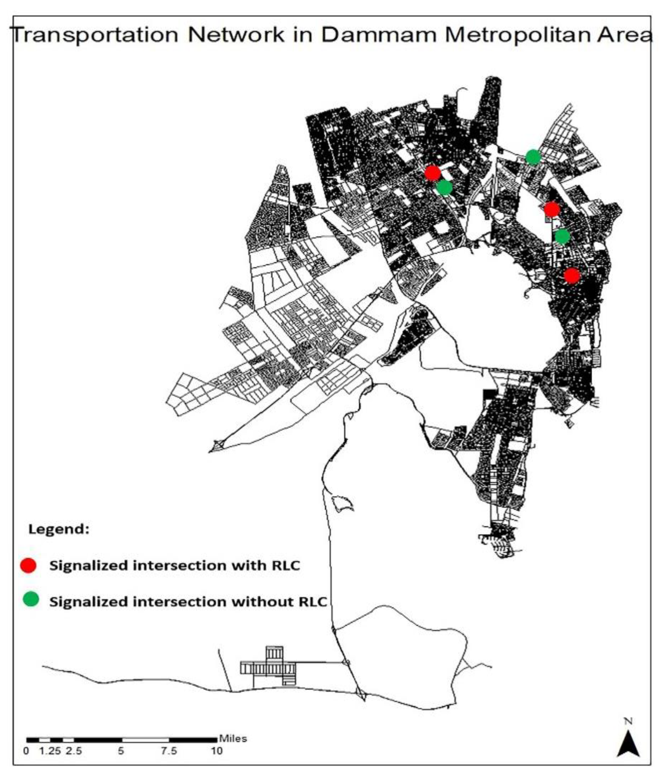
. Figure 1 shows the locations of signalized intersections where the data have been collected in DMA.

3.2. Data Collection

Data for this study were collected randomly at the above-stated intersections during morning and evening peak hours from 8 to 9 a.m. and from 4 to 5 p.m., respectively. The researcher calculated the mean of the two peak hours. The total time of collected data is about 21 h, with 7727 private vehicular headways and 311 cycles at six intersections in DMA. For each observed cycle, researchers ensured that there was a queue of ten or more vehicles without the presence of heavy vehicles. Thus, locations were chosen at six dense traffic intersections to ensure the adequate required number of vehicles in the queue. The first location includes three signalized intersections with RLCs. The first intersection with RLCs is on an arterial roadway with active land use around it, generating heavy traffic. The second and third intersections with RLCs are on a collector roadway with active land use, exhibiting a heavy traffic flow.

The second location without RLCs includes three signalized intersections, where the first and second intersections without RLCs are on an arterial roadway with active land use nearby, while the third intersection without RLCs is on a collector roadway with active land use around. The data have been collected, recorded on one approach of three or two lanes (mid-through lane) in real time at all intersections by two observers, and registered with the Excel code of vehicular trajectory and headways.

The data collection of this study followed the Highway Capacity Manual 2000 (HCM 2000) (National Research Council Transportation Research Board 2000), in which data reduction and SLT extraction were carried out from the first four vehicles’ headway in the queue after accurate estimations of headway saturation. According to HCM [19], saturation headway is only located between the fifth to the tenth vehicle in the queue (National Research Council Transportation Research Board 2000). Figure 2 shows the SLT and saturation headway in HCM [19].

The Figure 2 shows that according to the definition of SLT in HCM [19], SLT can be calculated by extracting the additional time of the first five headway vehicles from the estimated saturation headway (5th–10th vehicle in the queue) of each cycle. The study relied on Equations (2)–(4); the SLT from saturation headways only extracted the useful cycles (without the presence of heavy vehicles). The useful cycles for data collection are the signal cycles in the queue with ten or more vehicles. The chosen signalized intersections have the following common characteristics:

• Dense traffic locations;
• No grade;
• No bicycles;
• 240 s cycle length;
• No exclusive turn bays or lanes;
• Headways were measured during unsaturated conditions but with significant queues of at least ten vehicles per cycle;
• Lane width of 3.6 meters (12 feet);
• The single approach during green for each leg at a four-leg signalized intersection;
• No parking at the time of data collection;
• No buses stopping within 75 meters (250 feet) of the intersection;
• No pedestrian.

Accordingly, the saturation flow rate required no adjustments during by-cycle, prevailing conditions. The type of data reduced from the videos involved the following:

• Before the first heavy vehicle arrived for prevailing saturation headway (that is, the effects of heavy vehicles from saturation headway were removed by only queues without heavy vehicles);
• SLT data have been extracted by subtracting the headway of 1st–4th vehicle in the queue from the saturation headway of the fifth–tenth vehicles in the queue.

3.3. Data Extraction and Analysis

The data included the time headways between successive vehicles on one mid-through lane approach of 240 s cycle length. The time headways were recorded before the presence of any heavy vehicles and extracted from the 5th to 10th vehicles in the queue. Thus, the saturation headway samples and extracted SLT from the time headways are 311 from all cycles and for each location type of signalized intersections in this study (with RLCs and without).

The data have been analyzed for each location separately due to different city-wide spatial land use in DMA. Another study could be conducted to identify the impact of land use patterns on signalized intersection capacity.

4. Results

Table 2. The descriptive analysis of the first vehicle reaction time; sample by location type and intersection position.

Location Type	Intersection Position Name	Sample Size (Cycle)	First Vehicle Reaction Time (FVRT) in Seconds
			Mean	Med.	St.Dev	Min	Max	Kolmogorovs Test of Normality (Sig)
With RLCs	Harley	25	4.03	4.1	1.3	1.66	6.58	0.2
	Saad	22	4.5	4.4	1.6	1.5	7.99	0.16
	Herfy	25	4.28	3.9	1.7	1.69	7.29	0.189
	Total (1)	72	4.27	4.12	1.5	1.5	7.99	0.2
Without RLCs	Danube	52	3.48	3.33	1	1.5	5.93	0.2
	Jarash	115	3.8	3.75	1.1	1.48	6.87	0.2
	Minaa	72	3.64	3.75	1	1.7	5.8	0.2
	Total (2)	239	3.68	3.69	1.1	1.48	6.87	0.2
Total (1) + (2)		311	-	-	-	-	-	-
Histogram and normal distribution curve of the total sample size by location type
With RLCs				Without RLCs

Source: First vehicle reaction time data.

and

Table 3. The descriptive analysis of the SLT; sample by location type and intersection.

Location Type	Intersection Position Name	Sample Size (Cycle)	In Seconds Start-Up Lost Time (SLT)
			Mean	Median	St. Dev	Min	Max	Kolmogorov’s Test of Normality (Sig)
With RLCs	Harley	25	3.43	3.45	0.97	1.3	5.32	0.08
	Saad	22	3.86	3.97	1.8	0.81	0.81	0.2
	Herfy	25	3.64	3.4	1.9	0.57	0.57	0.2
	Total (1)	72	3.63	3.59	1.6	0.57	0.57	0.099
Without RLCs	Danube	52	2.37	2.2	1.3	0.31	0.31	0.2
	Jarash	115	3	3.1	1.4	0.31	0.31	0.07
	Minaa	72	2.55	2.6	1.3	0.32	0.32	0.2
	Total (2)	239	2.73	2.69	1.4	0.31	5.7	0.057
Total (1) + (2)		311	-	-	-			-
Histogram and normal distribution curve of the total sample size by location type
With RLCs				Without RLCs

Source: SLT data analysis.

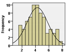
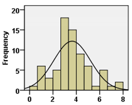
include a descriptive analysis of FVRT and SLT at the study locations. Table 2 shows that the mean and median of FVRT at the locations with RLCs are 4.27 and 4.12 s, respectively, with a standard deviation of about 1.5 s, indicating that the dispersion of the values around their mean is low or moderate. In addition, the data distribution of FVRT exhibits normality for each intersection and for the total, where the values of the Sig of Kolmogorov᾿s test of normality were greater than 5%, as shown in the histogram and normal distribution curve.

In contrast, the mean and median FVRT at locations without RLCs are lower, amounting to 3.68, and 3.69 s, respectively, with a standard deviation of about 1.1 s. This indicates that the dispersion of the values around their mean is low or moderate. Additionally, the data distribution of FVRT exhibits normality for each intersection and for the total, where the value of the Sig of Kolmogorov᾿s test of normality was greater than 5%, as exhibited in the histogram and normal distribution curve.

To sum up, the FVRT at intersections with RLCs is greater than at intersections without RLCs; thus, the RLCs at intersections with SLT will be greater than at intersections without RLCs (Table 3).

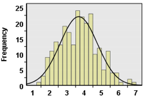
Table 3 shows that the mean and median SLT at locations with RLCs are 3.63, and 3.59 s, respectively, with a standard deviation of about 1.6 s, indicating that the dispersion of the values around their mean is low or moderate. In addition, the data distribution of SLT exhibits normality for each intersection and for the total, where the value of the Sig of Kolmogorov᾿s test of normality was greater than 5%, as illustrated by the histogram and normal distribution curve.

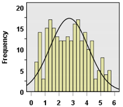
At locations without RLCs, the mean and median SLT amounted to 2.73 and 2.69 s, respectively, with a standard deviation of about 1.4 s, indicating that the dispersion of the values around their mean is low or moderate. Additionally, the data distribution of SLT exhibits normality for each intersection and for the total, where the value of the Sig of Kolmogorov᾿s test of normality was greater than 5%. This is evident from the graph of the histogram and normal distribution curve.

Based on these results and according to the Highway Capacity Manual HCM [15], the capacity of signalized intersections with RLCs is lower than the capacity of the intersections without RLCs. This may be due to the presence of RLCs.

This supports the first hypothesis of the study that there is always a trade-off between traffic safety and roadway capacity of interrupted and uninterrupted flow facilities.

Based on the results of the descriptive statistical analysis of FVRT and SLT referred to in Table 2 and Table 3, it was observed that an increase in time consumed by the first few vehicles to respond to the change in signal from red light to green increases SLT. The reported increase is higher at locations with RLCs than the surge at intersections without RLCs. Accordingly, the saturation flow rate decreases, which supports the second hypothesis inferring that an increase in SLT at the intersections with RLCs increases safety and decreases the capacity of signalized intersections.

4.1. Assessing the Correlation and Regression Analysis of the Total First Vehicle Reaction Time and Total Start-Up Lost Time for Intersections with a Red-Light Camera and without

Undoubtedly, many factors may have a significant influence on urban signalized intersections on the total SLT. The factors include the following: the presence of RLCs, response of the vehicle driver, number of lanes and width of each one, operational efficiency of the vehicle, demographic characteristics of vehicle drivers, weather condition, the structural condition of the road, number of vehicles and pedestrians that still cross the road inside the intersections after the signal is opened, and others. But the current study focuses on studying the impact of one factor only. It investigates the presence of RLCs at urban signalized intersections by studying the impact of total first vehicle reaction time FVRT on total start-up lost time SLT for intersections with a red-light camera and without.

Typically, the logical correlation between FVRT and SLT is positive, as each increase in FVRT leads to a proportional impact on SLT. To study the effect of FVRT (independent variable) on the SLT (dependent variable), a simple regression will be analyzed to formulate a regression model that is utilized to predict the SLT based on FVRT. This analysis is carried out after verifying the statistical significance of the model and its coefficients, as well as confirming the model's assumptions, such as linearity and normality.

4.1.1. Assessing the Correlation and Regression Analysis of Total First Vehicle Reaction Time on Total Start-Up Lost Time at the Intersections with a Camera

H₀ 

: There is no significant effect of FVRT on SLT at urban signalized intersections with RLCs.

H₁: 

There is a significant effect of FVRT on SLT at urban signalized intersections with RLCs.

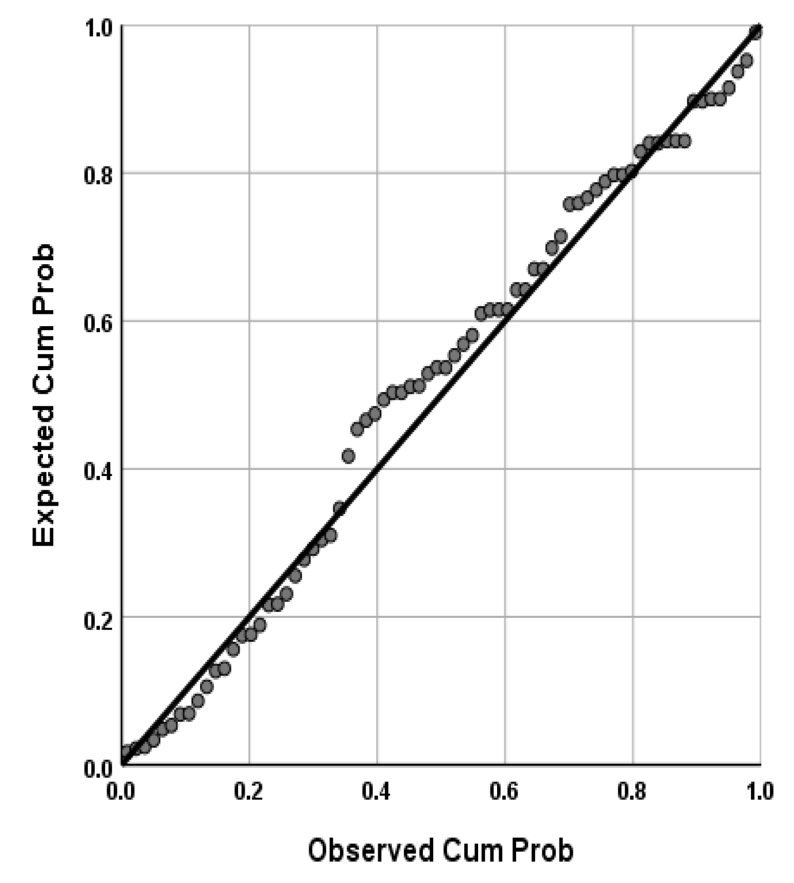
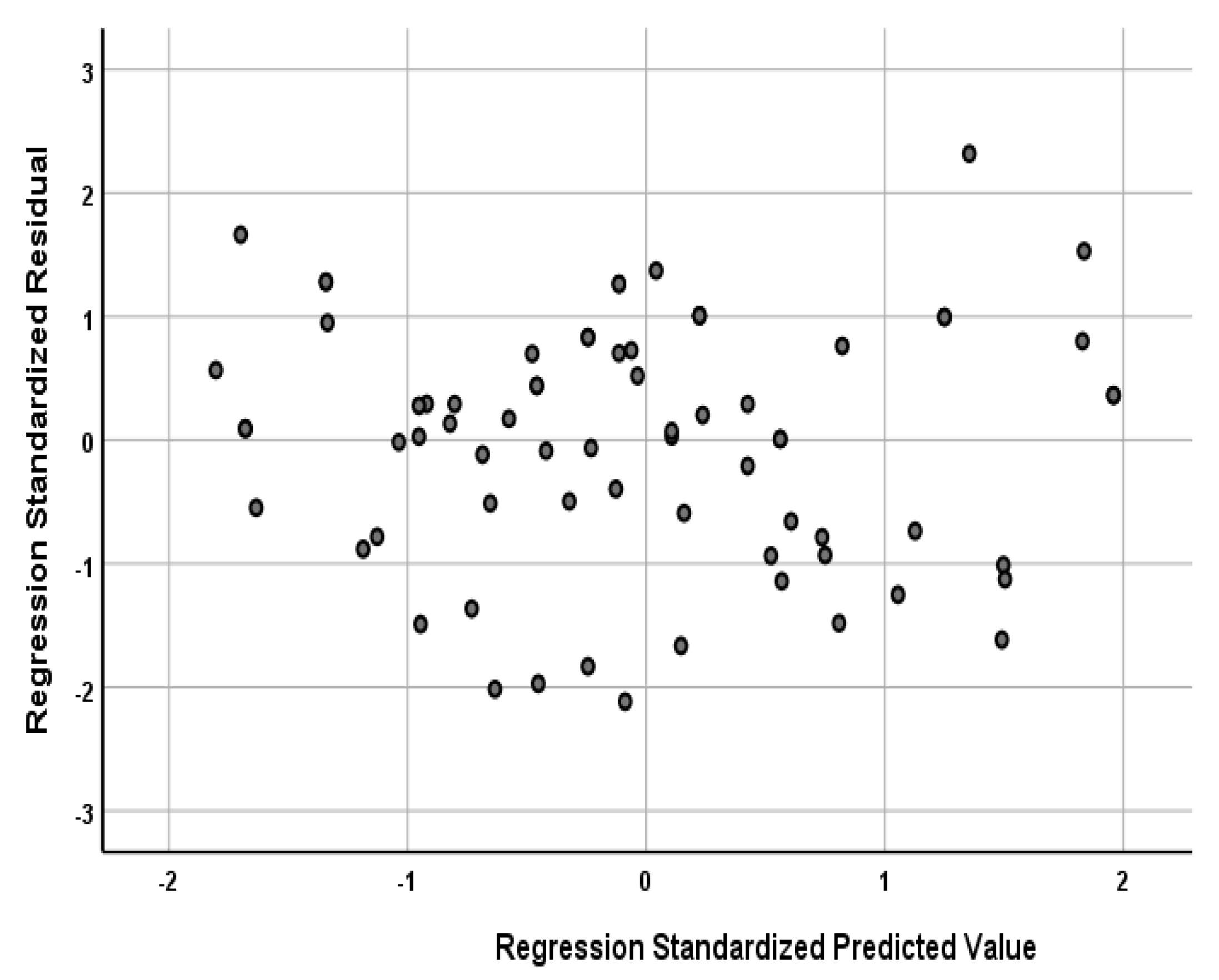
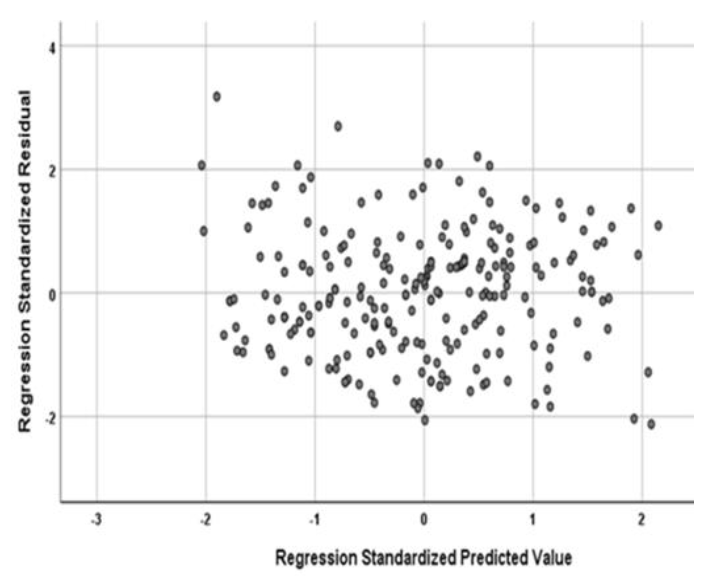
Simple regression analysis between the independent FVRT variable and dependent SLT variable shows that the best mathematical model with statistical significance at a significant level of 0.01 for the model and its coefficients is the linear model. A logical correlative relationship between the two variables was obtained, as shown in

Table 4. Regression Analysis of the total first vehicle reaction time on total start-up lost time at the intersections with cameras.

Equation No	Equation	R2	R	Std. Error of the Estimate	F
(7)	ŷ1= 0.782 + 0.667 X1 (1.9) (7.2) **	0.43	(0.65) **	1.2	(52.2) **
The structural formula of the logic mathematical linear model is “ Y1 = a1 + b1X1 “, where the following is the case: - Y1 is the dependent variable (SLT); - X1 is the independent variable (FVRT); - a1 is a constant value = 0.782; - b1 is the coefficient of X1 that is called regression coefficient = +0.667; - The positive sign (+) relates to the positive relationship between the two variables; - The value between the brackets below the equation indicates the value of t statistics for the coefficients of the linear model. - ( ) ** is significant at level 0.01, and ( ) is not significant.

Source: Output sheet of simple regression analysis by SPSS 25.0 (2017).

. Moreover, the assumptions of the model were verified, as shown in Figure 3 and Figure 4.

The indicators of the simple regression analysis revealed the following:

• The value of the coefficient of determination (R2) amounted to about 0.43, which means that only 43% of the change in the SLT is due to the change in the FVRT. About 57% of the change in the SLT is due to the influence of other factors that are not measured. In addition, Pearson’s correlation coefficient (R) is 0.65, which indicates the mid and positive linear correlation between the SLT and FVRT. To the low value of the Std., the error of the estimate amounted to 1.2.
• The value of F indicates the significance of the model as a whole (significance level of 0.01).
• The regression coefficient (b1 = +0.667) means that each increase in the FVRT by one second will increase the SLT by 0.667 s and vice versa.

Based on the above-mentioned, the alternative hypothesis (H1) is accepted. Thus, the model can be used for predicting the SLT according to the changes in FVRT at a confidence degree of 99%, considering that only 43% of the change in SLT is the responsibility of the change in FVRT, with a moderate impact. This confirms that there are other unmeasured factors affecting SLT at urban signalized intersections other than the presence of RLCs.

4.1.2. Assessing the Correlation and Regression Analysis of Total First Vehicle Reaction Time on Total Start-Up Lost Time at the Intersections without a Camera

H₀ 

: There is no significant effect of FVRT on SLT at urban signalized intersections without RLCs.

H₁: 

There is a significant effect of FVRT on SLT at urban signalized intersections without RLCs.

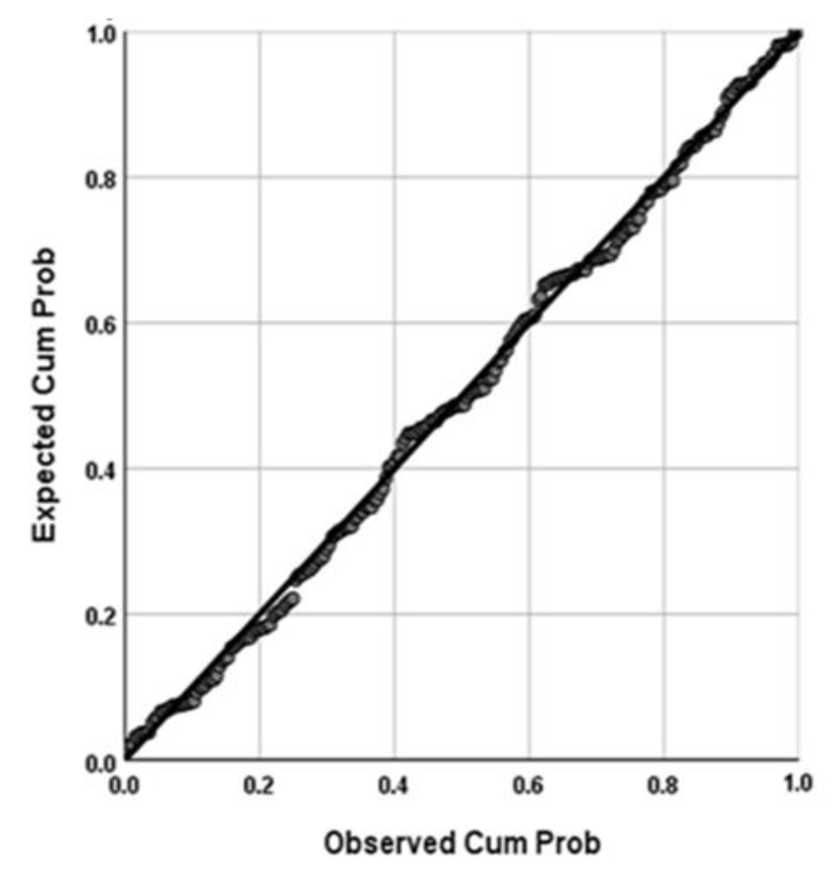
Between the independent variable and the dependent variable, simple regression analysis shows that the best mathematical model with statistical significance at a significant level of 0.01 for the model and its coefficients is the linear model. Additionally, it achieves the logical correlative relationship between the two variables, as shown in

Table 5. Regression analysis of total first vehicle reaction time on total start-up lost time at the intersections without a camera.

Equation No	Equation	R2	R	Std. Error of the Estimate	F
(8)	ŷ2= 0.287 + 0.664 X2 (1.1) (9.4) **	0.27	(0.52) **	1.18	(88.1) **
The structural formula of the logic mathematical linear model is “ Y2 = a2 + b2X2 “, where: - Y2 is the dependent variable (SLT); - X2 is the independent variable (FVRT); - a2 is a constant value = 0.287; - b2 is the coefficient of X2 that called regression coefficient = 0.664; - The positive sign (+) refers to the positive relationship between the two variables; - The value between the brackets below the equation indicates the value of T for the coefficients of the linear model; - ( ) ** is significant at level 0.01, and ( ) is not significant.

Source: Output sheet of the simple regression analysis by SPSS.

following equation No (8). The assumptions of the model were verified, as shown in Figure 5 and Figure 6.

The indicators of the simple regression analysis yield the following outputs:

• The value of the coefficient of determination (R2) is about 0.27, which means that only 27% of the change in the SLT is due to the change in the FVRT. About 73% of the SLT has changed due to the influence of other factors that are not measured. Pearson’s correlation coefficient (R) amounted to about 0.52, which indicated the mid and positive linear correlation between the SLT and FVRT. In addition to the low value of Std., the error of the estimate amounted to 1.18.
• The value of F indicates the significance of the model as a whole (p = 0.01).
• The regression coefficient (b2 = +0.664) means that each increase in the FVRT by one second will increase the SLT by 0.664 s and vice versa.

Based on the above-mentioned, the alternative hypothesis (H1) is accepted, which assumed that the FVRT has a significant effect on the SLT at a significant level of 0.01. Thus, the model can be used for predicting the amount of the SLT according to the changes in FVRT at a confidence degree of 99%, considering that only 27% of the change in SLT is the responsibility of the change in FVRT, which exhibits a low impact that corresponds to the study's assumptions.

4.1.3. The Expected Start-Up Lost Time Corresponding to the Changes in the First Vehicle Reaction Time for Each Location

Table 6. The expected value of start-up lost time SLT per cycle and per peak hour according to the changes in the first vehicle reaction time FVRT by the location type.

Location Type	Equation of Simple Linear Regression	Independent Variable (X) Dependent Variable (Y)	Changes of (FVRT) in Seconds
			1	2	3	4
With RLCs	ŷ1 = 0.782 + 0.667 X1	the expected value of (SLT) in seconds/cycle (Y1)	1.45	2.12	2.78	3.45
		the expected value of (SLT) in seconds/peak hour	21.75	31.8	41.7	51.75
Without RLCs	ŷ2 = 0.287 + 0.664 X2	the expected value of (SLT) in seconds/cycle (Y2)	0.95	1.62	2.28	2.94
		the expected value of (SLT) in seconds/peak hour	14.25	24.3	34.2	44.1
the difference between the expected value of (SLT) in seconds/peak hour at locations with RLCs and without RLCs = (ŷ1 × 15 cycles) − (ŷ2 × 15 cycle)			7.5	7.5	7.5	7.65
Percentage increase (%) in the expected value of (SLT) in seconds/peak hours at a location with RLCs to the expected value of (SLT) in seconds/peak hours at a location without RLCs			51.6	30.9	21.9	17.3
where: - The average time per cycle during peak hours is approximately 240 s for each location; - The number of cycles during one peak hour = 3600/240 = 15 cycles/one peak hour; - X1 = X2 = changes in FVRT in seconds from 1 to 4. - By knowing the changes in FVRT, the expected value of SLT in seconds/cycle was calculated from the simple linear regression equation that was estimated for each location.

indicates that an increase in FVRT from 1 to 4 s increases the expected value of SLT from 21.75 to 51.75 s and from 14.25 to 44.1 s during the peak hour at the intersections with RLCs and without RLCs, respectively. It is noted that total SLT at the intersections with RLCs is always greater than the total SLT at the intersections without RLCs. The difference between them gradually increased from 7.5 to 7.65 s during peak hours. However, this gradual increase at a low rate amounted to 51.6% as the maximum and decreased gradually to 17.3% as the minimum. This is due to the presence of some other SLT factors affecting both locations. This confirms the need for the impact of other factors to study the SLT, and this will be carried out later.

4.2. Analysis of Variance (ANOVA) for the Means of the Study Variables

To examine the existence of significant differences among the means for each variable by intersection position and by location type, ANOVA was conducted to verify some hypotheses and answer some questions:

• Does the difference in intersection positions per location have a significant effect on the means of the variables of the study? Therefore, this hypothesis per location is as follows:

H₀ 

: There is no significant effect of the intersection position on the values of study variables.

H₁ 

: There is a significant effect of the intersection position on the values of study variables.

• Does the difference in location type (with a camera and without a camera) have a significant effect on the means of the variables of the study? Therefore, this hypothesis is as follows.

H₀: 

There is no significant effect of the location type on the values of study variables.

H₁ 

: There is a significant effect of the location type on the values of study variables.

For the study, it is necessary to verify the homogeneity of the variance of the variables' values to determine the appropriate analysis of the variance test as a parametric ANOVA test or nonparametric Kruskal–Wallis test. This is based on the result of Levene’s test for homogeneity.

4.2.1. ANOVA Test for the Study Variables at Intersections with Cameras

Depending on the result of Levene’s test, one-way ANOVA and Kruskal–Wallis tests were conducted for FVRT and SLT, respectively, among three intersections, as shown in

Table 7. Results of analysis of variance among three intersection positions with camera for the study variables (first vehicle reaction time and start-up lost time).

Intersection Position Name	Mean (In Seconds)	Variable	Levene’s Test		Results of Analysis of Variance
			Value	Sig	Test Type	Chi-Square Value	F Value	Sig
Harley	4.03	first vehicle reaction time (FVRT)	0.79	0.46	One-way-ANOVA		0.63	0.53
Saad	4.5
Herfy	4.28
Harley	3.43	Start-up lost time (SLT)	12.7	0.00	Kruskal–Wallis	0.651	-	0.72
Saad	3.86
Herfy	3.64

Levene test: The variance of each intersection is equal if Sig and gt is 0.05, and vice versa. Analysis of variance: There is no significant difference between the means if Sig and gt is 0.05, and vice versa. Source: Output sheet of analysis of variance test by SPSS.

. This indicates that there are no significant differences among the means of FVRT and SLT at the three intersections, where the value of Sig. was greater than 5% for each one that amounted to 0.53 and 0.72, respectively. Therefore, we will accept the null hypothesis (H0) stating that there is no significant effect of the intersection position on the values of study variables and reject the hypothesis (H1).

4.2.2. ANOVA Test for the Study Variables at Intersections without the Camera

Table 8. Results of analysis of variance among three intersection positions without the camera for the study variables (first vehicle reaction time and start-up lost time).

Intersection Position Name	Mean (In Seconds)	Variable	Levene Test		Results of Analysis of Variance
			Value	Sig	Test Type	F Value	Sig
Danube	3.48	first vehicle reaction time (FVRT)	0.51	0. 6	ANOVA	1.64	0.195
Jarash	3.8
Minaa	3.64
Danube	2.37	start-up lost time (SLT)	0.97	0.38	ANOVA	4.78	0.009
Jarash	3
Minaa	2.55

Levene test: The variance of each intersection is equal if Sig > 0.05, and vice versa. Analysis of variance: There is no significant difference between the means if Sig > 0.05, and vice versa. Source: Output sheet of the one-way ANOVA test by SPSS.

indicates that there are no significant differences among the means of FVRT at the three intersections, where the value of Sig. was greater than 5%, which amounted to 0.195. Therefore, we will accept the null hypothesis (H0), assuming that there is no significant effect of the intersection position on the values of FVRT and reject the alternative hypothesis (H1). There is a significant difference among the means of the SLT variable at the three intersections, where the value of Sig. was smaller than 5%, which amounted to 0.009. It leads to the rejection of the null hypothesis (H0) and the acceptance of the alternative hypothesis (H1).

4.2.3. ANOVA Test for the Study Variables According to the Location Type

Depending on the result of Levene’s test, Kruskal–Wallis and ANOVA tests were conducted for FVRT and SLT, respectively, between two locations, as shown in

Table 9. Results of analysis of variance between two locations for the study variables (first vehicle reaction time and start-up lost time).

Mean of Variables by Location Type (In Seconds)		Variable	Levene’s Test		Results of Analysis of Variance
With Camera	Without Camera		Value	Sig	Test Type	Chi-Square Value	F Value	Sig
4.27	3.68	Total first vehicle reaction time (FVRT)	13.4	0.000	Kruskal–Wallis	8.3	-	0.004
3.63	2.73	Total start-up lost time (SLT)	0.11	0.74	One-way ANOVA	-	22.36	0.000

Levene test: The variance of each location is equal if Sig > 0.05, and vice versa. Analysis of variance: There is a significant difference between the means if Sig < 0.05, and vice versa. Source: Output sheet of the analysis of variance test by SPSS.

. This indicates that there are significant differences between the means of the two variables (FVRT and SLT) at the two locations. The value of Sig. was smaller than 5% for them, which amounted to 0.004 and 0.000 for each, respectively. Therefore, we will reject the null hypothesis (H0) and accept the alternative hypothesis (H1), showing a significant effect of the location type on the values of FVRT and SLT.

In Table 7, Table 8 and Table 9, the significant differences between locations in similar categories are related to differences in signalized intersection locations and roadway classifications. The first location with RLCs is a signalized intersection on an arterial roadway with surrounding active land use. The second and third locations with RLCs are on collectors with surrounding active land use. The first and second locations without RLCs are on arterial roadways with active land use around, while the third location without RLCs is on a collector roadway with surrounding active land use. These differences assist the correlation of other factors to FVRT and SLT.

5. Conclusions

The study revealed a significant increase in start-up lost time (SLT) for the first few vehicles at signalized intersections when transitioning from a red light to a green light. The presence of red-light enforcement cameras (RLCs) at intersections is associated with a higher SLT compared to intersections without RLCs, resulting in a decrease in saturation flow rate. These findings support the main hypothesis of the study, indicating that RLCs at intersections contribute to increased safety but reduce the overall capacity of signalized intersections. Furthermore, it is concluded that intersections with RLCs exhibit higher first-vehicle reaction time (FVRT) than intersections without RLCs. This highlighted the impact of RLCs on SLT. The findings of this study contribute to the academic literature by providing empirical evidence on the relationship between RLCs, SLT, and FVRT at signalized intersections. The identified correlation between FVRT and SLT, supported by the existing literature on driver characteristics, enhances the understanding of the complex dynamics of signalized intersections. Moreover, the study pinpointed the need for further investigations into additional influencing factors, particularly when drivers’ behavior differs significantly from the established guidelines. RLCs are effective at reducing right-angle crashes, right-angle injury crashes, and total injury crashes. However, they also appear to increase rear-end crashes. RLCs can reduce crashes under some conditions, but on the whole, RLCs do not seem to be a successful safety measure. The implication of the study contributes widely to societal transport development. The control of the crashes in the metropolis area with urban and signalized intersection zones required both red-light cameras and red-light countdowns to rectify the SLT and FVRT's increased seconds. Providing a countdown signal to reduce FVRT, SLT, and total lost time is highly recommended. As the study's results show the identified acceptance of the hypothesis about the significant effects of RLCs on the approaches of FVRT and SLT. The analysis of the study shows substantial recommendations for future researchers to overlook transport science development with red-light camera enforcement and red-light countdown to control the chances of crashes and accidents. It is important to acknowledge certain limitations in this study. Firstly, the research was conducted in the specific context of the studied metropolitan area, and the findings may not be directly generalizable to other regions or jurisdictions. Additionally, the study focused solely on the impact of RLCs on SLT and capacity without considering other potential variables that could affect intersection performance. Future research should address these limitations by conducting studies in diverse settings and incorporating a broader range of factors influencing intersection dynamics. Future research should explore the combined effects of RLCs and countdown signals at signalized intersections. Investigating the correlation between FVRT and SLT in the presence of RLCs while considering additional factors, such as driver characteristics and behavior, will provide a more comprehensive understanding of intersection operations. Furthermore, examining the effectiveness of alternative measures, such as countdown signals, in reducing FVRT, SLT, and total lost time is crucial for improving intersection efficiency and safety.