Article

Analyzing Driving Safety on Prairie Highways: A Study of Drivers’ Visual Search Behavior in Varying Traffic Environments

1
School of Energy and Transportation Engineering, Inner Mongolia Agricultural University, Hohhot 010018, China
2
Faculty of Social Science and Public Policy, King’s College London, London WC2R 2LS, UK
*
Author to whom correspondence should be addressed.
Sustainability 2023, 15(16), 12146; https://doi.org/10.3390/su151612146
Submission received: 12 June 2023 / Revised: 2 August 2023 / Accepted: 7 August 2023 / Published: 8 August 2023

Abstract

:
This study aimed to investigate disparities in drivers’ visual search behavior across various typical traffic conditions on prairie highways and analyze driving safety at the visual search level. The study captured eye movement data from drivers across six real-world traffic environments: free driving, vehicle-following, oncoming vehicles, rear vehicles overtaking cut-in, roadside risks, and driving through intersections, by carrying out a real vehicle test on a prairie highway. The drivers’ visual search area was divided into five areas using clustering principles. By integrating the Markov chain and information entropy theory, the information entropy of fixation distribution (IEFD) was constructed to quantify the complexity of drivers’ traffic information search. Additionally, the main area of visual search (MAVS) and the peak-to-average ratio of saccade velocity (PARSV) were introduced to measure visual search range and stability, respectively. The study culminated in the creation of a visual search load evaluation model that utilizes both VIKOR and improved CRITIC methodologies. The findings indicated that while drivers’ visual distribution and transfer modes vary across different prairie highway traffic environments, the current lane consistently remained their primary area of search for traffic information. Furthermore, it was found that each visual search indicator displayed significant statistical differences as traffic environments changed. Particularly when encountering roadside risks, drivers’ visual search load increased significantly, leading to a considerable decrease in driving safety.

1. Introduction

As road traffic motorization continues to accelerate, traffic safety issues are becoming increasingly prominent [1,2]. Within the people–vehicle–road system, the driver plays a crucial role, but is also the system’s most vulnerable link [3,4]. Traffic accident causation analysis reveals that human factors contribute to as many as 93% of traffic accidents [5]. Among these human factors, vision plays a dominant role, with over 90% of traffic environment information during driving being obtained through the driver’s visual search [6,7]. Therefore, it is essential to investigate the relationship between traffic environments and drivers’ visual search behavior from a visual psychological safety perspective.
In the realm of traffic human factors engineering, research has been conducted on drivers’ visual search behavior in various traffic environments [8,9,10,11,12,13]. Sun et al. [14] presented a gaze-based integrated driving assessment method and found notable differences in visual search modes of elderly drivers at roundabouts and intersections. Stahl et al. [15] constructed three different conflict scenarios for driving simulation experiments, verifying general differences in visual search patterns between novice and experienced drivers in relation to recognizing meaningful cues in specific scenarios. Lemonnier et al. [16] conducted real vehicle tests on rural roads, demonstrating that priority rules, anticipated traffic density, and the number of intersection passages all affect drivers’ visual attention. Qin et al. [17] created a mountainous low-grade highway scenario for driving simulation tests, identifying differences in drivers’ visual search behavior across five typical road sections. Li et al. [18] studied drivers’ visual scanning behavior at various intersections, discovering significant differences in information search modes at signalized and unsignalized intersections. Wu et al. [19] studied the influence of vehicle cut-in on the stability of following vehicles, indicating that when the vehicle cuts in, the driver’s visual information search range remained focused on the field of front vision, but the attention to the emergence direction of the cut-in vehicle increased. Yuan et al. [20] conducted a real vehicle experiment on typical urban roads and found that drivers were more distracted when driving on relatively complex road sections, and the horizontal search width reached a maximum at intersections.
A good visual search mode is the premise for drivers to obtain useful and high-quality visual information from the traffic environment promptly, ensuring early detection, judgment, and decision-making of potential dangers during driving to adjust driving strategies and behaviors to ensure safe vehicle operation [8,21]. When the driver is in a complex traffic environment, the amount of information to be received and processed increases, and the visual resources consumed to search for driving information in the traffic environment increase. When the visual search load borne by the driver reaches the limit, insufficient or untimely information search may occur, resulting in dangerous driving behaviors such as slow reaction or misjudgment, and reduced driving safety [22,23,24,25].
Prairie highways, a unique segment of road traffic, are constrained by environmental factors such as terrain and landforms. Current prairie highways typically lack central medians and roadside guardrails, coupled with the complexity and diversity of vehicle types and the discrete distribution of speed, highlighting a series of characteristics such as backward traffic safety facilities and a low management level [26,27]. The driving process on such highways is often affected by opposing traffic flows and the roadside environment, leading to more chaotic traffic orders compared to other road environments. In addition, due to the simple line shape of prairie highways, the monotonous roadside landscape, and the insufficient number and information quantity of traffic signs, they can easily cause the phenomenon of road hypnosis, which causes the dynamic visual fatigue of drivers and decreases their ability to perceive and process information [28]. When the traffic environment changes suddenly during driving, the driver’s search and perception demand for visual information increases instantaneously, affecting the driver’s visual information search mode, leading to incorrect driving judgments and decisions, and thereby impacting driving safety.
In recent years, the research on driving safety of prairie highways from the perspective of human-factor safety has mainly focused on fatigue driving, traffic facilities information, and road alignment design. In terms of fatigue driving, Peng et al. [29] built a prairie highway scenario for simulated driving tests to explore the generation mechanism of fatigue driving, extracted the driver’s operational response and ECG data, constructed an effective indicator set to measure the degree of driving fatigue, and classified the fatigue driving state into three types: mild, moderate, and severe. Zhang et al. [27] conducted a real driving test on prairie highways, studied the relationship between drivers’ EEG and driving time, and divided driving fatigue into stages from the time dimension. Liu et al. [30] found that paving colored pavements on prairie highways helps to alleviate drivers’ subjective fatigue and keeps them well alert and responsive. For the research on traffic facility information, Li Hangtian et al. [28] and Li Xiaoju et al. [31] designed virtual scenarios of prairie highways with different amounts of traffic facility information for a simulated driving test and studied the effect of traffic facility information on drivers’ visual information processing mode. They determined the optimal information thresholds conducive to driving safety based on the performance of drivers’ visual search ability. In terms of road linear design, Wang et al. [32] used a typical desert prairie highway as a test section to conduct an eye-movement tracking test of drivers and analyzed the range of distance values for long straight road sections conducive to driving safety from the perspective of visual search stability.
In summary, previous studies have found that drivers’ visual search behavior is influenced by the traffic environment, but there are few detailed and in-depth quantitative analyses of its influence degree, and there is still a lack of research related to the visual search behavior of drivers in different traffic environments on prairie highways from the perspective of human-factor safety. The real vehicle test has a certain exploratory value for driving safety research because it highly restores the road scene and driving environment, which enables drivers to exhibit more natural driving behaviors and risk perceptions [33,34,35]. In light of this, this study employed a real vehicle test on a prairie highway to collect drivers’ eye movement data under six traffic environment conditions: free driving (FD), vehicle-following (VF), oncoming vehicles (OV), rear vehicles overtaking cut-in (RVOC), roadside risks (RR), and driving through intersections (DTI). We constructed an evaluation indicator system from the perspectives of visual search complexity, stability, and visual field range. Based on multi-featured visual indicators, we explored the differences in drivers’ visual search behaviors under varying traffic environments. By integrating weight theory, we created a visual search load evaluation model to analyze driving safety on prairie highways at the visual search level.
In this study, we proposed the following hypotheses:
  • Different types of traffic environments influence drivers’ visual distribution and transfer modes;
  • An increase in environmental elements along both sides of the road intensifies the difficulty of obtaining visual information and broadens the driver’s visual search range;
  • An increase in traffic environment information expedites the driver’s visual search behavior, often resulting in decreased visual stability.
This study holds substantial theoretical significance for correcting undesirable visual search behavior noticed in drivers on prairie highways, further investigating driving safety hazards and exploring accident causation on these highways. It can also offer theoretical guidance for driving behavior intervention and graded early warning, improvement of traffic safety facilities on prairie highways, and enhancement of traffic management levels.
The remainder of the paper is structured as follows. Section 2 details the design of the real vehicle test, the construction of visual search indicators, and the analysis methodology. Section 3 examines the drivers’ visual search behavior in different traffic environments and introduces the concept of visual search load to evaluate driving safety. Section 4 discusses and compares the research findings. Section 5 encapsulates the research results and contributions.

2. Materials and Methods

2.1. Real Vehicle Experiment

2.1.1. Experimental Road

The test road section was a second-class prairie highway on the Saihantala–Mandulatu stretch of provincial highway S101 in Xilinhot, Inner Mongolia, China. The road section was located in a plain area with a dry climate and little rain, a harsh ecological environment, and a low population density. Table 1 provides specific information about the test road section. Through field observation and inspection, the test road was a typical semi-desert prairie highway, the traffic condition of the road was in a state of free flow, and the linear design primarily consisted of long straight lines with small longitudinal slope gradients. The roadside vegetation was herbaceous plants with a low coverage rate, the landscape was monotonous and dull, and there were few villages and towns on the way. The test road is shown in Figure 1. In addition, due to insufficient traffic management, the test road had no median strip and roadside guardrail facilities, traffic signs were scarce and not systematic, the vehicle type was unrestricted, cars, heavy vehicles, tractors, and so on were allowed to pass through, but the main vehicle type was cars.

2.1.2. Experimental Participants

In order to enable the subjects to better reflect the group characteristics of drivers, based on the multiple screening criteria, 22 licensed car drivers (12 males and 10 females) were recruited as subjects to participate in the test. The subjects aged from 24 to 55 years (Mean = 34.3, SD = 9.9), and all had at least two years of driving experience (Mean = 8.2, SD = 5.5), normal hearing and visual function, no history of psychiatric disorders and experience of serious traffic accidents. In order to ensure the objectivity of data collection, the subjects were required to maintain sufficient sleep, avoid vigorous exercise and drug misuse before the test was conducted. The subjects were informed of the general conditions of the test and signed a written informed consent form.

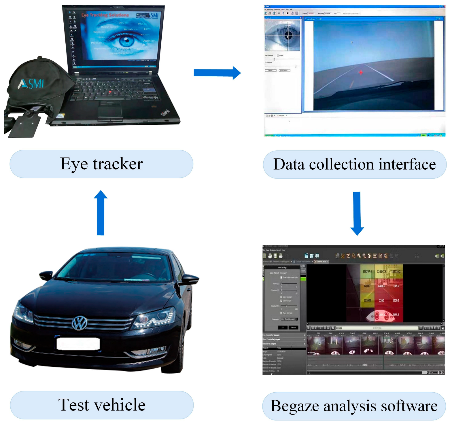
2.1.3. Experimental Equipment

The vehicle used for the test was a Volkswagen Passat automatic vehicle with good performance. The eye tracker device was selected as the IView X series head-mounted eye tracker from the SMI company in Germany, and the detailed parameters of this device are shown in Table 2. The eye tracker was connected to a dedicated laptop for acquiring, recording, and archiving eye movement data. The built-in camera of the eye tracker can record a high-resolution scenario video in real time and superimpose it with the eye movement data synchronously through the built-in processor. The scenario video and eye movement data were extracted using the self-contained software Begaze, and data screening and a preliminary analysis were performed. At the same time, an illuminance meter and a noise meter were equipped in the test vehicle to control the consistency of the test conditions. The main test equipment is shown in Figure 2. Other auxiliary equipment included cameras, calculators, 12 V DC batteries, etc.

2.1.4. Experimental Procedure

The test was conducted in September when the weather conditions were suitable. To avoid the effect of light intensity and varying traffic conditions, the test was conducted during off-peak hours from 8:00 a.m. to 11:00 a.m. in clear weather, and the test road pavement was dry without standing water. The illuminance and noise values at the primary driving position inside the vehicle were measured with an illuminance meter and noise meter, respectively, to ensure the consistency of the test environment conditions. The total length of the test road was 150 km, and the duration of each test was about 2 h. Repeated tests on the same road section for a long time were not performed to prevent familiarizing the subjects with the test environment, as this may lead to a decrease in the validity of the acquired eye movement data. In addition, considering the condition constraints of the test implementation and the safety of the personnel, all subjects were tested once. The specific procedure of the test comprised four stages: information collection, adaptability training, the formal test, and data summary.
  • Test preparation: Staff members explained the test content and process to the subjects and briefly introduced the test conditions, asking them to carefully read and fill out the written informed consent form.
  • Adaptability training: The subjects entered the test vehicle, completed the seat adjustment, and cooperated with the researchers to wear the eye tracker correctly. Subsequently, the subjects performed 10 min of actual driving training to drive the test vehicle to the starting point of the test road to adapt to the wearing of the eye tracker and driving environment and performed 5 min of static measurement of eye movement data at the starting point.
  • Formal test: The subjects drove the test vehicle to a designated destination along a planned route. They were required to control the vehicle according to their usual driving habits while adhering to traffic rules and speed limits. During the driving process, the observer continuously monitored the platform interface for recording eye movement data. If any interruption or loss in the data collection process was detected, the participant was promptly notified and asked to adjust the test equipment to ensure the quality of test data.
  • Data summary: After the test, the subjects’ basic information and eye movement data were promptly collated and summarized.

2.1.5. Data Extraction and Processing

Traffic Environment Division

We have considered the following reasons for the selection of traffic environment:
  • The test road was a typical prairie highway with a two-lane design in both directions. Due to the lack of median strip and roadside guardrail facilities, the driving process was vulnerable to the interference of opposing traffic flows and the roadside environment.
  • There were no signal controls at the intersections of the test section, and vehicles on the main road had priority. The traffic operations of the main road were disturbed by lateral traffic flows of the branch, which posed a safety hazard.
  • Limited to insufficient traffic control, the test road had complex and diverse vehicle types and discrete speed distribution, and the driving process was vulnerable to the influence of other vehicles in the same direction lane.
To eliminate the interference of road alignment, safety facilities, and other factors on the test results, the eye movement data of drivers navigating through different traffic environments on a smooth and straight road section were extracted in time units. Taking into account the road conditions, roadside environment, and traffic safety facilities of the prairie highway, the selected traffic environments include: vehicle-following (VF), oncoming vehicles (OV), rear vehicles overtaking cut-in (RVOC), roadside risks (RR), and driving through intersections (DTI). The period when no other traffic participants, roadside risks, and intersections within the driver’s field of vision was selected as the control group. This condition was defined as free driving (FD) in this study. Figure 3 depicts a schematic of the various traffic environments.
The scientific and reasonable construction of the data time window can significantly influence the precision and reliability of the research findings. Given the varying time window widths corresponding to different traffic environments, this study referred to current research findings and combined them with the objective phenomena observed during real vehicle tests on the prairie highway. The interpretation of different traffic environments and the definition of time window widths are shown in Table 3.

Data Processing

This study primarily focused on analyzing the eye movement data of participants in six traffic environments on prairie highways. After 22 drivers had completed the test in accordance with the test requirements, the data were initially screened using the Begaze analysis software to eliminate samples with severe loss and calibration bias. Consequently, the valid data of 20 subjects were retained. Based on the interpretation of different traffic environments and the selection of time window widths, the eye tracker collected videos were observed frame by frame to extract the eye movement data sets for different driving environments. We extracted a total of 1027 eye movement data sets involving 20 subjects in different driving environments and used ORIGIN, SPSS, and other software for subsequent statistics and analysis.

2.2. Area of Interest Division

During driving, owing to the variations in the density and importance of traffic information in different areas within the driver’s field of view in different traffic environments, drivers tend to have a subjective bias in their visual search mode. They often employ selective attention to repeatedly search the target information area of interest to ensure they gather adequate and effective traffic environment information, thereby ensuring driving safety [36,37]. To compare and investigate drivers’ visual search behaviors in different traffic environments, it is essential to divide the drivers’ areas of interest (AOI).
The dynamic clustering method, which has the benefits of a simple principle, ease of implementation, and the ability to gradually enhance clustering accuracy through several iterations, is frequently used in studying AOI division. For example, the K-means clustering method, owing to its simple calculations, strong applicability, efficient operation, and good scalability for large sample size datasets, has become a traditional method for AOI division [38,39,40].
We established the Euclidean distance as the criterion to measure the similarity between data, adopted the sum of squares of errors (SSE) as an objective function to gauge the clustering accuracy, and performed K-means clustering of the analytical coordinates of the fixation points on the visual field plane to divide the AOIs.

2.3. Visual Search Process Based on Markov Chain

2.3.1. Markov Chain

Let us set a sequence of random variables as { X ( t ) , t 0 } , whose discrete state space is I = i , j , i 1 if there are any nonnegative integer 0 t 1 < t 2 < < t r < m and positive integer k , such that it satisfies Equation (1).
P { X ( m + k ) = j X ( t 1 ) = i 1 , X ( t 2 ) = i 2 , , X ( t r ) = i r , X ( m ) = i } = P { X ( m + k ) = j X ( m ) = i }
Here, { X ( t ) , t 0 } is called the Markov chain.
The Markov chain is a random process with discrete time and state and typically no after-effect. When the state of the process at time m is known, the state of the process at time m + k is only related to the state condition at time m but not to the state of the process before time m [41]. The transfer process of the driver’s fixation point is regarded as a state transition, where the fixation point falls into different AOIs classified as different states. The AOI of the next fixation point is only related to the state of the current fixation point, and the time and state are discrete, which conform to the characteristics of the Markov chain. Therefore, the Markov chain theory can be used to study the transfer process of the driver’s fixation point [41,42,43].

2.3.2. One-Step Transition Probability Matrix of Fixation Points

For the Markov chain { X ( t ) , t 0 } , the conditional probability p i j ( m , m + k ) represents the transition probability of the Markov chain from state i at time m to state j at time m + k , as shown in Equation (2).
P { X ( m + k ) = j X ( m ) = i } = p i j ( m , m + k )
The transition probability p i j ( m , m + k ) is denoted as p i j ( k ) ; then, when k = 1 , p i j ( 1 ) is the one-step transition probability of the Markov chain, denoted by p i j . If the driver’s visual search area is divided into n AOIs, the drivers’ fixation point transfer process can be regarded as a Markov chain with state space I = 1 , 2 , , n , and the one-step transition probability matrix P of the fixation points is constructed as follows:
P = p i j n × n = p 11 p 12 p 1 n p 21 p 22 p 2 n p n 1 p n 2 p n n
The one-step transition probability of the fixation points between each AOI is then calculated. According to the principle of statistical estimation, when the sample size is large enough, the theoretical distribution of states can be described approximately by the sample distribution, and the transition probability can be estimated approximately by the transition frequency [44]. The transition probability p i j of fixation points from state i to state j is shown in Equation (4):
p i j = a i j a i
where p i j 0 and j I p i j = 1 ; j I a i j = a i , a i j represents the frequency of transition from the state i to state j .

2.3.3. Stationary Distribution of Fixation Points

Assuming that { X n , n 0 } is a homogeneous Markov chain whose discrete state space is I and transition probability is p i j , if there is a probability distribution { π j , j I } , it satisfies Equation (5):
π j = i I π i p i j j I π j = 1 , π j 0
Here, { π j , j I } is called the stationary distribution of the Markov chain.
The transition probability of fixation points p i j was substituted into Equation (5) and finally calculated to the stationary distribution probability π j of fixation points for each AOI, which characterizes the stable value of the probability that fixation points are assigned to each AOI [41,43].

2.4. Visual Search Behavior Indicators

2.4.1. Information Entropy of Fixation Distribution

Information entropy, a concept borrowed from thermodynamics and applied in information theory, serves as an indicator to quantify the volume of information. It measures the disorder or randomness of a system [45,46,47]. The division of drivers’ visual search areas allowed for the calculation of the one-step transition probability and stationary distribution probability of fixation points in each AOI, using Markov chain theory. While it is possible to analyze the similarities and differences of fixation points’ transfer and distribution in each AOI under various traffic environments on prairie highways, a quantitative study of the changing characteristics of drivers’ visual search across the entire visual field is not feasible.
Consequently, we introduced Markov chain theory into our study of information entropy and used the stationary distribution probability of fixation points to obtain the information entropy of fixation distribution (IEFD) of drivers in different traffic environments. The IEFD reflects the complexity of drivers’ search for traffic information across the entire visual field. A higher IEFD signifies a wider distribution of the driver’s attention and a more dispersed distribution of fixation points, resulting in more frequent visual search behavior. Equation (6) illustrates the calculation of IEFD:
H j = j = 1 d π j   log 2  π j
where H j denotes the IEFD (bits); π j is the stationary distribution probability of fixation points in the j th AOI (when π j = 0 ); and d is the number of AOI divisions (here, d = 5 ).

2.4.2. Main Area of Visual Search

To further analyze the global search breadth and spatial concentration of drivers’ attention within the visual field in different traffic environments, the drivers’ main area of visual search (MAVS) was quantitatively analyzed, and the main distribution range of fixation points was approximately regarded as an ellipse with center [ ( x 85 x 15 ) / 2 , ( y 85 y 15 ) / 2 ] ( x 15 and x 85 are the 15% and 85% quartiles of the horizontal coordinates of the fixation points, respectively; y 15 and y 85 are the 15% and 85% quartiles of the vertical coordinates of the fixation points, respectively), where the long and short axis distances were determined by the distribution range of fixation points in the horizontal and vertical directions [48]. The MAVS (px2) was calculated as shown in Equation (7):
S = π ( x 85 x 15 ) ( y 85 y 15 ) 4
The ellipse area of the main visual search depicts the drivers’ concentration range and represents the effective visual area for searching traffic environment information. The larger the drivers’ MAVS, the greater the search breadth, the more diffused the attention. It also indicates lower visual psychological safety of drivers.

2.4.3. Peak-to-Average Ratio of Saccade Velocity

The saccade velocity (°/s) is the ratio of saccade angle to duration, representing the velocity of eye rotation during information search. Usually, the more complex the traffic environment and the more information contained in the visual field, the faster the driver’s saccade velocity will be [49]. In order to quantitatively analyze the stability of a driver’s visual search behavior, Wang et al. [50] introduced the concept of peak-to-average ratio (PAPR) in the communication field into the research of human visual characteristics and established the peak-to-average ratio of saccade velocity (PARSV) to reflect the dynamic balance degree of visual search behavior. The larger the PARSV, the greater the fluctuation of the driver’s saccade speed and the lower the visual stability. PARSV (dB) can be calculated as shown in Equation (8):
PARSV = 10 lg v max v a v g
where v max (°/s) is the saccade peak velocity, and v a v g (°/s) is the saccade average velocity.

2.5. Improved CRITIC Method

The CRITIC method assigns weights to the indicators based on the objective properties of the data. It comprehensively measures the amount of information contained in the indicators by considering the contrast intensity and conflict degree, thereby ensuring the objectivity and rationality of the weighting results [51,52,53,54].
The original CRITIC method uses the standard deviation and correlation coefficient to quantify the contrast intensity and conflict degree of the indicators, respectively. However, when the dimension and order of magnitude of each evaluation indicator vary, the standard deviation may not effectively reflect the contrast intensity of the indicators. Furthermore, a negative correlation between the indicators can lead to inaccurate evaluations of the conflict degree. Given these limitations of the original CRITIC method, we have introduced the variation coefficient to replace the standard deviation for measuring the contrast intensity of the indicators. Additionally, we have taken into consideration instances where there are negative correlation coefficients between indicators. The steps to calculate the weights using this improved CRITIC method are as follows:
(1)
Construct the initial data matrix. Suppose there are a evaluation objects and b evaluation indicators, form an initial data matrix:
X = x i j a × b = x 11 x 12 x 1 b x 21 x 22 x 2 b x a 1 x a 2 x a b
where x i j represents the i th initial data input value of the j th evaluation indicator.
(2)
Normalization of data. The initial indicator data are normalized as follows:
y i j = x i j min i x i j max i x i j min i x i j
where y i j is the normalized indicator datum.
(3)
Contrast intensity analysis. The variation coefficient is used to characterize the contrast intensity of the evaluation indicators, with the larger variation coefficient reflecting the more significant fluctuations in the indicator data and greater contrast intensity. The variation coefficient C j is calculated using Equation (11):
C j = σ j μ j
where σ j is the standard deviation and μ j is the mean value.
(4)
Conflict degree analysis. The conflict degree between the evaluation indicators is measured by the correlation coefficient, with a stronger correlation reflecting a higher degree of information overlap between the indicators and a lower conflict degree. To eliminate the influence of negative correlation coefficients, the correlation coefficients are taken as absolute values in the calculation of the conflict degree of indicators. The improved equation for calculating the indicator conflict degree F j is as follows:
F j = u = 1 b ( 1 | r u j | )
r u j = i = 1 a ( y i u y u ¯ ) ( y i j y j ¯ ) i = 1 a ( y i u y u ¯ ) 2 i = 1 a ( y i j y j ¯ ) 2
where r u j is the Pearson correlation coefficient between the u th and j th indicators, and y u ¯ and y j ¯ represent the mean values of indicators u and j , respectively.
(5)
Information quantity analysis. The information quantity carried by the indicator is measured by considering the contrast intensity and conflict degree; the information quantity is calculated as shown in Equation (14). A larger I j means that the j th indicator carries more information and the corresponding weight is larger.
I j = C j F j
(6)
Objective weighting of indicators. The objective weight is assigned according to the information quantity contained in the indicator, defining weight w j of each indicator, as shown in Equation (15):
w j = I j j = 1 b I j

2.6. VIKOR Method

VIKOR is a multi-attribute decision-making method that seeks the optimal solution under compromise conditions, which comprehensively considers maximizing group utility and minimizing individual regret. The core idea of the VIKOR method involves determining the positive and negative ideal solutions, and then ranking the evaluation objects based on their proximity to these ideal indicator values; thus, it is categorized as a decision-making method based on ideal points [55,56,57,58]. The specific steps of the VIKOR method are as follows:
(1)
Decision-making matrix construction. Construct the decision-making matrix composed of a evaluation objects and b evaluation indicators after normalizing the initial indicator data, as shown in Equation (16).
Z = z i j a × b = z 11 z 12 z 1 b z 21 z 22 z 2 b z a 1 z a 2 z a b
(2)
Determine the positive ideal solution z j + and negative ideal solution z j for each evaluation indicator based on the decision-making matrix Z , as shown in Equation (17):
z j + = max  i z i j j B p , min  i z i j j B N , ,   z j = min  i z i j j B p , max  i z i j j B N ,
where B p and B N are the collections of positive and negative indicators, respectively.
(3)
Calculate the group utility value S i and individual regret value R i of each evaluation object, as shown in the following equation:
S i = j = 1 b w j z j + z i j z j + z j
R i = max j w j z j + z i j z j + z j
where w j denotes the weight coefficient of the evaluation indicator.
(4)
Calculate the decision-making value Q i of each evaluation object, as shown in Equation (20):
Q i = μ S i S S + S + ( 1 - μ ) R i R R + R
where S + = max S i , S = min S i , R + = max R i , and R = min R i . Further, μ [ 0 , 1 ] denotes the decision-making mechanism coefficient, which can be adjusted according to the actual situation of the study object; μ > 0.5 denotes that the decision-making focused on maximizing group utility, which belongs to the risk preference type; μ < 0.5 denotes that the decision-making focused on minimizing individual regret, which belongs to the risk aversion type. Generally, μ = 0.5 , which means that the compromise decision-making is made by weighing group utility and individual regret.
(5)
Determine evaluation object ranking and obtain the optimal compromise solution. Evaluation objects are ranked in ascending order based on the S i , R i , and Q i values, with smaller values indicating better evaluation objects. If the following two criteria are satisfied simultaneously, the evaluation objects are ranked directly according to the Q i value, and the evaluation object with the minimum Q i value is optimal. Assuming that the evaluation objects ranked first and second in ascending order of Q i value are f 1 and f 2 , respectively.
  • Criterion 1 (acceptable advantage): Q ( f 2 ) Q ( f 1 ) 1 / ( c 1 ) .
  • Criterion 2 (acceptable stability): The S i or R i values of the evaluation object  f 1 is ranked ahead of those of f 2 .

3. Results

Drivers primarily gather traffic environment information through their visual channels during driving. This information is used to make corresponding judgments, guide driving behavior, and ensure the safe and smooth operation of the vehicle [6,7]. Changes in the traffic environment directly impact the amount of information received by the drivers’ visual sensory system, leading to changes in individual visual search behavior [22]. This study aimed to elucidate the patterns of change in drivers’ visual search behavior across different traffic environments on prairie highways. We focused on analyzing the scope and efficiency of drivers’ access to traffic environment information, as well as the stability and orderliness of the information search process. We also analyzed the spatial and temporal change characteristics of drivers’ visual search behavior in different traffic environments, with the goal of evaluating driving safety at the visual search level in these varying environments.

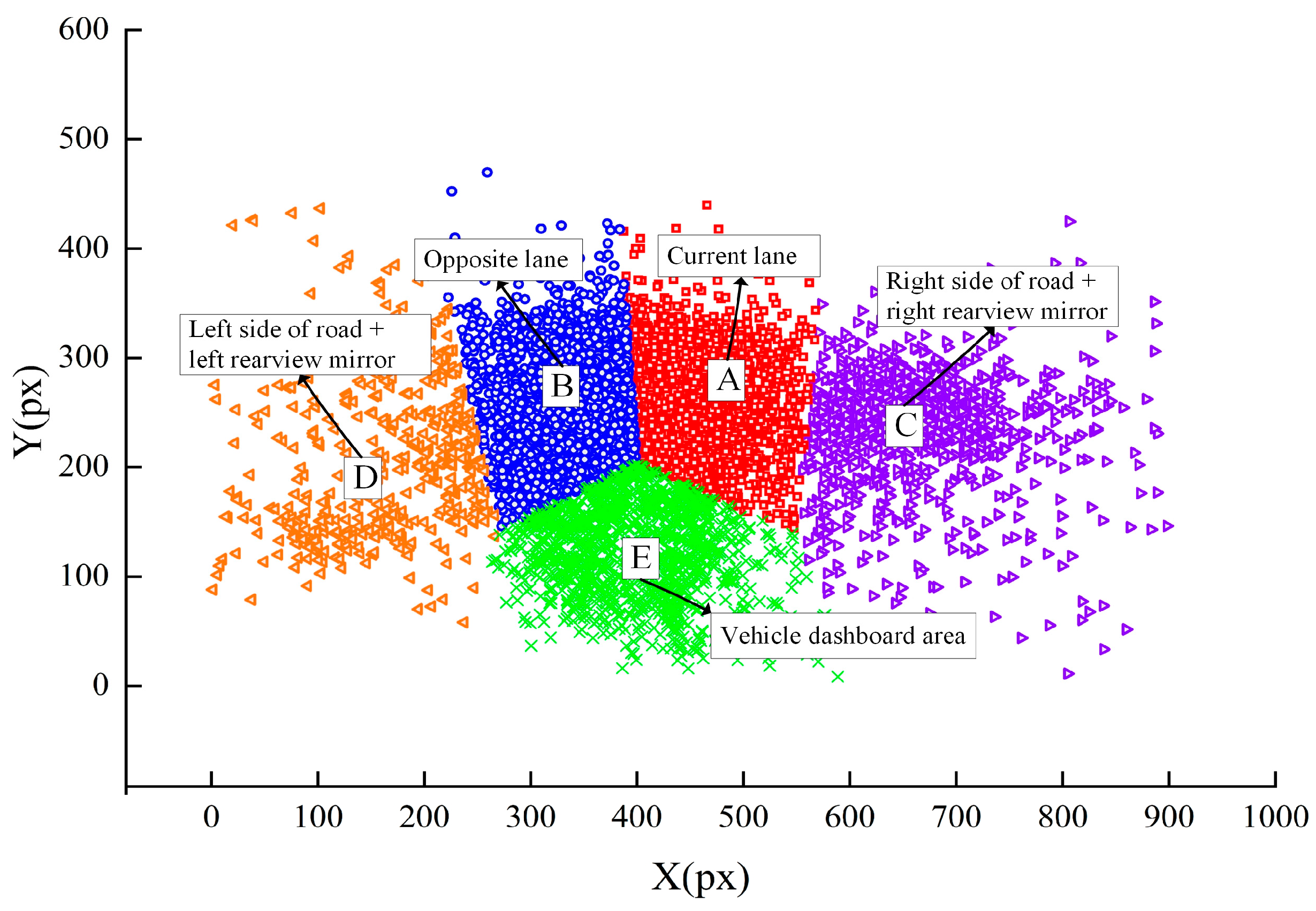
3.1. Cluster Analysis of Fixation Points

Based on the established data time window, we summarized the coordinates of the fixation points from 20 subjects across different traffic environments and subjected these to K-means clustering. The number of clusters was selected as five by combining the study’s objective and the environmental characteristics of the prairie highway, and a combination of the mechanical division method and dynamic clustering method was used to divide the drivers’ visual search area into five parts. Analysis of variance (ANOVA) indicated that the clustering results have significant statistical differences ( p < 0.05 ). The results of the dynamic clustering of fixation point coordinates and visual search area division are shown in Figure 4 and Figure 5. These are as follows: A represents the current driving lane; B is the opposite lane; C is the right side of the road and the right rearview mirror area; D is the left side of the road and the left rearview mirror area; and E is the vehicle dashboard area.
The K-means clustering results are provided in Table 4. During driving, the drivers’ fixation points primarily concentrate in the current lane area, accounting for 47.85% of gaze points, followed by the opposite lane area. The distribution of fixation points on the left side of the road and the left rearview mirror area primarily signifies the drivers’ attention to the connecting section of the left branch at intersections and the left rearview mirror, with the least percentage of fixation points at 4.52%.

3.2. Information Entropy Based on Markov Chain

3.2.1. Analysis of Visual Transfer Modes

The summary number of fixation point transfers of subjects in each traffic environments was greater than 1100 times. Based on the division results of the visual search area, the one-step transition probability of the drivers’ fixation points in different traffic environments was obtained, as shown in Figure 6. Ellipses represent the AOI, with the depth of color representing the probability of drivers’ fixation points transferring to that area. The darker the color, the higher the transition probability. Moreover, the width of the arrow signifies the transition probability between AOIs, with a wider arrow indicating a higher transition probability.
The one-step transition probability of fixation points between AOIs in different traffic environments on prairie highways was analyzed from the perspectives of commonality and variation, as shown in Figure 6.
First, looking at commonality, the one-step transition probability of fixation points in area A is the largest in all six traffic environments. The recurring transition probability within area A is over 60%, suggesting a high level of fixation, which indicates that drivers focus most of their attention on the area in front of the current lane during driving. They tend to keep their gaze fixed in this area to search for and perceive real-time traffic environment information ahead, ensuring smooth vehicle operation across various prairie highway traffic environments.
To analyze variations in drivers’ visual transfer across different traffic environments on prairie highways, we employed the one-step transition probability distribution of drivers’ fixation points during free driving as a control. This allowed us to explore the influence of the five more complex traffic environments on the drivers’ fixation point transfer process. It can be observed from Figure 6 that:
(1)
During vehicle-following, the drivers’ fixation transition probability and recurring fixation probability in area E increase significantly, indicating that drivers need to continually monitor the driving state of the vehicle in front and adjust their speed to maintain a safe following distance. Consequently, they pay more attention to the vehicle’s dashboard, obtaining speed information through multiple repeated fixations (see Figure 6b).
(2)
When encountering an oncoming vehicle, drivers’ fixation transition probability and recurring fixation probability in area B increase significantly. As prairie highways often lack a median strip and traffic control, driving speeds are typically higher than the road design speed. When vehicles approach from the opposite lane, particularly large and medium-sized trucks, drivers divert part of their attention to these oncoming vehicles to maintain a safe lateral distance (see Figure 6c).
(3)
When the rear overtaking vehicles borrow the opposite lane to cut in front of the test vehicle, drivers’ fixation transition probability and recurring fixation probability in areas B and D increase significantly. Drivers must continually monitor the overtaking vehicle’s state from the moment it is observed in the opposite lane or left rearview mirror until it crosses the road centerline and cuts in front of the test vehicle. This is because the safety distance and driving speed of both vehicles mutually restrict each other. Therefore, drivers must continually monitor the overtaking vehicle to adjust their driving strategy and behavior, ensuring safe vehicle operation (see Figure 6d).
(4)
When random risk points appear on the road’s right side, the transition probability and recurring fixation probability significantly increase in area C (where the risk points appear) and area E. Drivers need to continually monitor the dynamic information of risk points and implement certain braking measures to deal with the unpredictable changes in the risk points’ motion states (see Figure 6e).
(5)
When the test vehicle drives straight through an intersection, the distribution of drivers’ fixation points is relatively dispersed, and the fixation transition probability and recurring fixation probability significantly increase in areas C and D. Given that prairie highway intersections prioritize main road traffic, drivers collect traffic information from multiple areas such as the intersection center and the branches on both sides before reaching the intersection. This is done to ensure safe passage through an intersection (see Figure 6f).

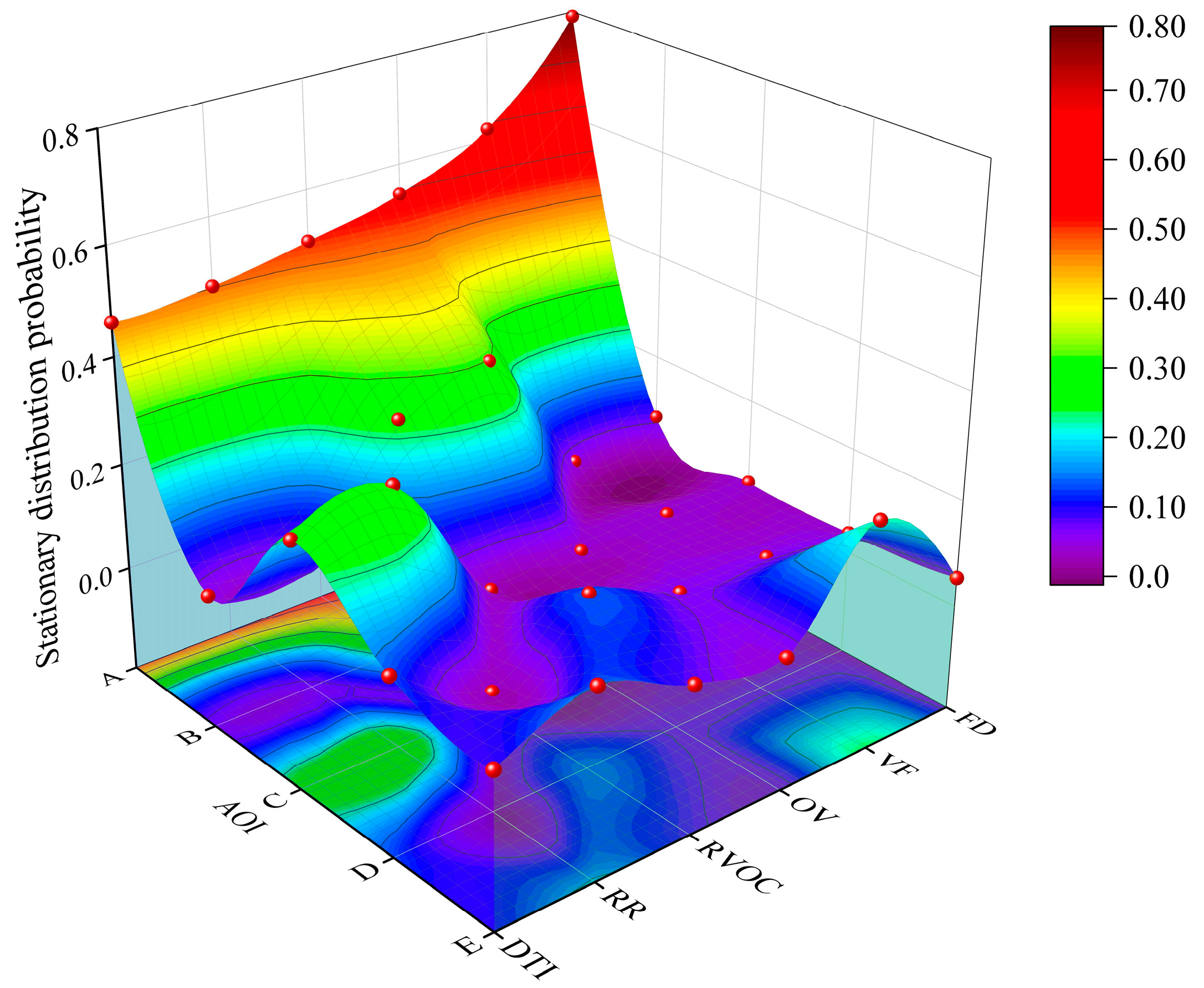
3.2.2. Analysis of Visual Stationary Distribution

The stationary distribution probability of fixation points for each AOI in different traffic environments was calculated (see Figure 7). The stationary distribution probability of drivers’ fixation points in all six traffic environments is the highest in area A, implying that the current driving lane is the primary area where drivers gather traffic environment information. Compared to free driving, the stationary distribution probability of fixation points in area A in the other five relatively complex traffic environments displays varying degrees of decline, with the smallest decrease during vehicle-following (21.64%). The probability in area A significantly drops during driving through intersections and when encountering the roadside risks, with decreases of 40.15% and 41.57%, respectively. This indicates that drivers significantly reduce their focus on the current lane and shift their attention to other areas.
When encountering oncoming vehicles and the rear vehicles overtaking cut-in, drivers must monitor the operational state of vehicles in the opposite lane to maintain a safe lateral distance; thus, the distribution probability of fixation points in area B is higher at 30.69% and 25.49%, respectively. During vehicle movement through roadside risks and intersections, the stationary distribution probability of fixation points in area C significantly increases to 29.21% and 26.18%, respectively. This suggests that drivers shift their focus to the connection section of the right branch of their lane and random risk point locations, respectively, to prepare for risk avoidance behaviors. When driving through intersections and encountering the rear vehicles overtaking cut-in, the distribution probability of fixation points in area D increases significantly (13.11% and 13.22%, respectively), owing to heightened attention in the left rearview mirror and the connection section of the left branch. Additionally, the attention to the vehicle dashboard increases during vehicle-following and navigating through roadside risks, leading to an increase in the stationary distribution probability of fixation points in area E (23.15% and 15.45%, respectively).

3.2.3. Comparative Analysis of Information Entropy of Fixation Distribution (IEFD)

The changes in IEFD of drivers in different traffic environments on prairie roads are shown in Figure 8. Compared to free driving, the IEFD of drivers in the other five relatively complex traffic environments generally increase. The growth rates of average IEFD when vehicle-following and encountering the rear vehicles overtaking cut-in are lower (34.14% and 33.05%, respectively), while the average IEFD significantly increases when encountering oncoming vehicles, roadside risks, and intersections, with growth rates of 58.66%, 62.52%, and 61.02%, respectively. This indicates that increased complexity in the traffic environment prompts drivers to broaden their visual information search area and leads to a more dispersed distribution of fixation points. The variation in IEFD is greater during free driving and encountering the rear vehicles overtaking cut-in. This could be attributed to drivers not needing to focus on a specific AOI during free driving. As a result, their visual search behavior may be influenced by individual visual habits and psychological emotions, leading to a high level of randomness in the transfer path of fixation points. When encountering the rear vehicles overtaking cut-in, individual differences in drivers’ environmental perception and response characteristics lead to variations in the AOI and the time it takes to detect the rear vehicle, resulting in individual variations in fixation point distribution.
One-way repeated measures ANOVA was used to study the significance of differences in drivers’ IEFD in different traffic environments. A Shapiro–Wilk test shows that all groups of data obey normal distribution ( p > 0.05 ), and Mauchly’s sphericity test results show that the sphericity hypothesis is not satisfied ( W = 0.155 , p = 0.005 < 0.05 ); thus, the results were corrected using the Greenhouse–Geisser (GG) method. The analysis results showed that the traffic environments significantly impact drivers’ IEFD ( F = 10.899 , p = 6.855 × 10 6 < 0.05 ). To further analyze the differences in IEFD between free driving and the other five relatively complex driving environments, the Bonferroni correction method was used for pairwise comparisons, as shown in Table 5. The table shows that there are significant differences in IEFD between free driving and the other five traffic environments.

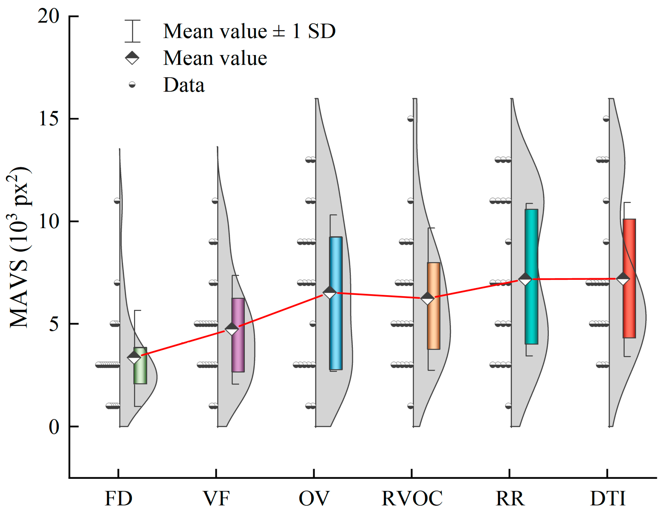
3.3. Comparative Analysis of Main Area of Visual Search (MAVS)

The data of subjects’ fixation points in different traffic environments were counted, and the range of the MAVS in each traffic environment was plotted (see Figure 9). During free driving, fixation points were mainly concentrated in the area in front of the current lane, and the MAVS was approximately circular in distribution. In contrast, the range of MAVS in other relatively complex traffic environments displayed varying degrees of expansion, especially when encountering roadside risks and driving through intersections. This was because drivers paid increased attention to both sides of the road, leading to a more dispersed distribution of fixation points and a significant increase in the range of MAVS.
The MAVS of drivers was segmented into different intervals with a step size of 2000 px2, and the percentage of MAVS in each interval under different traffic environments was calculated (see Figure 10). During free driving, the MAVS was primarily distributed in a small area interval of 1000–3000 px2 with a percentage of 65%. This indicated that the effective visual area where drivers searched for traffic information was smaller, and the attention was more concentrated. However, as the complexity of the traffic environment increased, the percentage of MAVS in the interval of 1000–3000 px2 decreased significantly. Drivers had to expand their visual search range on the road area to ensure driving safety. Notably, when roadside risks appeared, the percentage of MAVS in the large area interval of >9000 px2 was highest, reaching 40%. This showed that the presence of random roadside risks significantly affects the distribution of drivers’ spatial attention and search breadth, leading to a drastic increase in the visual search range.
The MAVS of drivers in different traffic environments was calculated and is shown in Figure 11. In comparison to free driving, the MAVS of drivers in all other five relatively complex traffic environments exhibited an increasing trend. The increase in MAVS during vehicle-following was smaller, and the distribution was similar to that of free driving. This is because, during vehicle-following, drivers primarily focused their visual search area on the vehicle in front, with a smaller part of their attention allocated to the vehicle dashboard area owing to the constraints of the leading vehicle’s speed. The average MAVS of drivers surged when encountering roadside risks and driving through the intersection, both by more than 114% compared to free driving. This indicated that the increased target information on both sides of the road significantly expanded drivers’ visual search range in the horizontal direction, resulting in a larger MAVS.
One-way repeated measures ANOVA was used to study the significance of differences in drivers’ MAVS in different traffic environments. It was tested that all groups of data obey normal distribution ( p > 0.05 ) and satisfy the spherical hypothesis ( W = 0.394 , p = 0.318 > 0.05 ). The analysis results reveal that traffic environments have a significant impact on drivers’ MAVS ( F = 6.584 , p = 2.658 × 10 5 < 0.05 ). The Bonferroni correction method was used for pairwise comparisons, as shown in Table 6. The results indicate that the difference in MAVS between free driving and vehicle-following is not statistically significant, whereas significant differences exist with all four other traffic environments.

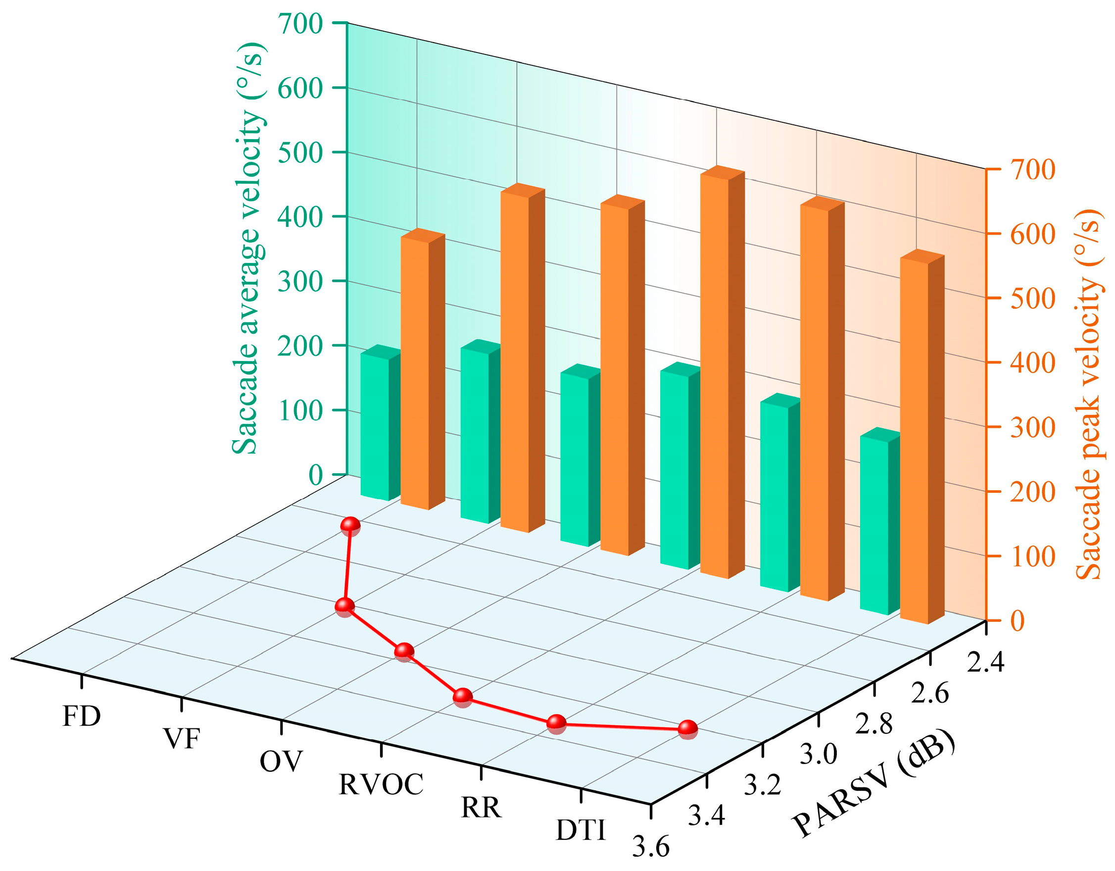
3.4. Comparative Analysis of Peak-to-Average Ratio of Saccade Velocity (PARSV)

The PARSV of drivers in different traffic environments was calculated and is shown in Figure 12. The average PARSV is lowest during free driving. This is because the driving environment is relatively comfortable and safe, enabling drivers to not frequently search the surrounding environment for information. This results in lower environmental perception and alertness, and higher visual stability. However, the average PARSV increases sharply compared with free driving when encountering rear vehicles overtaking cut-in and roadside risks during driving, with growth rates of 25.41% and 26.25%, respectively. This shows that the appearance of rear overtaking vehicles and random roadside risks creates a strong visual stimulus for drivers, which makes drivers’ alertness rise rapidly. This leads to significant fluctuations in saccade velocity and decreased visual stability.
After testing, all groups of data obey normal distribution ( p > 0.05 ) and satisfy the spherical hypothesis ( W = 0.263 , p = 0.063 > 0.05 ). One-way repeated measures ANOVA shows that traffic environments significantly impact drivers’ PARSV ( F = 8.406 , p = 1.294 × 10 6 < 0.05 ). The Bonferroni correction method was used for pairwise comparisons, as shown in Table 7. The results indicate that the difference in PARSV between free driving and vehicle-following is marginally significant ( p < 0.1 ), whereas significant differences exist within all four other traffic environments.
Figure 13 presents the variations in saccade average velocity, saccade peak velocity, and PARSV for drivers across different traffic conditions on prairie highways. The analysis reveals that while the change rules of these three indicators do not perfectly align, they share some common trends. Both saccade average velocity and saccade peak velocity dip to their lowest values during free driving, and they tend to rise with the increased complexity of the traffic environment. A noticeable surge occurs when drivers encounter rear vehicles overtaking cut-in and roadside risks. This change rule is consistent with the PARSV analysis, indicating that an acceleration in saccade velocity often results in decreased visual stability. These observations further affirm the validity of the PARSV analysis results.

3.5. Evaluation of Driving Safety Based on Visual Search Load

A driver’s visual search load comprehensively characterizes the visual resources consumed in searching for information in the traffic environment, which affects the driver’s visual information processing ability and is an essential factor affecting driving safety. In this study, three indicators—IEFD, MAVS, and PARSV—were chosen from the driver’s visual search level to construct an evaluation system. Mathematical and statistical methods were used to analyze the differential change of each indicator under various traffic environments. These chosen indicators aim to explore the visual resources that drivers use to gather environmental information in different traffic situations and to analyze changes in driving safety from a visual search load perspective. To gauge the relative importance of each visual search indicator within the evaluation system, the improved CRITIC method was initially used to assign weights to the indicators objectively. The variation coefficient of each indicator and the correlation coefficient between them were calculated, providing a comprehensive measure of the information each indicator contains and determining their weights. The results of these calculations are shown in Table 8.
Based on the constructed visual search indicators and their weight system, the VIKOR method was used to consider the drivers’ visual search load level in terms of visual search complexity, stability, and visual field range and to further conduct a comprehensive evaluation of driving safety. By analyzing the indicator characteristics, the positive and negative ideal solutions were defined as the minimum and maximum values of each visual search indicator, respectively, and the positive ideal solution measured an idealized traffic environment with the lowest visual search load. Taking the positive and negative ideal solutions as a reference, the group utility value S i and individual regret value R i of each traffic environment were calculated to characterize its proximity to the idealized traffic environment. Finally, the synthesis decision-making value Q i was calculated by considering group utility and individual regret and combining decision preferences. Among them, the group utility value S i takes the overall change characteristics of visual search behavior as a measure and reflects the comprehensive influence effect of traffic environment on visual search load based on multi-featured indicators, while individual regret value R i only reflects the prominent influence effect of traffic environment on visual search behavior in terms of a certain characteristic.
First, the decision-making mechanism coefficient μ was selected at 0.5 to make a compromise decision-making [50,51,52]. The S i , R i , and Q i values of six traffic environments were calculated, respectively, and the traffic environments were ranked in ascending order according to the Q i values. The results of the VIKOR analysis are shown in Table 9. Analysis of Table 9 shows that Q ( f 2 ) Q ( f 1 ) = 0.522 1 / 5 , which satisfies Criterion 1, and that both S h and R h rank first when driving freely, which satisfies Criterion 2. Therefore, the six traffic environments were ranked in ascending order of the Q i value as follows: FD < VF < RVOC < OV < DTI < RR. The Q i value of free driving was the minimum, indicating that the drivers’ visual search load is the lowest and driving safety is relatively high. The Q i value surged when the traffic environment presented roadside risks, indicating that the emergence of random roadside risks significantly affects drivers’ visual search behavior, resulting in the highest visual search load and the lowest driving safety, followed by intersections.
The value of the decision-making mechanism coefficient μ in the VIKOR method indicates the difference in decision-making tendency for group utility and individual regret, with the possibility of the μ value affecting the final decision-making result [51,52]. To analyze the influence of different decision-making tendencies on the ranking results of the traffic environment, different values of μ between zero and one were used for sensitivity analysis. The calculated results of Q i values under different μ value conditions are shown in Figure 14, and the ranking under each μ value condition passed the criterion validation. Figure 14 shows that the ranking of traffic environment is the same under different μ value conditions, indicating that the evaluation results of visual search load are not sensitive to the decision-making mechanism coefficient μ and have better decision-making stability.

4. Discussion

Drivers’ visual search behavior directly influences their perception and acquisition of traffic environment information, thereby playing a crucial role in driving safety. The goal of this study was to analyze the specific visual search strategies employed by drivers in diverse traffic environments on prairie highways. We aimed to introduce the concept of visual search load to evaluate driving safety from a human-factor security perspective.
In this study, we employed the K-means clustering method to segment the drivers’ visual search area into five AOIs. We then utilized the Markov chain model to predict and analyze the transfer and stationary distribution characteristics of the drivers’ fixation points within each AOI under varying traffic environments. This reflected the flow and distribution of attention in space [18,59]. Our findings affirmed the hypothesis that the type of traffic environment significantly influences drivers’ patterns of visual distribution and transfer. Within the six traffic environments identified on the prairie highway, the transition probability and stationary distribution probability of the drivers’ fixation points were greatest in the current lane area. The recurring transition probability within this area exceeded 60%, suggesting that the current lane is the main search area for collecting traffic environment information. Qin et al. [17] studied drivers’ visual differences on each typical road section of a mountainous low-grade highway using Markov chains and found that the stationary fixation probability of drivers looking ahead in different road sections surpassed 70%. This concentration of fixation points at the front assists drivers more effectively in observing the road traffic situation, a finding that aligns with our own results. We also found that, compared to free driving, the attention devoted to the current lane in five other relatively complex traffic environments significantly decreased as the drivers’ attention distribution area increased. This was particularly noticeable when driving through the intersection and encountering roadside risks, where the stationary distribution probability of fixation points in the current lane area dropped sharply, decreasing by 40.15% and 41.57%, respectively. Similar conclusions were reached in the study by Li et al. [60]. In stressful scenarios involving a moving target, drivers typically select one or two auxiliary areas to supplement their information acquisition based on the target’s range of motion.
Subsequently, we incorporated the Markov chain theory into our information entropy study, constructing the IEFD indicator to quantify the complexity of drivers’ search for traffic information across the entire visual field. Concurrently, we introduced the MAVS indicator to express the breadth and spatial concentration of the drivers’ attention within the visual field. We also established the PARSV indicator to represent the dynamic equilibrium degree of visual search behavior. Mathematical statistics revealed statistically significant differences in the visual evaluation indicators as the traffic environment varied. The IEFD and MAVS were highest when drivers encountered intersection and roadside risks, with drivers focused on the road ahead and the branches on both sides when driving through intersections, and the presence of random roadside risk points similarly attracted their attention to roadside areas. This confirms the hypothesis that the increase in environmental elements along the roadside heightens the difficulty of visual information acquisition while broadening the driver’s visual search range. Wang et al. [50] were the first to define PARSV to compare the differences in visual stability between normal and distracted driving states. Their research discovered that drivers’ visual stability tended to decrease when they were distracted by operating a cell phone. The visual secondary task occupied some of the drivers’ attention resources, leading to a surge in drivers’ PARSV and a significant decrease in visual stability. In our research, we found the PARSV to be lowest during free driving, with the driver’s visual information processing intensity being lower and visual stability higher owing to the relatively monotonous driving environment. Conversely, the PARSV of drivers in the other five relatively complex traffic environments generally increased, with a surge in PARSV when encountering rear vehicles overtaking cut-in and roadside risks. This increase followed the same trend as the saccade speed. This confirms the hypothesis that an increase in traffic environment information accelerates the driver’s visual search behavior and often coincides with a decrease in visual stability.
Based on the objective weighting of the indicators by the improved CRITIC method, we used the VIKOR method to comprehensively evaluate drivers’ visual search load in different traffic environments. The ascending order of visual search load for the six driving environments is as follows: FD < VF < RVOC < OV < DTI < RR. During free driving, the drivers’ visual search load is the lowest, and driving safety is relatively high. In contrast, the presence of roadside risks significantly impacts drivers’ visual search behavior, and drivers experience the greatest visual search load, resulting in significantly reduced driving safety. Considering that the evaluation results may be affected by the decision-making tendency, we made further sensitivity analysis of the results and verified that the driving safety evaluation based on the visual search load has better decision-making stability.
Despite the insightful findings, there are several limitations to this research that need acknowledgment, as they will help guide future research directions.
  • Since the site of the real vehicle test was located in a vast prairie area far from urban areas, the implementation of the test was limited by safety, cost, and time, so the sample size for completing the test was not sufficient, and the data collection process cannot accurately control the consistency of the test conditions, and the test results may have certain errors. Future research can increase the test scenarios in combination with simulated driving and carry out a total-factor analysis by taking into account individual attribute characteristics such as the driver’s gender and driving experience on the basis of expanding the sample size;
  • The collection of drivers’ eye movement data in the test was based on a head-mounted eye tracker. Although the instrument has a high measurement accuracy, long-term wearing may cause fatigue and discomfort to the drivers. Therefore, the next step could be equipped with a remote eye tracker (RED) to improve our study. The RED installed in the vehicle will improve the driving safety during the test and bring the driving behavior closer to the real state;
  • In this study, the analysis of driving safety only considered the driver’s visual behavioral characteristics, but the recognition effect of different types of indicators on driving safety may be different. Future research can increase the evaluation indicators of psychology, operation reaction, and other aspects, deeply analyze the applicable scenarios and sensitivity of the indicators, and combine the multi-featured parameters to comprehensively analyze driving safety to improve the scientific validity of the research.

5. Conclusions

Considering the paucity of in-depth analyses of drivers’ visual search behavior in varying traffic environments on prairie highways in prior studies, this research designed and carried out a real vehicle test on prairie highways. It collected eye movement data of drivers across six real traffic environments, compared the differences in drivers’ visual search behavior across these environments, and evaluated the driving safety level from a visual search perspective. Based on the results, the following conclusions can be drawn:
(1)
The distribution and transfer of drivers’ visual attention differ according to the traffic environments on prairie highways. However, the current lane consistently remains the main search area for drivers to obtain traffic information. During free driving, drivers primarily focus on the current lane area, and their visual attention is highly concentrated. In contrast, as the components elements of the traffic environment increase, drivers tend to shift their attention to multiple AOIs to supplement information acquisition. The selection of AOIs largely depends on the location and motion state of the target that affects driving safety, which reduces attention to the current lane.
(2)
IEFD, PARSV, and MAVS analyze drivers’ visual search characteristics in terms of visual search complexity, stability, and visual field range, respectively. Mathematical statistics results show that these visual evaluation indicators demonstrate significant statistical differences with changes in the driving environment. Evidently, increased information about the traffic environment prompts drivers to expand their main visual search area, thereby increasing the complexity of visual information processing and decreasing visual stability.
(3)
The concept of visual search load was introduced for a comprehensive evaluation of driving safety. The analysis showed that drivers’ visual search load is the lowest during free driving, resulting in relatively high driving safety. In contrast, the emergence of roadside risks considerably affects drivers’ visual search behavior, leading to increased visual search load and significantly reduced driving safety. Sensitivity analysis verifies that the evaluation results of visual search load are not affected by decision-making tendency and exhibit robust decision-making stability. Hence, the roadside environment is a critical factor affecting driving safety on prairie highways. To improve driving safety on these highways, attention should be focused on assessing roadside safety hazards and targeting the construction of safety facilities and traffic management.
This research contributes to the improvement of the evaluation indicator system and analysis methods of visual search behavior. It holds considerable theoretical value for targeted correction of undesirable visual search behavior on prairie highways and further exploration of driving safety hazards and accident causation on these highways. Moreover, the traffic safety evaluation model based on the VIKOR method provides a new avenue for research on traffic human safety. The design of real vehicle tests and the selection of traffic environments can serve as a reference for similar studies. The research findings can guide driving behavior intervention and graded early warning, the enhancement of traffic safety facilities on prairie highways, and improvement of traffic management.

Author Contributions

Conceptualization, X.D. and H.W.; methodology, X.D.; software, C.W.; validation, H.W. and M.G.; formal analysis, X.D.; investigation, X.D. and C.W.; data curation, H.W.; writing—original draft preparation, X.D.; writing—review and editing, X.D. and H.W.; supervision, H.W.; project administration, H.W. and M.G.; funding acquisition, H.W. All authors have read and agreed to the published version of the manuscript.

Funding

This research was funded by the Inner Mongolia Autonomous Region Science and Technology Plan Project (grant number: 2022YFSH0071), the Program for Innovative Research Team in Universities of Inner Mongolia Autonomous Region (grant number: NMGIRT2304), and the Higher Education Science and Technology Research Project of Inner Mongolia Autonomous Region (grant number: NJZY23112).

Institutional Review Board Statement

This study was submitted to the Ethics Committee of Inner Mongolia Agricultural University on 16 May 2022, and ethical review and approval were exempted because the data collection posed no more than minimal risk to participants and would not cause any mental injury to the participants, have any negative social impact, or influence the participants’ subsequent behavior. Any risks during the experiment were informed, and participants were allowed to leave whenever they felt uncomfortable.

Informed Consent Statement

Informed consent was obtained from all subjects involved in the study.

Data Availability Statement

The data supporting the findings of this study are available from the corresponding author upon reasonable request.

Conflicts of Interest

The authors declare no conflict of interest.

References

  1. Kumeda, B.; Zhang, F.; Alwan, G.M.; Owusu, F.; Hussain, S. A hybrid optimization framework for road traffic accident data. Int. J. Crashworthiness 2021, 26, 246–257. [Google Scholar] [CrossRef]
  2. Cheng, Y.; Gao, L.; Zhao, Y.; Du, F. Drivers’ visual characteristics when merging onto or exiting an urban expressway. PLoS ONE 2016, 11, e0162298. [Google Scholar] [CrossRef] [PubMed] [Green Version]
  3. Farooq, D.; Moslem, S.; Duleba, S. Evaluation of driver behavior criteria for evolution of sustainable traffic safety. Sustainability 2019, 11, 3142. [Google Scholar] [CrossRef] [Green Version]
  4. Baldo, N.; Marini, A.; Miani, M. Drivers’ braking behavior affected by cognitive distractions: An experimental investigation with a virtual car simulator. Behav. Sci. 2020, 10, 150. [Google Scholar] [CrossRef] [PubMed]
  5. Wang, X. Traffic Safety Analyses; Tongji University Press: Shanghai, China, 2022; pp. 1–26. [Google Scholar]
  6. Kircher, K.; Ahlstrom, C. Minimum required attention: A human-centered approach to driver inattention. Hum. Factors 2017, 59, 471–484. [Google Scholar] [CrossRef]
  7. Liu, C.; Wang, Z.; Nacpil, E.J.C.; Hou, W.; Zheng, R. Analysis of visual risk perception model for braking control behaviour of human drivers: A literature review. IET Intell. Transp. Syst. 2022, 16, 711–724. [Google Scholar] [CrossRef]
  8. Zhang, D.; Chen, F.; Zhu, J.; Wang, C.; Cheng, J.; Zhang, Y.; Bo, W.; Zhang, P. Research on drivers’ hazard perception in plateau environment based on visual characteristics. Accid. Anal. Prev. 2022, 166, 106540. [Google Scholar] [CrossRef]
  9. Konstantopoulos, P.; Crundall, D. The driver prioritisation questionnaire: Exploring drivers’ self-report visual priorities in a range of driving scenarios. Accid. Anal. Prev. 2008, 40, 1925–1936. [Google Scholar] [CrossRef] [PubMed]
  10. Zhang, W.; Dai, J.; Pei, Y.; Li, P.; Yan, Y.; Chen, X. Drivers’ visual search patterns during overtaking maneuvers on freeway. Int. J. Environ. Res. Public Health 2016, 13, 1159. [Google Scholar] [CrossRef] [Green Version]
  11. Dukic, T.; Broberg, T. Older drivers’ visual search behaviour at intersections. Transp. Res. Part F Traffic Psychol. Behav. 2012, 15, 462–470. [Google Scholar] [CrossRef]
  12. Ponnambalam, C.T.; Donmez, B. Searching for street parking: Effects on driver vehicle control, workload, physiology, and glances. Front. Psychol. 2020, 11, 574262. [Google Scholar] [CrossRef]
  13. Crundall, D.; Shenton, C.; Underwood, G. Eye movements during intentional car following. Perception 2004, 33, 975–986. [Google Scholar] [CrossRef]
  14. Sun, Q.C.; Xia, J.C.; He, J.B.; Foster, J.; Falkmer, T.; Lee, H. Towards unpacking older drivers’ visual-motor coordination: A gaze-based integrated driving assessment. Accid. Anal. Prev. 2018, 113, 85–96. [Google Scholar] [CrossRef]
  15. Stahl, P.; Donmez, B.; Jamieson, G.A. Eye glances towards conflict-relevant cues: The roles of anticipatory competence and driver experience. Accid. Anal. Prev. 2019, 132, 105255. [Google Scholar] [CrossRef] [PubMed]
  16. Lemonnier, S.; Desire, L.; Bremond, R.; Baccino, T. Drivers’ visual attention: A field study at intersections. Transp. Res. Part F Traffic Psychol. Behav. 2020, 69, 206–221. [Google Scholar] [CrossRef]
  17. Qin, Y.; Yang, N.; Xie, J.; Zhao, S.; Qian, Z. Analysis of drive’s visual differences in typical sections of low-grade highways in mountainous areas. J. Saf. Environ. 2022, 22, 3235–3243. [Google Scholar]
  18. Li, G.; Wang, Y.; Zhu, F.; Sui, X.; Wang, N.; Qu, X.; Green, P. Drivers’ visual scanning behavior at signalized and unsignalized intersections: A naturalistic driving study in China. J. Saf. Res. 2019, 71, 219–229. [Google Scholar] [CrossRef]
  19. Wu, F.; Fu, R.; Wang, X.; Liu, J. Influence of cut-in situation on driving behavior of the following car drivers. Lect. Notes Electr. Eng. 2020, 576, 653–660. [Google Scholar]
  20. Yuan, W.; Fu, R.; Guo, Y.; Wu, F. Analysis on drivers’ dynamic visual characters in different road conditions. In Proceedings of the International Conference on Communication and Vehicular Technology (ICCVT), Hanoi, Vietnam, 30–31 December 2010. [Google Scholar]
  21. Chung, J.; Lee, H.; Moon, H.; Lee, E. The static and dynamic analyses of drivers’ gaze movement using VR driving simulator. Appl. Sci. 2022, 12, 2362. [Google Scholar] [CrossRef]
  22. Du, J.; Ren, G.; Liu, W.; Li, H. How is the visual working memory load of driver influenced by information density of traffic signs? Transp. Res. Part F Traffic Psychol. Behav. 2022, 86, 65–83. [Google Scholar] [CrossRef]
  23. Hu, J.B.; Wang, R.H. Classification of driving workload affected by highway alignment conditions based on classification and regression tree algorithm. Traffic Inj. Prev. 2018, 19, 214–218. [Google Scholar] [CrossRef] [PubMed]
  24. Ringhand, M.; Siebke, C.; Baumler, M.; Petzoldt, T. Approaching intersections: Gaze behavior of drivers depending on traffic, intersection type, driving maneuver, and secondary task involvement. Transp. Res. Part F Traffic Psychol. Behav. 2022, 91, 116–135. [Google Scholar] [CrossRef]
  25. Miller, K.A.; Chapman, P.; Sheppard, E. A cross-cultural comparison of where drivers choose to look when viewing driving scenes. Transp. Res. Part F Traffic Psychol. Behav. 2021, 81, 639–649. [Google Scholar] [CrossRef]
  26. Lyu, Z.; Qi, C.; Zhu, S. Driver’s attention allocation and mental workload at different random hazard points on prairie highway. J. Adv. Transp. 2022, 2022, 3837509. [Google Scholar] [CrossRef]
  27. Zhang, Y.; Zhu, S. Study on the effect of driving time on fatigue of grassland road based on EEG. J. Healthc. Eng. 2021, 2021, 1–9. [Google Scholar] [CrossRef]
  28. Li, H.; Xie, S.; Yang, F.; Lu, Y.; Zhu, S. Utilization of drivers’ dynamic visual characteristics to find the appropriate information quantity of traffic engineering facilities on straight roads of grassland highways. Front. Neurosci. 2022, 16, 3837509. [Google Scholar] [CrossRef] [PubMed]
  29. Peng, Z.; Rong, J.; Wu, Y.; Zhou, C.; Yuan, Y.; Shao, X. Exploring the different patterns for generation process of driving fatigue based on individual driving behavior parameters. Transp. Res. Rec. 2021, 2675, 408–421. [Google Scholar] [CrossRef]
  30. Liu, Y.; Zhao, X.; Wu, Y. Study on the effectiveness of driving fatigue prevention safety facility on grassland highway based on driving simulation. In Proceedings of the ASCE International Conference on Transportation and Development (ASCE ICTD), Seattle, WA, USA, 26–29 May 2020; pp. 264–274. [Google Scholar]
  31. Li, X.; Han, L.; Zhu, S.; Gao, M. Information quantity of traffic signs in grassland highways based on visual load. J. Comput. Methods Sci. Eng. 2021, 21, 2077–2091. [Google Scholar] [CrossRef]
  32. Wang, F.; Li, X.; Guo, H.; Hu, J. Optimization of straight segment index between highway curves of desert grassland based on driver’s visual interest region. J. Jilin Univ. 2020, 50, 114–120. [Google Scholar]
  33. Wu, Y.B.; Kihara, K.; Takeda, Y.; Sato, T.; Akamatsu, M.; Kitazaki, S.; Nakagawa, K.; Yamada, K.; Oka, H.; Kameyama, S. Eye movements predict driver reaction time to takeover request in automated driving: A real-vehicle study. Transp. Res. Part F Traffic Psychol. Behav. 2021, 81, 355–363. [Google Scholar] [CrossRef]
  34. Gemonet, E.; Bougard, C.; Masfrand, S.; Honnet, V.; Mestre, D.R. Car drivers coping with hazardous events in real versus simulated situations: Declarative, behavioral and physiological data used to assess drivers’ feeling of presence. PLoS ONE 2021, 16, e0247373. [Google Scholar] [CrossRef]
  35. Dowiasch, S.; Wolf, P.; Bremmer, F. Quantitative comparison of a mobile and a stationary video-based eye-tracker. Behav. Res. Methods 2020, 52, 667–680. [Google Scholar] [CrossRef]
  36. Qin, L.; Shi, Y.; He, Y.; Zhang, J.; Zhang, X.; Li, Y.; Deng, T.; Yan, H. ID-YOLO: Real-time salient object detection based on the driver’s fixation region. IEEE Trans. Intell. Transp. Syst. 2022, 23, 15898–15908. [Google Scholar] [CrossRef]
  37. Greenberg, A.S.; Rosen, M.; Cutrone, E.; Behrmann, M. The effects of visual search efficiency on object-based attention. Atten. Percept. Psychophys. 2015, 77, 1544–1557. [Google Scholar] [CrossRef] [PubMed]
  38. Li, S.; Ji, B.; Sun, W.; Wang, L.; Yang, Z. Study on the influence of driving experience on visual characteristic. Adv. Mech. Eng. 2013, 2013, 790813. [Google Scholar] [CrossRef] [Green Version]
  39. Xu, Q.; Guo, T.; Shao, F.; Jiang, X. Division of area of fixation interest for real vehicle driving tests. Math. Probl. Eng. 2017, 2017, 3674374. [Google Scholar] [CrossRef] [Green Version]
  40. Shang, T.; Qi, H.; Huang, A.; Liu, T. A comparative driving safety study of mountainous expressway individual tunnel and tunnel group based on eye gaze behavior. PLoS ONE 2022, 17, e0263835. [Google Scholar] [CrossRef] [PubMed]
  41. Peng, J.S.; Wang, C.W.; Fu, R.; Yuan, W. Extraction of parameters for lane change intention based on driver’s gaze transfer characteristics. Saf. Sci. 2020, 126, 104647. [Google Scholar] [CrossRef]
  42. Blazejczyk, P.; Magdziarz, M. Stochastic modeling of Levy-like human eye movements. Chaos 2021, 31, 104647. [Google Scholar] [CrossRef]
  43. Shang, T.; Lu, H.; Wu, P.; Lu, X. Method of setting exit advance guide signs in highway tunnels based on the driver’s eye movement with markov chains. IEEE Access 2021, 9, 24079–24092. [Google Scholar] [CrossRef]
  44. Sammaknejad, N.; Pouretemad, H.; Eslahchi, C.; Salahirad, A.; Alinejad, A. Gender classification based on eye movements: A processing effect during passive face viewing. Adv. Cogn. Psychol. 2017, 13, 232–240. [Google Scholar] [CrossRef] [Green Version]
  45. Wang, Y.; Wang, L.; Lin, S.; Cong, W.; Xue, J.; Ochieng, W. Effect of working experience on air traffic controller eye movement. Engineering 2021, 7, 488–494. [Google Scholar] [CrossRef]
  46. Roy, S. Quantifying interactions among car drivers using information theory. Chaos 2020, 30, 104647. [Google Scholar] [CrossRef]
  47. Miura, A.; Tomoeda, A.; Nishinari, K. Formularization of entropy and anticipation of metastable states using mutual information in one-dimensional traffic flow. Physica A 2020, 560, 125152. [Google Scholar] [CrossRef]
  48. Wang, S.; Du, Z.; Feng, S.; Jiao, F.; Xu, F. Research on effectiveness of visual guiding system in entrance zone of freeway tunnel. J. Traffic Transp. Eng. 2021, 21, 267–277. [Google Scholar]
  49. Yang, J.; Liu, C.; Chu, P.; Wen, X.; Zhang, Y. Exploration of the relationships between hazard perception and eye movement for young drivers. J. Adv. Transp. 2021, 2021, 6642999. [Google Scholar] [CrossRef]
  50. Wang, H.; Ding, X.; Wang, C. Risk assessment of distracted driving behavior based on visual stability coefficient. J. Adv. Transp. 2023, 2023, 2111532. [Google Scholar] [CrossRef]
  51. Ali, J. A novel score function based CRITIC-MARCOS method with spherical fuzzy information. Comput. Appl. Math. 2021, 40, 280. [Google Scholar] [CrossRef]
  52. Mishra, A.R.; Bullet, P.R.; Pandey, K. Fermatean fuzzy CRITIC-EDAS approach for the selection of sustainable third-party reverse logistics providers using improved generalized score function. J. Ambient Intell. Humaniz. Comput. 2022, 13, 295–311. [Google Scholar] [CrossRef]
  53. Torkayesh, A.E.; Ecer, F.; Pamucar, D.; Karamasa, C. Comparative assessment of social sustainability performance: Integrated data-driven weighting system and CoCoSo model. Sustain. Cities Soc. 2021, 71, 102975. [Google Scholar] [CrossRef]
  54. Liu, X.; Wang, Z.; Zhang, S.; Chen, Y. Investment decision making along the B&R using CRITIC approach in probabilistic hesitant fuzzy environmen. J. Bus. Econ. Manag. 2020, 21, 1683–1706. [Google Scholar]
  55. Xu, F.; Liu, J.; Lin, S.; Yuan, J. A VIKOR-based approach for assessing the service performance of electric vehicle sharing programs: A case study in Beijing. J. Clean Prod. 2017, 148, 254–267. [Google Scholar] [CrossRef]
  56. Katanalp, B.Y.; Eren, E.; Alver, Y. An integrated solution to identify pedestrian-vehicle accident prone locations: GIS-based multicriteria decision approach. J. Transp. Saf. Secur. 2023, 15, 137–176. [Google Scholar] [CrossRef]
  57. Alemdar, K.D.; Kaya, O.; Codur, M.Y. A GIS and microsimulation-based MCDA approach for evaluation of pedestrian crossings. Accid. Anal. Prev. 2020, 148, 102975. [Google Scholar] [CrossRef]
  58. Drissi, M.; Oumsis, M.; Aboutajdine, D. A multi-criteria decision framework for network selection over LTE and WLAN. Eng. Appl. Artif. Intell. 2017, 66, 113–127. [Google Scholar] [CrossRef]
  59. Munoz, M.; Reimer, B.; Lee, J.; Mehler, B.; Fridman, L. Distinguishing patterns in drivers’ visual attention allocation using Hidden Markov Models. Transp. Res. Part F Traffic Psychol. Behav. 2016, 43, 90–103. [Google Scholar] [CrossRef]
  60. Li, X.; Meng, F.; Zheng, X.; Ren, Y.; Yan, J. Driver’s visual characterization based on stress response. J. Jilin Univ. 2017, 47, 1403–1410. [Google Scholar]
Figure 1. Test road environment. The red cross mark represents the position of the driver’s fixation point.
Sustainability 15 12146 g001
Figure 2. Main test equipment.
Sustainability 15 12146 g002
Figure 3. Schematic of traffic environments. (a) FD; (b) VF; (c) OV; (d) RVOC; (e) RR; (f) DTI. The arrows indicate the direction of vehicles driving.
Sustainability 15 12146 g003aSustainability 15 12146 g003b
Figure 4. Dynamic clustering results of fixation points.
Sustainability 15 12146 g004
Figure 5. Division of driver’s visual search area. The red cross mark represents the position of the driver’s fixation point.
Sustainability 15 12146 g005
Figure 6. One-step transition probability diagram of fixation points in different traffic environments. (a) FD; (b) VF; (c) OV; (d) RVOC; (e) RR; (f) DTI. A–E denotes different AOIs.
Sustainability 15 12146 g006aSustainability 15 12146 g006b
Figure 7. Stationary distribution probability of fixation points. The red dots indicate the stationary distribution probability of fixation points for each AOI in different traffic environments.
Sustainability 15 12146 g007
Figure 8. Comparison of IEFD in different traffic environments. The shadow shows the distribution of the data and its probability density.
Sustainability 15 12146 g008
Figure 9. Visual main search area in different traffic environments. (a) FD; (b) VF; (c) OV; (d) RVOC; (e) RR; (f) DTI.
Sustainability 15 12146 g009aSustainability 15 12146 g009b
Figure 10. Percentage of MAVS in each interval under different traffic environments.
Sustainability 15 12146 g010
Figure 11. Comparison of MAVS in different traffic environments. The shadow shows the distribution of the data and its probability density.
Sustainability 15 12146 g011
Figure 12. Comparison of PARSV in different traffic environments. The shadow shows the distribution of the data and its probability density.
Sustainability 15 12146 g012
Figure 13. Changes in saccade velocity and PARSV in different traffic environments.
Sustainability 15 12146 g013
Figure 14. Influence of μ on traffic environment ranking results.
Sustainability 15 12146 g014
Table 1. Road and traffic parameters of the test road section.
Road and Traffic ParametersValue or Characteristic
Road length (km)150
Road speed limit (km/h)80
Number of two-way lanes (lines) and width (m)2/3.5
Hard shoulder width (m)1
Ratio of straight-line segment (%)80
Pavement typeAsphalt pavement
Intersection control methodMain road priority control
Table 2. Basic parameters of Iview X HED.
Technical ParametersParameter Value
ModelIview X HED
Sampling frequency (Hz)200
Tracking resolution (°)0.1
Fixation positioning accuracy (°)0.5–1
Tracking angle (°)Horizontal angle: +/−30
Vertical angle: +/−25
Table 3. Interpretation and data windows of different traffic environments.
Traffic EnvironmentDefinitionData Window
Free driving
(FD)
During driving, the field of view is free of other traffic participants, roadside risks, intersections, and related safety facilities.Combined with the test process and data fluctuations, the data window for vehicle-following and free driving is 20 s.
Vehicle-following
(VF)
Since the test vehicle cannot overtake the vehicles traveling in the same lane, maintaining a safe following distance is necessary.
Oncoming vehicles
(OV)
Vehicles are approaching from the opposite lane.Starts when the subject’s fixation point falls on the vehicle in the opposite lane for the first time until the meeting is completed.
Rear vehicles overtaking cut-in
(RVOC)
The rear vehicles in the same lane overtake and cut in front of the test vehicle.Starts when the subject first detects the rear lane-changing vehicles from the left rearview mirror or the opposite lane until they cross the road centerline and cut in front of the test vehicle.
Roadside risks
(RR)
Random roadside risks of prairie highways include animals, parked vehicles, pedestrians, etc.Starts when the subject’s fixation point falls on the random risk points on the right side of the driving lane for the first time until the test vehicle passes.
Driving through intersections
(DTI)
The test vehicle proceeds straight through intersections.We noted that subjects typically began seeking traffic information when they were approximately 8 seconds’ driving distance from the intersection. Consequently, we focused our study on the 8 s period before the test vehicle crossed the intersection.
Table 4. Clustering center and percentage of attention points results.
CategoryClustering AreaClustering CenterPercentage of Fixation Points (%)
ACurrent lane(453.58, 257.46)47.85
BOpposite lane(339.21, 249.17)22.03
CRight side of road and right rearview mirror(666.58, 236.34)14.09
DLeft side of road and left rearview mirror area(161.34, 208.17)4.52
EVehicle dashboard area(397.83, 126.34)11.50
Table 5. Pairwise comparison results of IEFD for different traffic environments.
IndicatorComparison of Traffic Environment | t |   Value p Value
IEFDFDVF3.2720.022
OV5.6232.814 × 10−6
RVOC3.1680.031
RR5.9935.527 × 10−7
DTI5.8491.047 × 10−6
Note: p < 0.05 indicates a significant difference.
Table 6. Pairwise comparison results of MAVS for different traffic environments.
IndicatorComparison of Traffic Environment | t |   Value p Value
MAVSFDVF1.6541.000
OV3.7740.004
RVOC3.4260.014
RR4.5492.385 × 10−4
DTI4.5712.192 × 10−4
Table 7. Pairwise comparison results of PARSV for different traffic environments.
IndicatorComparison of Traffic Environment | t |   Value p Value
PARSVFDVF2.9970.052
OV4.1440.001
RVOC5.3191.039 × 10−5
RR5.4954.908 × 10−6
DTI4.6011.946 × 10−4
Table 8. Weighting results of indicators based on improved CRITIC method.
Visual Search IndicatorContrast Intensity
( C j )
Conflict Degree
( F j )
Information Quantity
( I j )
Weight Coefficient
( w j )
IEFD0.4821.4740.7100.374
MAVS0.3591.4170.5090.268
PARSV0.4151.6390.6800.358
Table 9. VIKOR method analysis results.
Traffic Environment S i   Value R i   Value Q i   Value Ranking
FD0.0000.0000.0001
VF0.4960.2040.5222
OV0.8420.3510.8914
RVOC0.7450.3470.8363
RR0.9990.3741.0006
DTI0.9330.3650.9555
Disclaimer/Publisher’s Note: The statements, opinions and data contained in all publications are solely those of the individual author(s) and contributor(s) and not of MDPI and/or the editor(s). MDPI and/or the editor(s) disclaim responsibility for any injury to people or property resulting from any ideas, methods, instructions or products referred to in the content.

