Transient Stability Analysis for Grid-Forming VSCs Based on Nonlinear Decoupling Method

Abstract

With the increasing integration of renewable energy into the power grid, there is a growing demand for converters that not only provide stable power, but also support auxiliary functions such as grid-voltage regulation. Consequently, grid-forming strategies have attracted significant attention. However, due to the complexities of analyzing nonlinear coupling systems, a comprehensive transient stability analysis of grid-forming converters is still being explored. Conventional analysis methods rely on a simplified quasi-steady-state model for grid-forming voltage source converters (VSCs) and focus on analyzing the transient instability phenomenon caused by the outer power loop. However, this oversimplified model may yield incorrect conclusions. To address this limitation, this paper develops a full-order model that includes quadratic nonlinear terms to accurately represent the system’s nonlinear characteristics. The developed model is then decoupled into multiple low-order modes using a nonlinear decoupling method. These low-order modes can be analyzed using the mature inversing trajectory method, indirectly reflecting the transient stability of grid-forming VSCs under large disturbances. Through varying the inner and outer parameters, the transient stability of grid-forming VSCs is analyzed in detail. Furthermore, the analysis results are verified through hardware-in-loop (HIL) experiments.

1. Introduction

Energy independence and sustainability are two major challenges in energy decision-making models. Prosumer development and sustainable community models are considered driving factors for achieving ecological transformation [1]. By establishing a foundation rooted in the utilization of renewable and efficient energy, these communities actively promote resource recycling and environmental conservation [2]. Their primary objective is to attain sustainable development across social, economic, and environmental dimensions. The effective utilization of renewable energy is a crucial step in promoting energy reform and alleviating environmental pressures. Various renewable energy systems are used to save energy expenses and reduce dependence on grid energy [3,4,5,6,7,8]. However, unlike conventional synchronous generators (SGs), distributed resources are commonly integrated into the power utility through power electronic devices, such as voltage source converters (VSCs). This has a direct impact on the power system architecture.

Numerous well-established control strategies have been developed for VSCs, depending on the desired objectives [9,10]. Through simulating the physical mechanisms of conventional SGs, various grid-forming control strategies have been proposed and are receiving increasing attention [11]. Although the specific details may vary, these control strategies share two essential characteristics: (1) operating as controlled voltage sources rather than controlled current sources, and (2) achieving synchronization with the power grid through output power regulation. These features ensure that the converter can establish and maintain satisfactory voltage, even in islanded operation scenarios [12,13,14,15].

The widespread adoption of power electronics has brought attention to new potential stability challenges that may arise in power systems. Small-signal stability (steady-state stability) analysis involves linearizing the system model around the operating point and assessing the convergence of the linear modes based on their eigenvalues. However, it has limitations in capturing the stability of the system during large disturbances or changes in operating points. Additionally, there is currently no comprehensive analysis theory for high-order nonlinear models, which poses a significant limitation in the transient stability analysis of power systems with a high proportion of power electronic devices. In recent years, a new nonlinear decoupling method has been proposed which separates high-order nonlinear systems into a series of low-order modes. Although this method indirectly reflects the stability of the original system, it is only applicable to DC systems [16]. Therefore, further research is necessary to explore transient stability analysis in three-phase AC systems.

In a recent study conducted by Wang, the current research status of synchronous stability for converter-based distributed energy resources (DERs) was thoroughly investigated [17]. For analyzing the small-signal stability of VSC-based resources, researchers commonly utilize time-domain methods, such as the eigenvalue method [18], as well as frequency-domain methods, such as the impedance method [19,20]. Moreover, the nonlinear characteristics introduced by PLL are primarily analyzed for grid-following VSCs [21,22]. In terms of transient stability analysis, the use of the equal area criterion (EAC) may overlook system damping, and conclusions drawn from the Lyapunov method tend to be relatively conservative. Consequently, an improved equal area criterion (IEAC) has been proposed to further enhance the accuracy of transient stability analysis [23].

In a study conducted by [24], a systematic exploration and comparison of four commonly used control strategies for grid-forming VSCs was provided. The findings reveal that grid-forming strategies can be classified into non-inertial and inertial strategies. In the study by [25], Lyapunov’s direct method was proposed for analyzing the transient angle stability of virtual synchronous generators (VSGs). The study indicates that the inner current loop impacts the transient stability of the system by influencing the equivalent impedance of the system, although further research is needed to determine the specific influence. One study [26] demonstrated that virtual resistance has different impacts on transient stability compared with real grid resistance. Furthermore, a modified VSG control model was developed, and a method using virtual resistance was proposed to enhance both small-signal stability and transient stability [27]. Another study [28] suggests that the currently used models for transient stability in the existing literature are oversimplified, employing fifth-order models for numerical fitting and describing the transient boundary using the critical clearing angle (CCA) and critical clearing time (CCT).

Based on the comprehensive research status, most of the transient stability research on grid-forming VSCs involves establishing quasi-steady-state models based on the outer power loop and using the phase plane method to analyze system stability under different parameters. However, conducting transient stability analysis for high-order nonlinear coupling systems presents significant challenges, and the commonly adopted oversimplified models ignore the impact of the inner loop on transient stability, leading to potentially inaccurate conclusions. In response to the aforementioned challenges, this paper makes the following main contributions:

(1)

The development of a comprehensive full-order large-signal model for grid-forming VSCs, including a truncated model that captures the quadratic nonlinear terms through Taylor expansion, thereby fully representing the nonlinear characteristics of VSCs.

(2)

The implementation of a nonlinear decoupling method utilizing coupling factors to decouple the high-order nonlinear model into multiple low-order modes. Through the adjustment of the inner and outer control parameters, a thorough analysis of the transient stability of grid-forming VSCs is conducted under the influence of significant disturbances. Additionally, the analysis conclusions are validated through HIL experiments.

2. Principle of Nonlinear Decoupling Method

The nonlinear decoupling method, proposed by our team in the previous work [16], is an extension of the normal form method and aims to decouple a high-order nonlinear system model into multiple low-order modes. The nonlinear decoupling method utilized in this paper is currently only applied to transient stability analysis of DC systems, which can be referenced in [16]. This section provides an exploration and summary of the principles and derivations underlying the nonlinear decoupling method.

2.1. Model Representation of High-Order Systems

State-space models are commonly developed for power systems, which can be expressed in the following form:

$$\dot{\mathit{X}}=\mathit{F}\left(\mathit{X}\right).$$

(1)

Here, $\mathit{X}={\left[x_1,x_2,\cdots ,x_N\right]}^{\mathit{T}}$ represents the system’s state vector, with $N$ denoting the system’s order. Additionally, $\mathit{F}\left(\mathit{X}\right)={\left[f_1\left(\mathit{X}\right),f_2\left(\mathit{X}\right),\cdots ,f_N\left(\mathit{X}\right)\right]}^{\mathit{T}}$ corresponds to the vector of state equations concerning $\mathit{X}$. For linear systems, only primary terms are considered, while high-order terms are retained for non-linear systems. Power electronic devices and control strategies exemplify multivariable strong-coupling nonlinear systems, presenting significant challenges in transient stability analyses.

In general, retaining a greater number of nonlinear terms in the system model enhances the accuracy of stability analysis results. However, this also leads to an exponential increase in computational complexity. For power systems primarily driven by power electronic devices, a nonlinear model considering only quadratic terms can effectively capture the dominant nonlinear characteristics. Therefore, the original nonlinear model can be approximated by truncating it to the quadratic terms using Taylor expansion. This truncated model can be represented as follows:

$$\dot{\mathit{X}}=\mathit{A}\mathit{X}+\mathit{H}\left(\mathit{X}\right),$$

(2)

where $\mathit{A}$ represents the Jacobian matrix of $\mathit{F}\left(\mathit{X}\right)$, $\mathit{H}\left(\mathit{X}\right)={\left[{\mathit{X}}^{\mathit{T}}{\mathit{H}}_{\mathbf{1}}\mathit{X},{\mathit{X}}^{\mathit{T}}{\mathit{H}}_{\mathbf{2}}\mathit{X},\cdots ,{\mathit{X}}^{\mathit{T}}{\mathit{H}}_{\mathit{N}}\mathit{X}\right]}^{\mathit{T}}$ represents the quadratic terms of nonlinear systems, and ${\mathit{X}}^{\mathit{T}}{\mathit{H}}_{\mathit{i}}\mathit{X}={\sum }_{p=1}^N{\sum }_{q=1}^N{H}_{i,pq}{x}_p{x}_q, i\in \left\{1,2,\cdots ,N\right\}.$

2.2. Linear Decoupling of Nonlinear System Model

The small-signal stability analysis of the system relies on calculating the eigenvalues of the Jacobian matrix. These eigenvalues provide information about the system’s ability to converge in the presence of small disturbances, determined by the signs of the eigenvalues. The eigenvalue matrix can be obtained through a similarity transformation, which can be seen as a linear decoupling process. In this analysis, $\mathit{P}$ is defined as the right eigenmatrix and the linear decoupling process can be expressed as follows:

$$\mathit{X}=\mathit{P}{\mathit{X}}_{\left[\mathbf{1}\right]},$$

(3)

$${\dot{\mathit{X}}}_{\left[\mathbf{1}\right]}=\mathit{\Lambda }{\mathit{X}}_{\left[\mathbf{1}\right]}+\mathit{D}\left({\mathit{X}}_{\left[\mathbf{1}\right]}\right).$$

(4)

In the linear decoupling process, the state-space variable vector after decoupling is denoted as ${\mathit{X}}_{\left[\mathbf{1}\right]}={\left[x_{\left[1\right],1},x_{\left[1\right],2},\cdots ,x_{\left[1\right],N}\right]}^{\mathit{T}}.$ The transformed quadratic terms are represented by $\mathit{D}\left({\mathit{X}}_{\left[\mathbf{1}\right]}\right)={\left[{\mathit{X}}_{\left[\mathbf{1}\right]}{}^{\mathit{T}}{\mathit{D}}_{\mathbf{1}}{\mathit{X}}_{\left[\mathbf{1}\right]},{\mathit{X}}_{\left[\mathbf{1}\right]}{}^{\mathit{T}}{\mathit{D}}_{\mathbf{2}}{\mathit{X}}_{\left[\mathbf{1}\right]},\cdots ,{\mathit{X}}_{\left[\mathbf{1}\right]}{}^{\mathit{T}}{\mathit{D}}_{\mathit{N}}{\mathit{X}}_{\left[\mathbf{1}\right]}\right]}^{\mathit{T}}$. The elements in the matrix ${\mathit{D}}_{\mathit{i}} \left( i\in \left\{1,2,\cdots ,N\right\}\right)$ can be computed as $D_{i,pq}={\sum }_{j=1}^N\left[P_{i,j}^{-1}\left({\sum }_{m=1}^N{\sum }_{l=1}^N{H}_{j,pq}{P}_{m,p}{P}_{l,q}\right)\right]$. Through this similarity transformation, the system achieves the decoupling of the primary terms. This means that, in terms of the primary terms, the trend of each variable is solely dependent on itself. However, the system remains strongly coupled concerning the quadratic terms, necessitating nonlinear transformations to achieve decoupling.

In small-signal stability analysis, if all the eigenvalues in the matrix $\mathit{\Lambda }$ are negative, it indicates that the system can maintain small-signal stability near the operational point. This condition is also a prerequisite for the transient stability of the system.

2.3. Nonlinear Decoupling Process

The goal of the nonlinear decoupling method is to apply a nonlinear transformation that achieves decoupling of the system with respect to quadratic terms. This nonlinear decoupling transformation can be expressed as follows:

$${\mathit{X}}_{\left[\mathbf{1}\right]}={\mathit{X}}_{\left[\mathbf{2}\right]}+\mathit{T}\left({\mathit{X}}_{\left[\mathbf{2}\right]}\right),$$

(5)

where ${\mathit{X}}_{\left[\mathbf{2}\right]}={\left[x_{\left[2\right],1},x_{\left[2\right],2},\cdots ,x_{\left[2\right],N}\right]}^{\mathit{T}}$ represents the state variable vector after the nonlinear decoupling process.

Nonlinear transformation $\mathit{T}\left({\mathit{X}}_{\left[\mathbf{2}\right]}\right)={\left[{\mathit{X}}_{\left[\mathbf{2}\right]}{}^{\mathit{T}}{\mathit{T}}_{\mathbf{1}}{\mathit{X}}_{\left[\mathbf{2}\right]},{\mathit{X}}_{\left[\mathbf{2}\right]}{}^{\mathit{T}}{\mathit{T}}_{\mathbf{2}}{\mathit{X}}_{\left[\mathbf{2}\right]},\cdots ,{\mathit{X}}_{\left[\mathbf{2}\right]}{}^{\mathit{T}}{\mathit{T}}_{\mathit{N}}{\mathit{X}}_{\left[\mathbf{2}\right]}\right]}^{\mathit{T}}$ are quadratic terms related to the state vector ${\mathit{X}}_{\left[\mathbf{2}\right]}$. The desired decoupled model can then be expressed as:

$${\dot{\mathit{X}}}_{\left[\mathbf{2}\right]}=\mathit{\Lambda }{\mathit{X}}_{\left[\mathbf{2}\right]}+\mathit{K}\left({\mathit{X}}_{\left[\mathbf{2}\right]}\right)+\mathit{O}\left({\mathit{X}}_{\left[\mathbf{2}\right]}\right),$$

(6)

where $\mathit{K}\left({\mathit{X}}_{\left[\mathbf{2}\right]}\right)={\left[{\mathit{X}}_{\left[\mathbf{2}\right]}{}^{\mathit{T}}{\mathit{K}}_{\mathbf{1}}{\mathit{X}}_{\left[\mathbf{2}\right]},{\mathit{X}}_{\left[\mathbf{2}\right]}{}^{\mathit{T}}{\mathit{K}}_{\mathbf{2}}{\mathit{X}}_{\left[\mathbf{2}\right]},\cdots ,{\mathit{X}}_{\left[\mathbf{2}\right]}{}^{\mathit{T}}{\mathit{K}}_{\mathit{N}}{\mathit{X}}_{\left[\mathbf{2}\right]}\right]}^{\mathit{T}}$ represents quadratic terms in the decoupled system model. $\mathit{O}\left({\mathit{X}}_{\left[\mathbf{2}\right]}\right)$ represents the higher-order terms related to ${\mathit{X}}_{\left[\mathbf{2}\right]}$and can be disregarded.

After applying the nonlinear decoupling method, the state variables can be categorized as isolated variables and coupling variables. In cases where the coupling effect between two variables cannot be ignored, they can be classified as coupling pairs. The decoupled state equations for the coupling variables $x_{\left[2\right],i}$ and $x_{\left[2\right],j}$ can be expressed as follows:

$$\left\{\begin{array}{c}{\dot{x}}_{\left[2\right],i}={\lambda }_i{x}_{\left[2\right],i}+K_{i,ii}{\left(x_{\left[2\right],i}\right)}^2+\left(K_{i,ij}+K_{i,ji}\right)x_{\left[2\right],i}{x}_{\left[2\right],j}+K_{i,jj}{\left(x_{\left[2\right],j}\right)}^2\\ {\dot{x}}_{\left[2\right],j}={\lambda }_j{x}_{\left[2\right],j}+K_{j,ii}{\left(x_{\left[2\right],i}\right)}^2+\left(K_{j,ij}+K_{j,ji}\right)x_{\left[2\right],i}{x}_{\left[2\right],j}+K_{j,jj}{\left(x_{\left[2\right],j}\right)}^2\end{array},\right.$$

(7)

where ${\lambda }_i$ and ${\lambda }_j$ represent the i-th and the j-th eigenvalues. $K_{i,ii}, K_{i,ij}, K_{i,ji}, \mathrm{and} K_{i,jj}$ are coefficients of the matrix ${\mathit{K}}_{\mathit{i}}$, and $K_{j,ii}, K_{j,ij}, K_{j,ji}, \mathrm{and} K_{j,jj}$ are coefficients of the matrix ${\mathit{K}}_{\mathit{j}}$.

When there is a weak coupling between $x_{\left[2\right],i}$ and other variables, and its change trend is mainly influenced by itself, the state variable can be considered as an isolated variable. The decoupled state equations for the isolated variable $x_{\left[2\right],i}$ can be expressed as:

$${\dot{x}}_{\left[2\right],i}={\lambda }_i{x}_{\left[2\right],i}+K_{i,ii}{\left(x_{\left[2\right],i}\right)}^2,$$

(8)

where $K_{i,ii}$ is the coefficient of the matrix ${\mathit{K}}_{\mathit{i}}$.

It is widely accepted that there is a strong correlation between the state variables corresponding to complex conjugate eigenvalues; therefore, these variables were directly identified as coupling pairs. The degree of correlation between the state variables corresponding to negative real eigenvalues can be quantified using coupling factors, which can be calculated as:

$$co{u}_{i,j}=\frac{\left|D_{i,ij}+D_{i,ji}\right|+\left|D_{i,jj}\right|}{\left|{\lambda }_i\right|}+\frac{\left|D_{j,ij}+D_{j,ji}\right|+\left|D_{j,jj}\right|}{\left|{\lambda }_j\right|}.$$

(9)

Variables with large coupling factors were considered to have significant coupling correlations and were classified as coupling pairs. If the coupling factor between a state variable and other variables is small, it can be concluded that the influence of other variables on the state variable is negligible, and, therefore, it can be classified as an isolated variable. As a result, the state variables corresponding to negative real eigenvalues can be classified by calculating the coupling factors pairwise.

To preserve as much system information as possible, the quadratic matrix $\mathit{T}\left({\mathit{X}}_{\left[\mathbf{2}\right]}\right)$ used for nonlinear transformation should contain as many zero elements as possible. As a result, the coefficients of coupling variables and isolated variables before the transformation should be retained, which can be expressed as follows:

$$\left\{\begin{array}{c}{K}_{i,ii}=D_{i,ii}\\ K_{i,pq}=0 if p\ne i or q\ne i\end{array}\right. \mathrm{for} \mathrm{isolated} \mathrm{variable} x_{\left[2\right],i},$$

(10)

$$\left\{\begin{array}{c}{K}_{i,ii}=D_{i,ii},K_{i,ji}=D_{i,ji},K_{i,ij}=D_{i,ij},K_{i,jj}=D_{i,jj}\\ K_{j,ii}=D_{j,ii},K_{j,ji}=D_{j,ji},K_{j,ij}=D_{j,ij},K_{j,jj}=D_{j,jj}\\ K_{m,pq}=0 if m\ne i ,j or p\ne i ,j or q\ne i ,j\end{array}\right. \mathrm{for} \mathrm{coupling} \mathrm{pair} x_{\left[2\right],i},x_{\left[2\right],j}.$$

(11)

To derive the required nonlinear transformation quadratic matrix $\mathit{T}\left({\mathit{X}}_{\left[\mathbf{2}\right]}\right)$, combing (4) and (5), it can be deduced that

$$\left({\mathit{X}}_{\left[\mathbf{2}\right]}+\dot{\mathit{T}}\left({\mathit{X}}_{\left[\mathbf{2}\right]}\right)\right)=\mathit{\Lambda }\left({\mathit{X}}_{\left[\mathbf{2}\right]}+\mathit{T}\left({\mathit{X}}_{\left[\mathbf{2}\right]}\right)\right)+\mathit{D}\left({\mathit{X}}_{\left[\mathbf{2}\right]}+\mathit{T}\left({\mathit{X}}_{\left[\mathbf{2}\right]}\right)\right).$$

(12)

Thus,

$${\dot{\mathit{X}}}_{\left[\mathbf{2}\right]}+\frac{\mathit{\partial }\mathit{T}\left({\mathit{X}}_{\left[\mathbf{2}\right]}\right)}{\mathit{\partial }{\mathit{X}}_{\left[\mathbf{2}\right]}}{\dot{\mathit{X}}}_{\left[\mathbf{2}\right]}=\mathit{\Lambda }\left({\mathit{X}}_{\left[\mathbf{2}\right]}+\mathit{T}\left({\mathit{X}}_{\left[\mathbf{2}\right]}\right)\right)+\mathit{D}\left({\mathit{X}}_{\left[\mathbf{2}\right]}+\mathit{T}\left({\mathit{X}}_{\left[\mathbf{2}\right]}\right)\right).$$

(13)

Combing (13) and (6), it can be deduced that

$$\left(\mathit{I}+\frac{\mathit{\partial }\mathit{T}\left({\mathit{X}}_{\left[\mathbf{2}\right]}\right)}{\mathit{\partial }{\mathit{X}}_{\left[\mathbf{2}\right]}}\right)\left(\Lambda {\mathit{X}}_{\left[\mathbf{2}\right]}+\mathit{K}\left({\mathit{X}}_{\left[\mathbf{2}\right]}\right)+\mathit{O}\left({\mathit{X}}_{\left[\mathbf{2}\right]}\right)\right)=\Lambda \left({\mathit{X}}_{\left[\mathbf{2}\right]}+\mathit{T}\left({\mathit{X}}_{\left[\mathbf{2}\right]}\right)\right)+\mathit{D}\left({\mathit{X}}_{\left[\mathbf{2}\right]}+\mathit{T}\left({\mathit{X}}_{\left[\mathbf{2}\right]}\right)\right).$$

(14)

For the quadratic terms in the i-th equation, as stated in Equation (14), it can be deduced that

$$\begin{gathered} {\sum }_{\mathit{p}=\mathbf{1}}^{\mathit{N}}{\sum }_{\mathit{q}=\mathbf{1}}^{\mathit{N}}{\mathit{K}}_{\mathit{i},\mathit{p}\mathit{q}}{\mathit{x}}_{\left[\mathbf{2}\right],\mathit{p}}{\mathit{x}}_{\left[\mathbf{2}\right],\mathit{q}}+{\sum }_{\mathit{p}=\mathbf{1}}^{\mathit{N}}\left[{\mathit{\lambda }}_{\mathit{p}}{\mathit{x}}_{\left[\mathbf{2}\right],\mathit{p}}{\sum }_{\mathit{q}=\mathbf{1}}^{\mathit{N}}\left({\mathit{T}}_{\mathit{i},\mathit{p}\mathit{q}}+{\mathit{T}}_{\mathit{i},\mathit{q}\mathit{p}}\right){\mathit{x}}_{\left[\mathbf{2}\right],\mathit{q}}\right]= \\ {\mathit{\lambda }}_{\mathit{i}}{\sum }_{\mathit{p}=\mathbf{1}}^{\mathit{N}}{\sum }_{\mathit{q}=\mathbf{1}}^{\mathit{N}}{\mathit{T}}_{\mathit{i},\mathit{p}\mathit{q}}{\mathit{x}}_{\left[\mathbf{2}\right],\mathit{p}}{\mathit{x}}_{\left[\mathbf{2}\right],\mathit{q}}+{\sum }_{\mathit{p}=\mathbf{1}}^{\mathit{N}}{\sum }_{\mathit{q}=\mathbf{1}}^{\mathit{N}}{\mathit{D}}_{\mathit{i},\mathit{p}\mathit{q}}{\mathit{x}}_{\left[\mathbf{2}\right],\mathit{p}}{\mathit{x}}_{\left[\mathbf{2}\right],\mathit{q}}. \end{gathered}$$

(15)

Thus, the nonlinear transformation can be deduced as:

$${\mathit{T}}_{\mathit{i},\mathit{p}\mathit{q}}=\frac{{\mathit{K}}_{\mathit{i},\mathit{p}\mathit{q}}-{\mathit{D}}_{\mathit{i},\mathit{p}\mathit{q}}}{{\mathit{\lambda }}_{\mathit{i}}-{\mathit{\lambda }}_{\mathit{p}}-{\mathit{\lambda }}_{\mathit{q}}}.$$

(16)

2.4. Transient Stability Analysis

Unlike small-signal stability, which depends on eigenvalues, transient stability is determined by whether the initial points are within the Region of Attraction (ROA). The original truncated quadratic model can be decomposed into multiple low-order modes using the nonlinear transformation shown in Equations (5) and (16), as described in Equations (7) and (8). The ROA of each mode can then be determined using established inverse trajectory methods. The inversing trajectory method refers to the fact that the system’s ROA can be obtained through several backward integrations and forward integrations. The method is extensively described in [29].

Apart from calculating the ROA for the state variables undergoing nonlinear decoupling, the initial point needs to be converted and calculated. The initial point can be obtained by solving for $\dot{\mathit{X}}=\mathbf{0}$ in Equation (2). By applying a similarity transformation as shown in Equation (3) and incorporating the derived nonlinear transformation from Equation (5), the initial points for the state variables undergoing nonlinear decoupling can be calculated. This can be expressed as ${\mathit{X}}_{\left[\mathbf{2}\right]}={\left[x_{\left[2\right]0,1},x_{\left[2\right]0,2},\cdots ,x_{\left[2\right]0,N}\right]}^{\mathit{T}}$. By combining the initial points with the calculated ROAs, the transient stability of the system can be determined.

Currently, the transient stability analysis of electronic-based power systems is still in the exploratory stage. In this paper, a brief comparison of the equal area criterion, Lyapunov method, normal form method, and the nonlinear decoupling method are adopted and presented, as shown in

Table 1. Comparison of transient stability methods.

Method	Description	Application	Advantages	Disadvantages
Equal area criterion (EAC) [23]	Evaluates stability by comparing the areas of transient response curves	Analyzes transient stability of second-order models	Intuitive and easy to apply	Only applicable to systems with simplified second-order models
Lyapunov method [25]	Constructs Lyapunov function to demonstrate asymptotic and local stability	Analyzes stability of high-order nonlinear systems	Provides mathematical proof of system stability	Constructing the Lyapunov function is challenging, and the results tend to be conservative
Normal form method [30]	Transforms system to linear decoupled form	Analyzes stability of high-order nonlinear systems	Stability analysis of the transformed system can be conducted with linear theory	Only the combination of linear modes can be considered, and the information about the system’s ROA cannot be obtained
The nonlinear decoupling method adopted in this paper	Transforms system to low-order modes to reflect transient stability	Analyzes stability of high-order nonlinear systems	Applicable to various high-order models	Computational complexity increases, and truncation error exists

.

3. Transient Stability for Grid-Forming VSCs

As the proportion of renewable energy in the power system gradually increases, the role of these sources has evolved from merely transferring power to actively participating in the support and management of grid voltage. Hence, VSCs with grid-forming control strategies, acting as controlled voltage sources, have been widely adopted. These VSCs play a crucial role in maintaining the stability and reliability of the power grid, especially in the presence of high levels of renewable energy generation.

Grid-forming VSCs are classified into four typical types [24]: basic droop control strategy, power-synchronous control, droop strategy with a low-pass filter, and VSG control. It is noted in the paper that the first three control strategies can be viewed as special cases of the fourth control strategy. Therefore, a unified model can be utilized to express the characteristics of grid-forming VSCs. This approach provides a more comprehensive and unified understanding of the different types of grid-forming VSCs and their control strategies. Furthermore, the VSG control strategy, in contrast to the droop control strategy, which only mimics primary frequency modulation characteristics, also incorporates the inertia characteristics of SGs, thus enhancing the performance of the control strategy. Considering these reasons, this section takes grid-forming VSCs with the VSG control strategy as an example and utilizes the nonlinear decoupling method to analyze the transient stability of the system. This approach enables a more accurate and comprehensive analysis of the transient stability of VSGs.

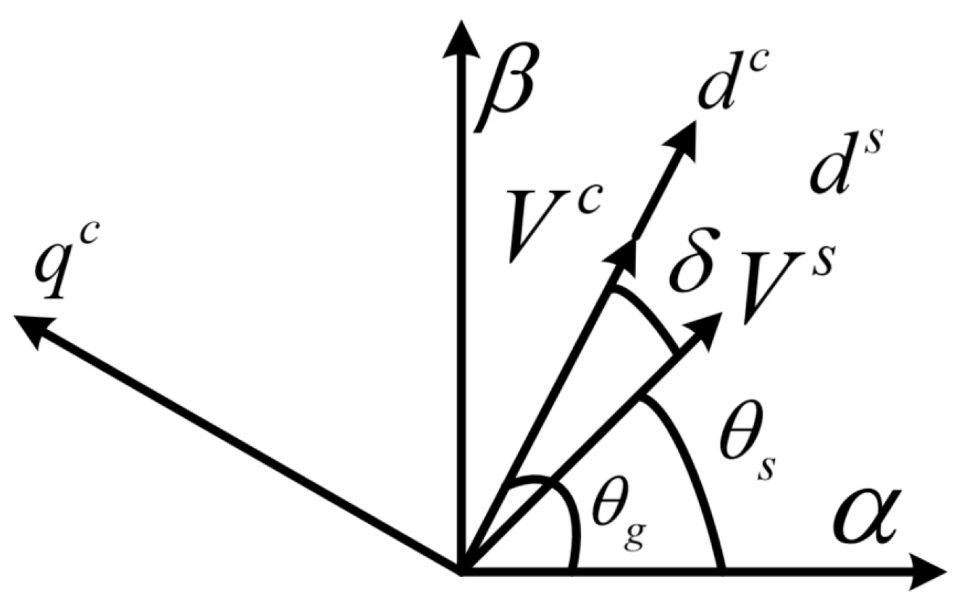
3.1. Principle of VSG Control

The VSG control strategy aims to replicate the inertia and droop characteristics observed in the active power loop of SGs, as well as the voltage-amplitude droop characteristic present in the reactive power loop of SGs. To achieve this, an output voltage reference value was provided, and the inner loop was employed for voltage construction and tracking. The inner loop control methods for VSG control can be classified into three categories: direct duty cycle control, voltage single-loop control, and voltage-current double loop control methods. The first method, direct duty cycle control, is essentially an open-loop control method and is limited in practical applications. The single-loop control method, although effective in voltage control, fails to achieve current limitations during faults. In this paper, the voltage-current double-loop control method was adopted for the inner loop. This method has been proven to be effective and reliable in practical applications, as it addresses the limitations of the other control methods and ensures both voltage and current regulation.

As shown in Figure 1, the VSC output was filtered through an LC filter and then connected to the grid through grid inductance. The VSG control strategy aims to simulate the droop and inertia characteristics of the active power loop in SGs, as well as the voltage droop characteristics in the reactive power loop. Therefore, in the VSG control strategy, the outer active power loop generates the phase-angle reference value, the reactive power loop generates the voltage-magnitude reference value, and then the voltage and current double inner loops are adopted for voltage tracking and construction [28].

For a VSC with grid-forming control to assist in generating AC voltage, it requires a front-end converter or a stable energy system, or a large capacitor on the DC side to provide voltage and power support. As a result, the DC voltage, denoted as $V_{dc}$, can be assumed to remain constant. The Insulated Gate Bipolar Transistor (IGBT) is extensively utilized in diverse power electronic devices and serves as a common switch transistor in grid-connected equipment due to its excellent performance in various applications. Thus, the switch tubes of the VSC in this paper were based with the commonly used IGBT as an example, which are represented by $S_1$–$S_6$. The output side of the VSC was connected to an LC filter, where the inductance is denoted as $L_1$ and the capacitance as $C$. Additionally, there was an impedance in the grid, represented by $L_g$, which was located between the VSC output terminal and the grid. The grid voltage is represented as $v_s$, with an amplitude of $V_s$ and an angle of ${\theta }_s$. The voltage on the capacitor is denoted as $v_c$, with an amplitude of $V_c$ and an angle of ${\theta }_c$. The current on the VSC side is denoted as $i_1$, while the current on the grid side is represented as $i_2$. The voltage across the capacitor is denoted as $v_C$. $P_{ref}$ and $Q_{ref}$ are the reference values for active and reactive power for the outer power loop. $J_p$ and $D_p$ represent the inertia and damping coefficients of the VSG control strategy. Furthermore, $k_q$ is used for voltage-amplitude development. The rated angular frequency is ${\omega }_0=2\pi ·50 \mathrm{rad}/\mathrm{s}$. The angle ${\theta }_g$, obtained from the active power loop, was used for Park transformation and inverse Park transformation. $v_{dref}$ and $v_{qref}$ represent the voltage amplitudes in the d-axis and q-axis, respectively. $v_{dref}$ is determined by the reactive voltage amplitude loop, while $v_{qref}$ was set to zero. Since the control was implemented on the dq-axis, subscripts d and q were used to differentiate the variables. $d_d$ and $d_q$ represent the duty cycle in the d and q axis, respectively. $V_0$ is the voltage-amplitude reference value used in the reactive power control loop. $k_{vp}$ and $k_{vi}$ are the proportional parameter and the integrator parameter of the voltage control loop, and $k_{ip}$ is the proportional parameter of the current control loop. $i_{1dref}$ and $i_{1qref}$ represent the reference value of the inner current loop.

3.2. Model of the VSG Control Strategy

The grid voltage rotates at a constant angular frequency, and the power outer loop dynamically adjusts the reference angular frequency $\omega$ based on the detected power value. In the steady state, $\omega$ equals ${\omega }_0$, but there may be differences between the two angular frequencies during transient processes. The axis system used for positioning the grid voltage is referred to as the s-system, while the axis system generated by the power outer loop’s phase angle is referred to as the c-system. The relative positions of these two systems remain constant in the steady state, but may deviate from each other during transient processes. The relative schematic diagram is illustrated in Figure 2. The power angle $\delta$ is defined as the angle between the s-system and the c-system, where $\delta ={\theta }_g-{\theta }_s$.

The transformation of the state variable expressions from the c-system to the s-system can be derived as follows, where the state variables projected onto the c-system and s-system are represented, respectively, with superscripts c and s:

$$x_{d,q}^c=e^{j-\delta }{x}_{d,q}^s=\left(cos\delta -jsin\delta \right)·\left(x_d^s+j{x}_q^s\right).$$

(17)

Thus, it can be deduced that:

$$\left\{\begin{array}{c}{x}_d^c=cos\delta x_d^s+sin\delta x_q^s\\ x_q^c=cos\delta x_q^s-sin\delta x_d^s\end{array}\right.,$$

(18)

$$\left\{\begin{array}{c}{x}_d^c=cos\delta x_d^s+sin\delta x_q^s\\ x_q^c=cos\delta x_q^s-sin\delta x_d^s\end{array}\right..$$

(19)

The state-space model for the circuit part can be derived as follows:

$$\left\{\begin{array}{c}{L}_1\frac{d{i}_{1d}^s}{dt}=d_d^s{V}_{dc}-v_{cd}^s+{\omega }_0{L}_1{i}_{1q}^s\\ L_1\frac{d{i}_{1q}^s}{dt}=d_q^s{V}_{dc}-v_{cq}^s-{\omega }_0{L}_1{i}_{1d}^s\\ C\frac{d{v}_{cd}^s}{dt}=i_{1d}^s-i_{2d}^s+{\omega }_{0}C{v}_{cq}^s\\ C\frac{d{v}_{cq}^s}{dt}=i_{1q}^s-i_{2q}^s-{\omega }_{0}C{v}_{cd}^s\\ L_g\frac{d{i}_{2d}^s}{dt}=v_{cd}^s-v_{sd}^s+{\omega }_0{L}_g{i}_{2q}^s\\ L_g\frac{d{i}_{2q}^s}{dt}=v_{cq}^s-v_{sq}^s-{\omega }_0{L}_g{i}_{2d}^s\end{array}\right..$$

(20)

For power calculation, it can be modeled as

$$p=1.5\left(v_{cd}^c{i}_{2d}^c+v_{cq}^c{i}_{2q}^c\right),$$

(21)

$$q=1.5\left(v_{cq}^c{i}_{2d}^c-v_{cd}^c{i}_{2q}^c\right).$$

(22)

As illustrated in Figure 1, the active power control part can be deduced as follows:

$$\frac{d\omega }{dt}=\frac{1}{J_p}\left[P_{ref}-p-D_p\left(\omega -{\omega }_0\right)\right].$$

(23)

The angle reference can be obtained by integrating the frequency, which can be expressed as:

$${\theta }_g=\int \omega dt=\int \left({\omega }_0+\Delta \omega \right)dt.$$

(24)

The voltage-amplitude reference of VSG can be modeled as:

$$v_{dref}=V_0+\left(1/k_q\right)\left(Q_{ref}-q\right).$$

(25)

The inner control loop, depicted in Figure 1, can be modeled as:

$$\left\{\begin{array}{c}\frac{d{x}_{vd}^c}{dt}=k_{vi}\left(v_{dref}-v_{cd}^c\right)\\ \frac{d{x}_{vq}^c}{dt}=k_{vi}\left(v_{qref}-v_{cq}^c\right)\\ i_{1dref}^c=x_{vd}^c+k_{vp}\left(v_{dref}-v_{cd}^c\right)\\ i_{1qref}^c=x_{vq}^c+k_{vp}\left(v_{qref}-v_{cq}^c\right)\\ d_d^c=k_{ip}\left(i_{1dref}^c-i_{1d}^c\right)\\ d_q^c=k_{ip}\left(i_{1qref}^c-i_{1q}^c\right)\end{array}\right.,$$

(26)

where $x_{vd}^c$ and $x_{vq}^c$ are the state variables introduced by the integrators of the voltage PI controllers. Combing (17)–(26), the full-order model of the VSG was developed.

3.3. Transient Stability Analysis for Grid-Forming VSCs

The state variables can be separated into steady-state values and dynamic values. For example, $\delta ={\theta }_g-{\theta }_s={\delta }^{*}+\mathsf{\Delta }\delta ={\mathsf{\Theta }}_g+\mathsf{\Delta }{\theta }_g-{\mathsf{\Theta }}_s-\mathsf{\Delta }{\theta }_s={\delta }^{*}+\mathsf{\Delta }{\theta }_g-\mathsf{\Delta }{\theta }_s={\delta }^{*}+\mathsf{\Delta }{\theta }_g$, where ${\delta }^{*}$ represents the steady-state value of the power angle and $\mathsf{\Delta }\delta$ represents the dynamic value. Since the grid voltage rotates at a constant angular frequency, $\mathsf{\Delta }{\theta }_s=0$.

In the transient stability analysis of nonlinear systems, the stable operating point is often defined as the origin, which is used to determine if the initial point falls within the ROA. When dealing with trigonometric functions in the nonlinear model, Taylor series expansion can be utilized to approximate them. This enables expressing them as follows:

$$cos\delta =cos\left({\delta }^{*}\right)-sin\left({\delta }^{*}\right)\mathsf{\Delta }\delta -\frac{1}{2}cos\left({\delta }^{*}\right){\left(\mathsf{\Delta }\delta \right)}^2+\dots ,$$

(27)

$$sin\delta =sin\left({\delta }^{*}\right)+cos\left({\delta }^{*}\right)\mathsf{\Delta }\delta -\frac{1}{2}sin\left({\delta }^{*}\right){\left(\mathsf{\Delta }\delta \right)}^2-\frac{1}{3!}cos\left({\delta }^{*}\right){\left(\mathsf{\Delta }\delta \right)}^3+\dots .$$

(28)

By combining Equations (17)–(28), a truncated model of a grid-forming VSC can be obtained, which represents a more concrete version of (2). Therefore, the nonlinear decoupling method can be employed to analyze the transient stability of the system.

3.4. Typical Cases for Transient Stability Analysis

In the study of transient stability, the impact of various typical parameters in grid-forming converters was examined. This analysis aims to provide guidelines for designing parameters that prioritize transient stability.

Table 2. Parameters of VSGs.

Symbol	Parameters	Value
$P_{ref},Q_{ref}$	Reference of active and reactive power	40 kW, 0 kVar
$J_p$	Virtual inertia	200 kg·m2
$D_p$	Damping coefficient	800 (N·m·s)/rad
$k_q$	Reactive-voltage droop coefficient	800 Var/V
$V_{dc}$	The voltage of the DC side	1000 V
$L_1,C,L_g$	Inductance and capacitance	5 mH, 200 uF, 4 mH
$K_{vp},K_{vi},K_{ip}$	Proportional and integral parameters	1, 100, 0.005

presents the parameters considered for the VSG, excluding any parameters specifically noted as varying in the different cases. The parameter-design problem of VSCs is a comprehensive and difficult issue. There have been numerous studies on this topic in the existing literature [31,32]. However, it is not the main focus of this paper and, therefore, will not be discussed in detail.

Case I: System transient stability under varying voltage-amplitude drops

This paper focuses on studying the transient stability of the system when experiencing sudden drops in grid voltage amplitude, which represents a significant disturbance that the system may encounter. By utilizing the developed model and the nonlinear decoupling method, the transient stability of the original system was analyzed by combining the decoupled modes and their corresponding initial points. This analysis was conducted for different degrees of voltage-amplitude drop in the power grid. Due to space constraints, this paper presents only the ROAs and initial points corresponding to the critical modes.

According to Figure 3, as the voltage-amplitude drop intensifies, the ROA for the critical mode significantly decreases, and the initial operating points move toward the outer limits. In the event of a sudden drop in the system voltage amplitude to half of its steady-state value, the initial point falls outside the ROA, suggesting an imminent system instability.

Case II: Influence of parameters in the active power control loop on transient stability

During large disturbances, such as voltage-amplitude drops, the transient behavior of systems with varying inertia and damping coefficients will differ. Figure 4a,b illustrate the critical modes and initial points for different inertia and damping parameters in the extreme scenario where the voltage amplitude decreases to half.

According to Figure 4, the behavior of the system is influenced by the damping and inertia parameters. As the damping and inertia parameters increase, the initial operation points of the system exhibit minimal changes, but the size of the ROAs displays the opposite trend. The ROA of the system expands continuously with increasing damping parameters. Once the damping parameter reaches a value of 1200 (N·m·s)/rad, the initial points fall within the ROA, indicating that increasing damping can enhance the transient stability of the system. On the other hand, when the inertia parameters increase, although the initial point tends to approach the origin, the ROAs shrink at a faster rate. Therefore, a higher inertia coefficient negatively impacts the transient stability of the system.

In practical applications, it is common to employ large inertia parameters to mitigate frequency fluctuations in a system during disturbances. This approach aims to enhance system frequency stability and prevent the system operation frequencies from exceeding the predetermined threshold. However, it is important to strike a balance between frequency stability and transient stability when designing the inertia parameters.

Case III: Influence of parameters in reactive power control loops on transient stability

The study of transient stability has predominantly focused on the influence of the outer active power loop. Nevertheless, it is worth noting that the parameters associated with the reactive power control loop can also have an impact on the transient stability of the system. This paper addresses this aspect by examining the ROAs and initial points for various voltage-droop coefficients and reactive power reference values.

Based on the analysis of Figure 5a, it can be observed that as the voltage-droop coefficients increase, the ROAs expand significantly, and the position of the initial point moves inward. These findings indicate that increasing this parameter is beneficial for enhancing the transient stability of the system. Furthermore, Figure 5b demonstrates that as the reference values of the reactive power gradually increase, the position of the initial points almost remains unchanged, while the ROAs gradually expand. This observation suggests that appropriately increasing the VSC’s reactive power transfer can effectively maintain the transient stability of the system, particularly during large disturbances.

Case IV: Influence of inner loop parameters on transient stability

The existing literature predominantly utilizes quasi-steady-state models for grid-forming VSGs to analyze transient stability, disregarding the impact of the complete inner loop. Consequently, the transient stability of the system can only be examined with different outer loop parameters. This paper addresses this limitation by developing a comprehensive and full-order model of grid-forming VSCs. The nonlinear decoupling method was employed to separate the high-order model into multiple low-order modes, enabling an analysis of the influence of internal loop parameters on transient stability.

Based on the analysis of the ROAs and corresponding initial points displayed in Figure 6, it is evident that when the parameters of the inner loop are altered, the ROAs and initial points of the system can undergo substantial variations, ultimately leading to different levels of transient stability. In contrast, the adoption of the quasi-steady-state model and stability analysis method described in [28] allows the system to sustain transient stability under a particular set of outer loop parameters. However, this approach fails to provide insights into the specific impacts of inner loop parameters on stability.

4. Discussions

The conventional analysis process for high-order nonlinear systems is limited by the available transient stability analysis tools. Therefore, a corresponding quasi-steady-state model is commonly developed for grid-forming VSCs, and the phase diagram of the system operation trajectory is utilized to evaluate the transient dynamics of low-order systems [28]. For comparison, the commonly used quasi-steady-state model was established and derived to illustrate its limitations in the modeling process.

Considering (23) and (24), the active power control loop can be modeled as:

$$\frac{d^2\delta }{d{t}^2}=\frac{1}{J_p}\left[P_{ref}-p-D_p\frac{d\delta }{dt}\right]$$

(29)

The model of the reactive power outer loop is the same as (25). The grid voltage is denoted as $v_s$, and the voltage on the capacitor side is represented as $v_C$. The grid impedance, $X_g=\omega L_g$, is located between the capacitor and the grid. The active and the reactive power transferred between the VSC and the grid can be calculated as:

$$p=\frac{3V_s{V}_C}{2X_g}sin\left(\delta \right)$$

(30)

$$q=\frac{3V_C\left(V_C-V_{s}cos\left(\delta \right)\right)}{2X_g}$$

(31)

In conventional transient stability analysis for grid-forming VSCs, to simplify the analysis, it was assumed that the inner control loop was fast enough to neglect the influence of its dynamics. Thus, it was assumed that $V_C=V_{dref}$. Therefore, substituting (31) into (25), it can be obtained as:

$$V_{dref}=\left(\frac{1}{2}{V}_{s}cos\left(\delta \right)-\frac{1}{3}{k}_q{X}_g\right)+\sqrt{{\left(\frac{1}{2}{V}_{s}cos\left(\delta \right)-\frac{1}{3}{k}_q{X}_g\right)}^2+\frac{2}{3}{X}_g{Q}_{ref}+\frac{2}{3}{X}_g{k}_q{V}_0}$$

(32)

Combining (32), (29), and (30), the two-order model for the power angle can be derived as:

$$\begin{gathered} \frac{d^2\delta }{d{t}^2}=\frac{1}{J_p}\left\{P_{ref}-\frac{3V_s}{2X_g}sin\left(\delta \right)\left[\left(\frac{1}{2}{V}_{s}cos\left(\delta \right)-\frac{1}{3}{k}_q{X}_g\right)+ \\ \sqrt{{\left(\frac{1}{2}{V}_{s}cos\left(\delta \right)-\frac{1}{3}{k}_q{X}_g\right)}^2+\frac{2}{3}{X}_g{Q}_{ref}+\frac{2}{3}{X}_g{k}_q{V}_0}\right]-D_p\frac{d\delta }{dt}\right\} \end{gathered}$$

(33)

Therefore, the current analysis method mainly focuses on deriving a second-order quasi-steady-state model for grid-forming VSCs, as shown in (33), and using phase plane analysis to determine the transient stability of the system under different parameters. Clearly, this model neglects the influence of inner loop control and the converter circuit on transient stability, which may result in deviations in the analysis results.

Under the same set of parameters, the system trajectory obtained based on the quasi-steady-state model is shown in Figure 7.

According to Figure 7, by utilizing the quasi-steady-state model under the same set of parameters, the phase diagram track of the power angle was plotted. It is evident that the system eventually converges to a new stable operating point after undergoing multiple oscillations. However, due to the neglect of the inner control loop in this modeling approach, variations in inner loop parameters do not affect the analysis results. Therefore, in comparison, the full-order model and the nonlinear decoupling method can accurately analyze the transient instability phenomenon that the system may experience.

This section analyzes the impact of different parameters on transient stability through multiple case studies, as summarized in

Table 3. Impact of parameters on transient stability.

Parameters	Impact on Transient Stability
Voltage-amplitude sag	The greater the voltage magnitude drop, the more likely the system is to experience transient instability.
Active power control loop parameters	Increasing the damping coefficient contributes to transient stability in the system, while increasing the inertia coefficient may lead to transient instability in the system.
Reactive power control loop parameters	Increasing the voltage-reactive power droop coefficient and reactive power reference value helps to improve the transient stability of the system.
Inner loop control parameters	The control parameters of the current inner loop result in significant changes to the stability region of the system, and excessively small control parameters of the current inner loop may lead to transient instability in the system.

.

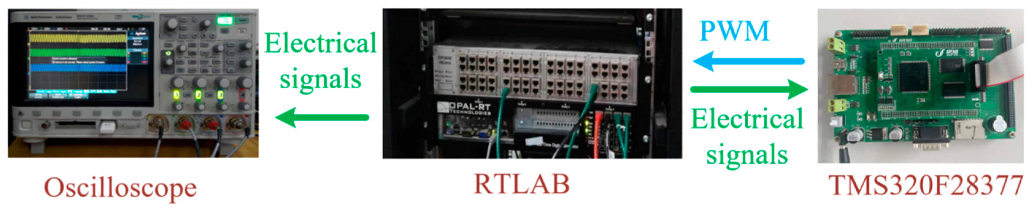
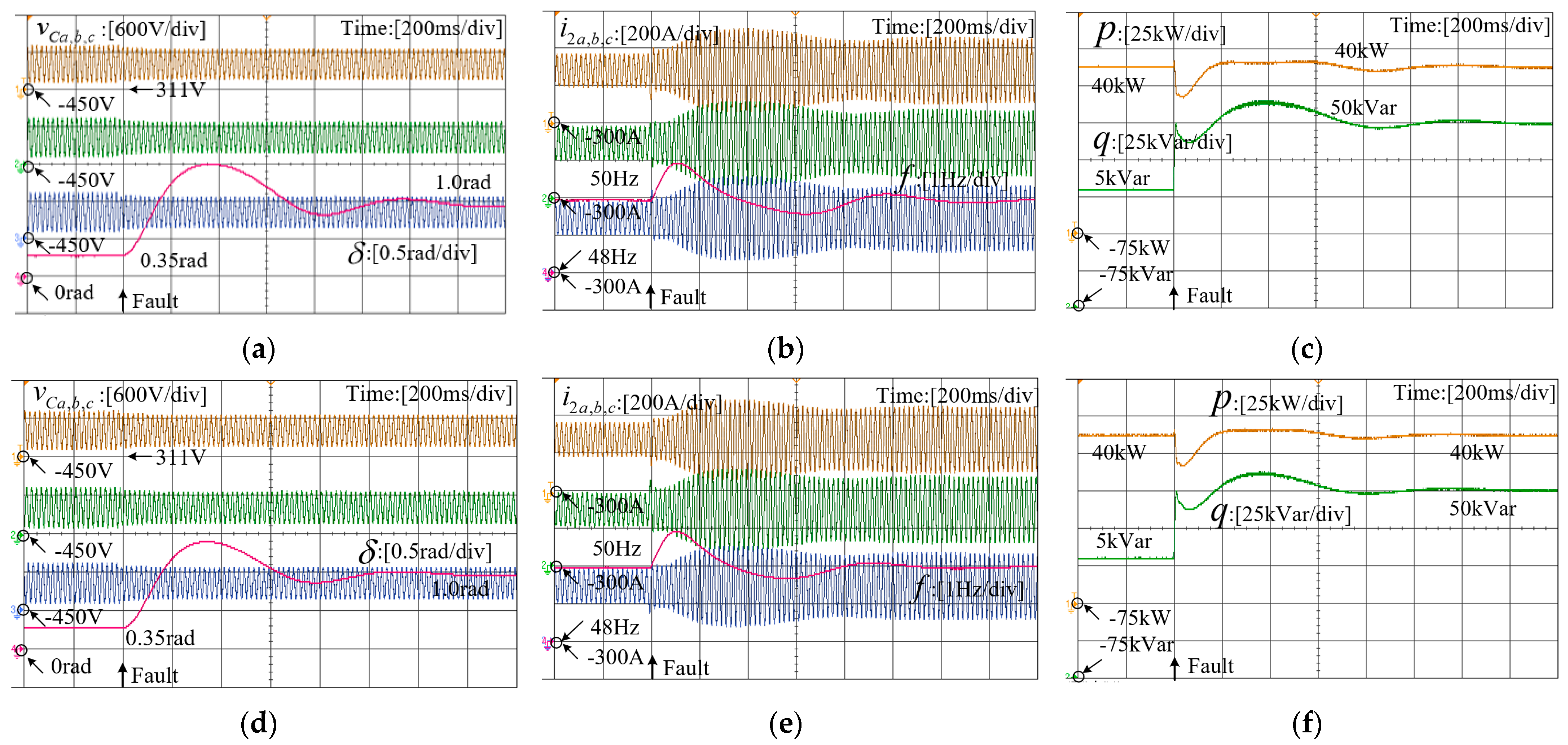
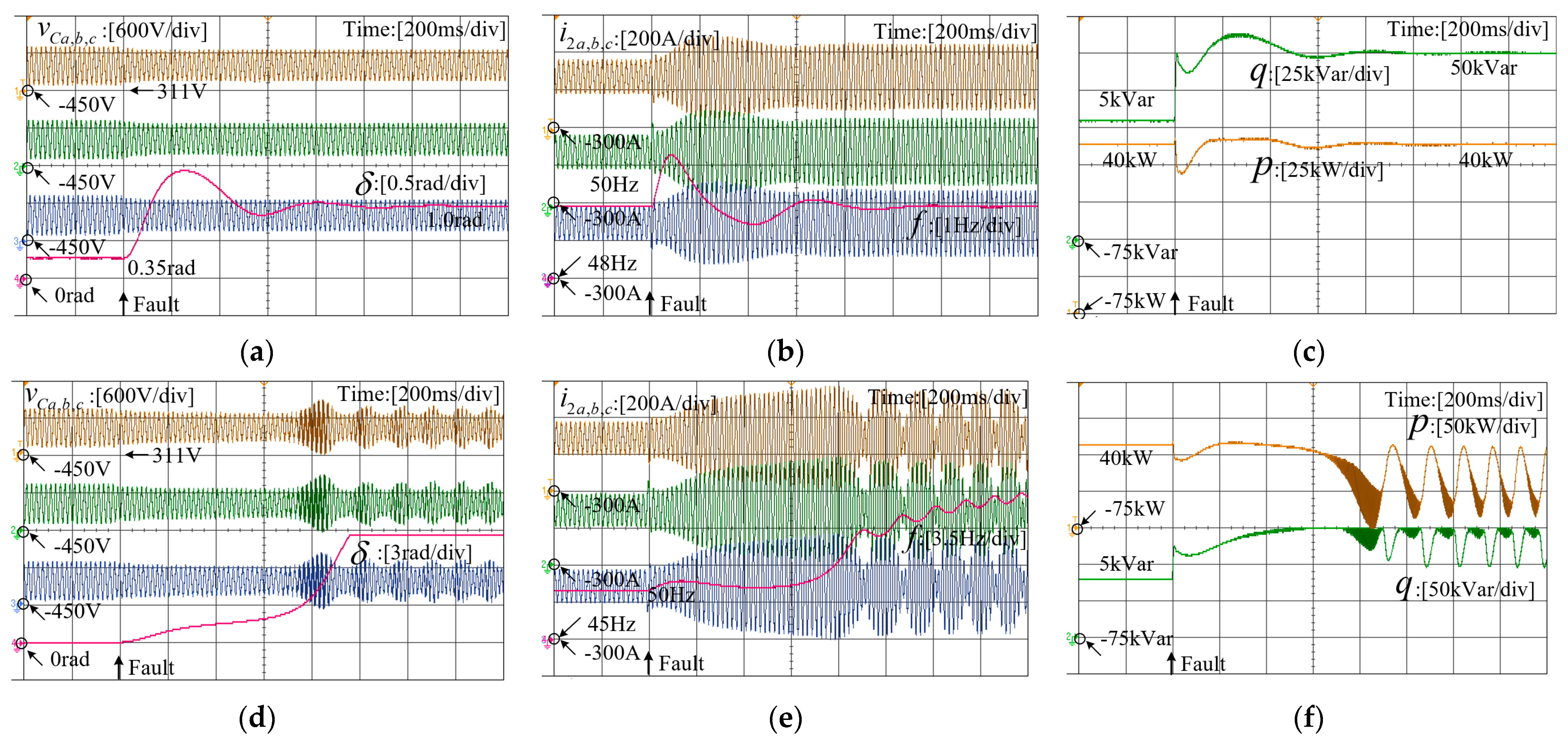
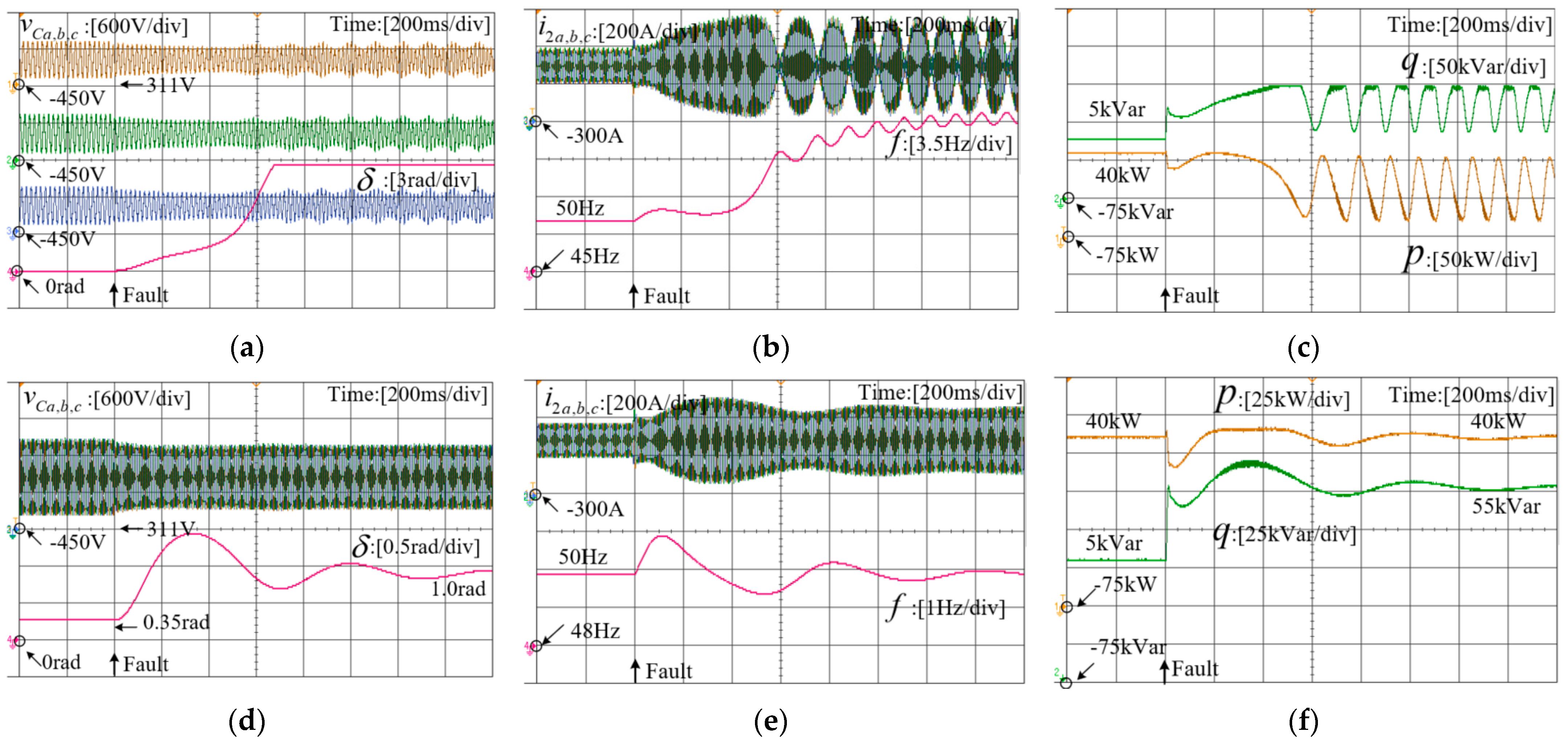
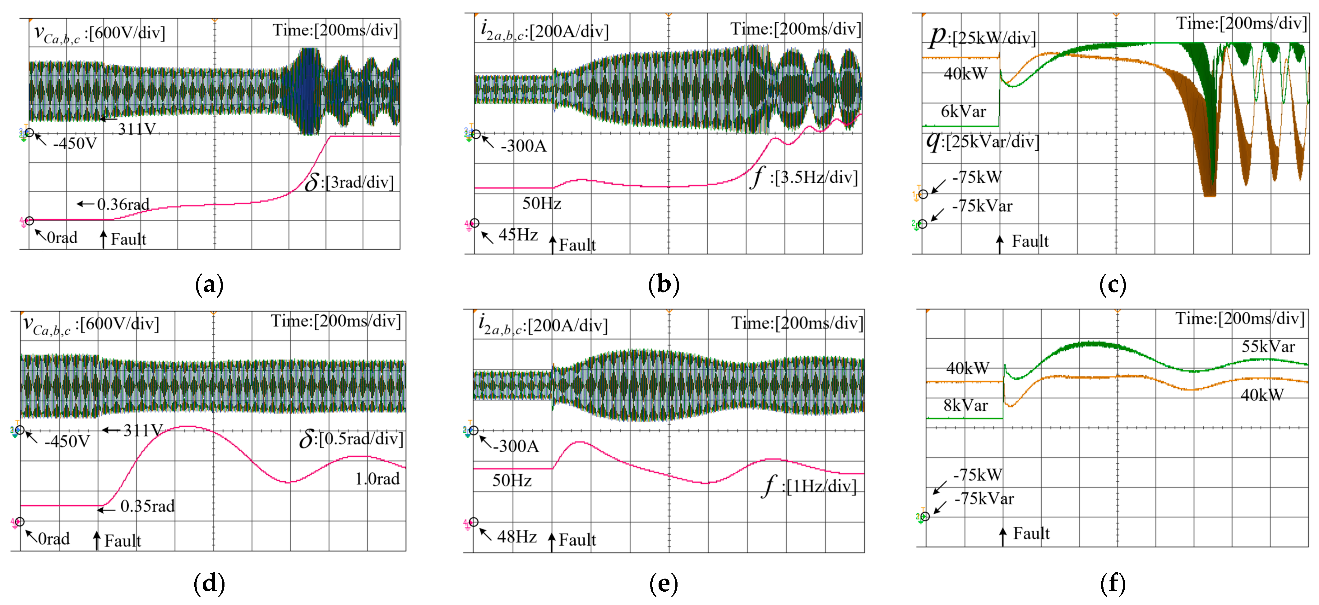
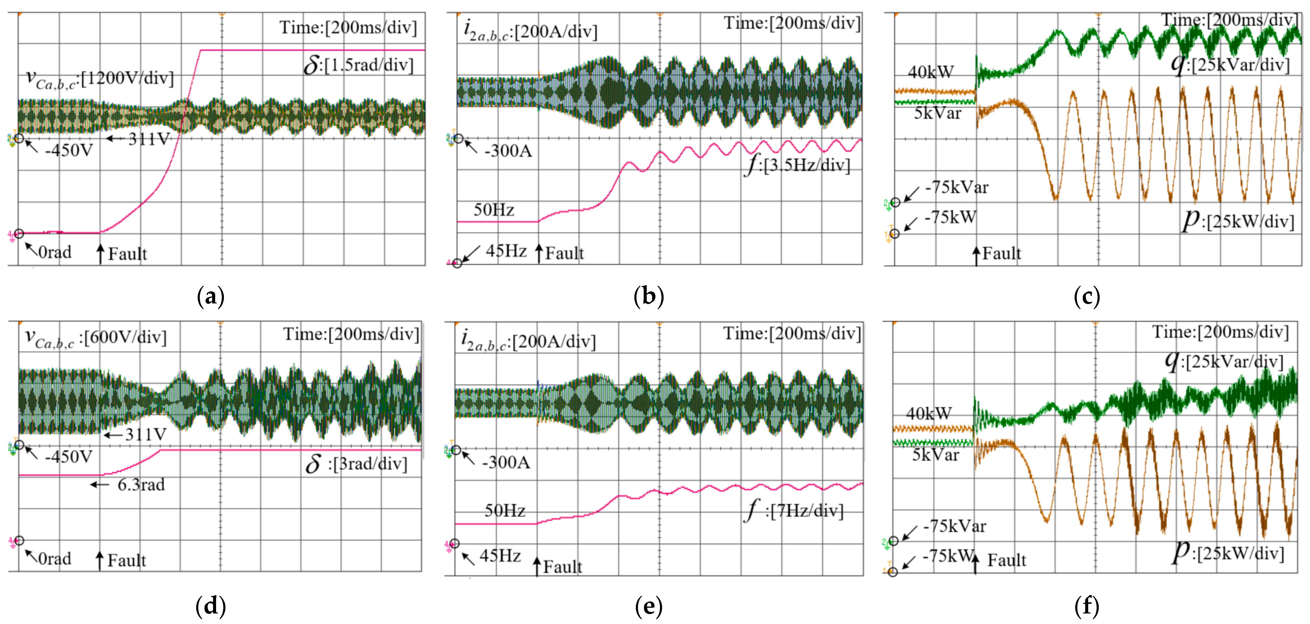
5. HIL Experiment Verification

To validate the conclusions of the transient stability analysis of grid-forming VSCs, HIL experiments were conducted to verify the analysis cases. The experimental facilities are shown in Figure 8, including the real-time simulator RTLAB, the TMS320F28377 DSP, and the oscilloscope. The primary section of the VSC was simulated in real-time using RTLAB, while the control algorithm was implemented in the DSP controller. The development board integrated A/D and D/A conversion modules for electrical signal sampling and sent PWM signals back to RTLAB to control the switching devices of the VSC. An oscilloscope was used to record the signals that needed to be observed.

Case I: Transient stability experiments with different voltage-amplitude sags

HIL experiments were conducted to assess the transient stability of the system under varying grid voltage-amplitude sags, including voltage sags of 0.8 pu, 0.6 pu, and 0.5 pu. The rated voltage amplitude was 311 V, and the parameters used in the VSC mirrored those in Table 2. Figure 9 displays the voltage waveforms of the capacitor, system power angle, active and reactive power output, as well as the three-phase current waveforms during significant disturbances.

According to Figure 9, when the voltage amplitude of the power grid experiences a minor decrease, the system can easily return to the steady-state operation point following a brief period of oscillation. This indicates that the system is capable of maintaining transient stability. However, as the voltage amplitude drops further, the fluctuations in power angle, frequency, and output power become more pronounced. When the voltage amplitude reaches 0.5 pu, both the power angle and frequency continue to increase, leading to sustained oscillations within the system. This observation suggests that the VSG is no longer synchronized with the power grid, resulting in transient instability within the system.

Case II: Influence of parameters in the active power control loop on transient stability

In line with the analysis conducted in Section 3, it was observed that the damping and inertia parameters within the active power control loop significantly influenced the transient stability of the VSG. This influence is depicted in the experimental waveforms presented in Figure 10.

Based on the information provided by Figure 10, it is evident that enhancing the damping parameter of the system improves the transient stability compared with the system with a smaller damping parameter shown in Figure 9g–i. Furthermore, as the damping parameter increases, the maximum overshoot of the system power angle and frequency progressively decreases.

By combining Figure 9g–i and Figure 11, it was observed that increasing the inertia parameter of the system led to transient instability, as indicated by the divergence of power angle rates. While a higher inertia parameter can help mitigate frequency fluctuations during disturbances, it is not conducive to maintaining the transient stability of the system.

Case III: Influence of parameters in reactive power control loop on transient stability

The transient performance of the system was influenced by the parameters of the reactive power loop, as the active and reactive power loops were coupled in the control of the VSG. Figure 12 and Figure 13 display waveforms captured under various reactive power loop configurations.

By combining Figure 9g–i and Figure 12, it was observed that when the voltage droop coefficient was small, the voltage reference values decreased significantly under the same disturbance. Consequently, the power angle was unable to recover to the steady-state operation point. As a result, the system experienced continuous oscillation and lost transient stability.

Combining Figure 11d–f and Figure 13, it is evident that, with the other parameters held constant, increasing the reactive power reference value facilitates the system returning to the steady-state operation point. Consequently, appropriately manipulating reactive power transfer can enhance the system’s resilience against significant disturbances.

Case IV: Influence of inner loop parameters on transient stability

Conventional analysis methods often simplify the inner control loop of high-order systems by considering it as a unit gain, thereby disregarding the influence of the inner loop on transient stability. However, experiments demonstrate that the transient stability of the system is indeed affected by various inner loop parameters, as depicted in Figure 14.

Based on Figure 14, it was observed that relying solely on the oversimplified model focusing on the outer power control loop may lead to the incorrect conclusion that the system can maintain transient stability during voltage-amplitude drops. However, when the inner control parameters are modified while keeping the outer loop parameters constant, transient instability arises. This transient instability phenomenon exhibited in the experiments aligns with the analysis results presented in Figure 6.

6. Conclusions

This paper presents the development of a full-order large signal model for grid-forming VSCs and applies a nonlinear decoupling method to decompose the high-order system into multiple low-order modes. The transient stability of the original system was indirectly assessed by employing the inverse trajectory method for the low-order modes. HIL experiments were conducted to validate the theoretical analysis findings. The main conclusions of the transient stability analysis for grid-forming inverters are as follows:

(1)

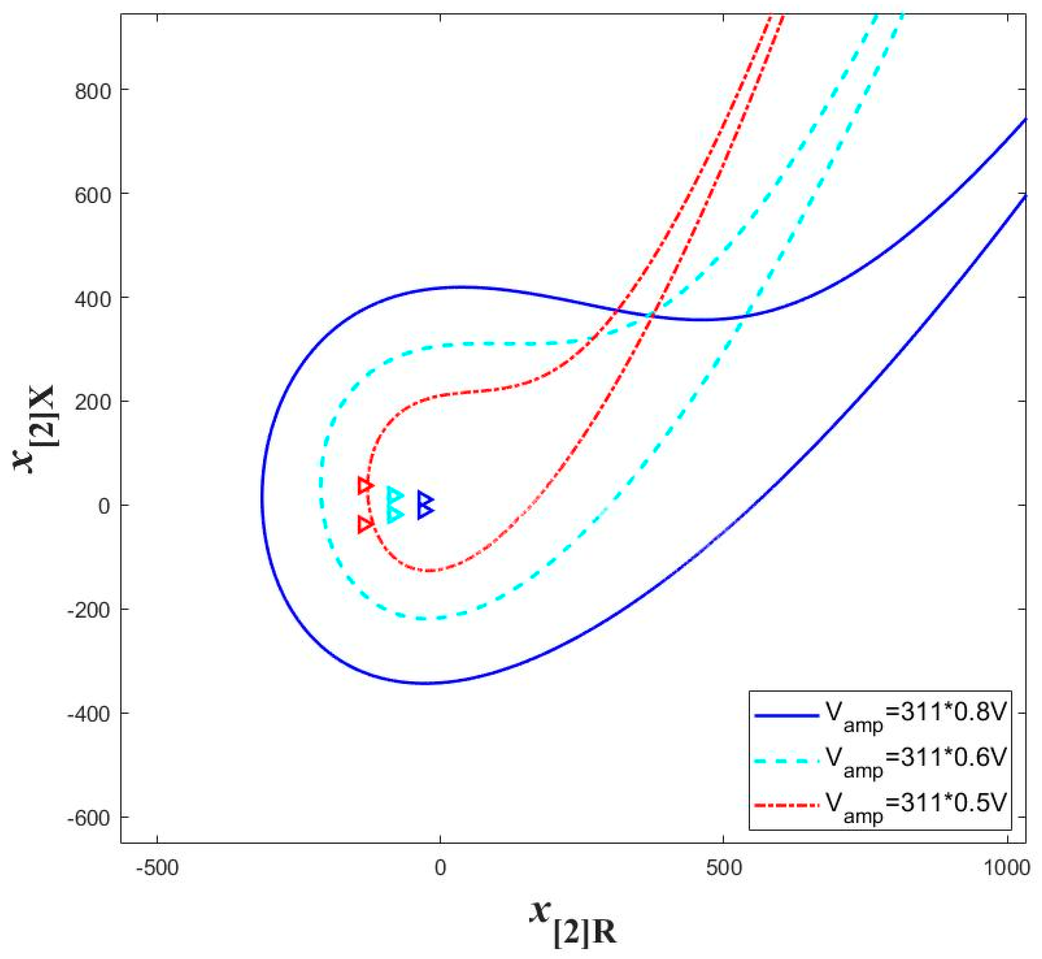
The transient stability of grid-forming inverters diminishes with increasing voltage-amplitude drop in the grid. In essence, a larger magnitude of voltage drop in the grid corresponds to a higher likelihood of transient instability occurring in the system.

(2)

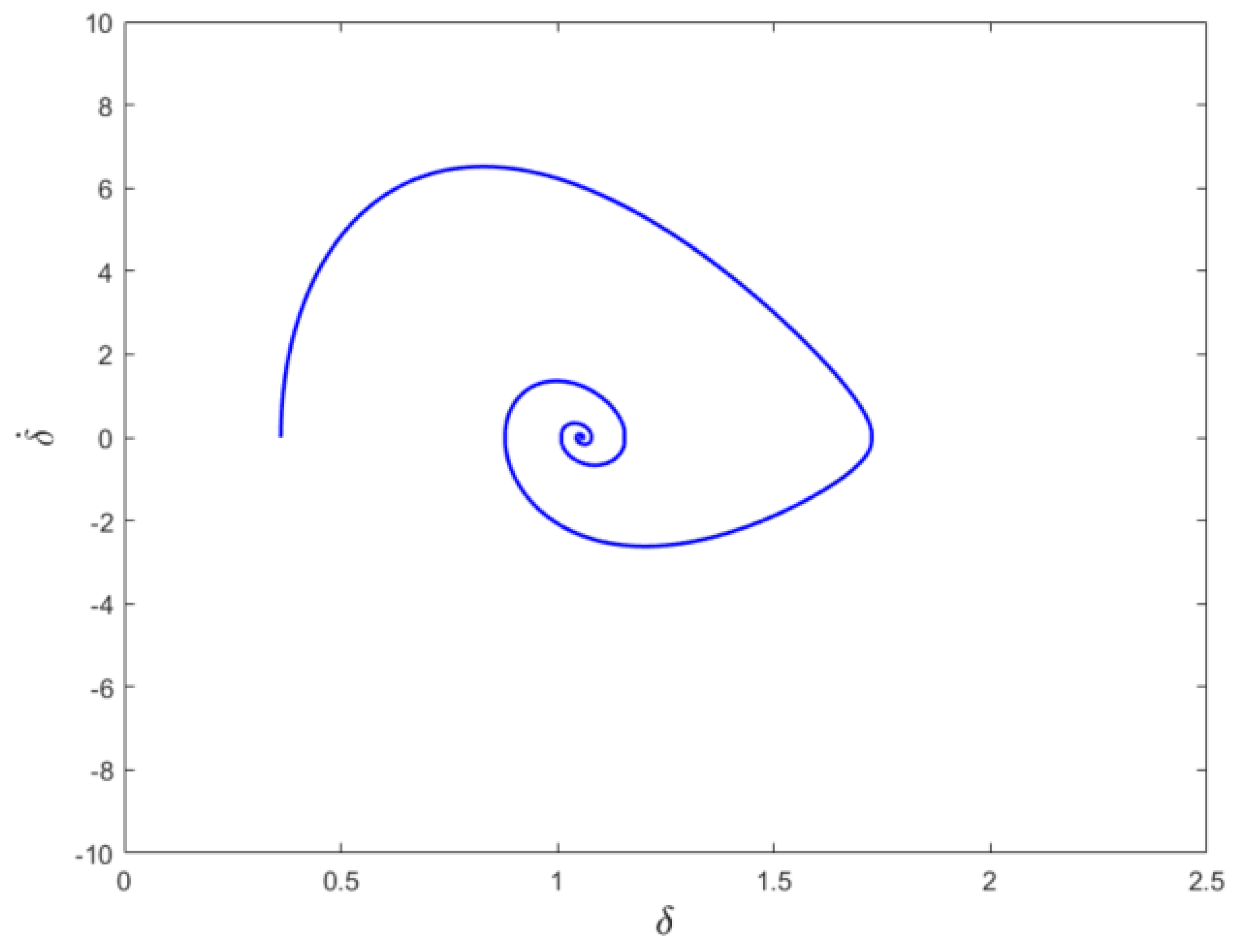
The analysis demonstrates that the damping parameters and inertia parameters within the active power loop exert varying influences on the transient stability of grid-forming VSCs. A larger damping parameter effectively mitigates power-angle fluctuations, facilitating the restoration of steady-state operation points. Conversely, a higher inertia parameter narrows the ROA of the critical mode, thereby diminishing the system’s transient stability.

(3)

Furthermore, the impact of parameters in the reactive power loop on transient stability was also examined. An increased voltage-drop coefficient and reactive power reference value are shown to enhance transient stability.

(4)

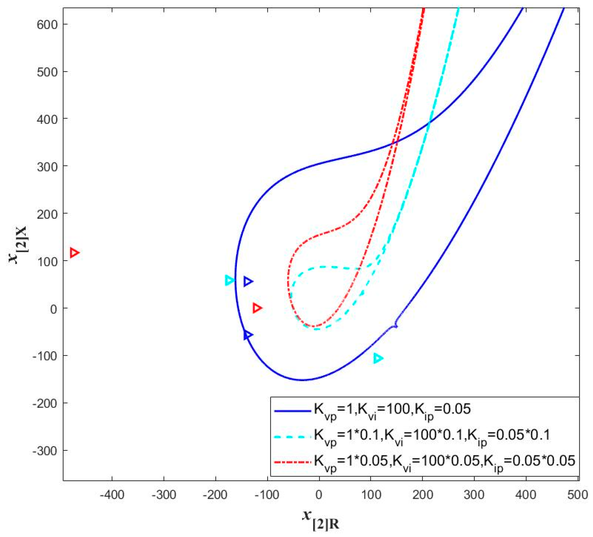
In the existing literature, the transient stability analysis of grid-forming VSCs relies on establishing a quasi-steady-state model that exclusively focuses on the outer control loop. This approach is relatively accurate when there is a significant difference in bandwidth between the inner and outer loops. However, current methods completely disregard the impact of the inner control loop, rendering them unable to analyze the transient stability of the system when the inner loop parameters change. In this paper, the method for developing the quasi-steady-state model based on the existing literature is presented. Subsequently, the existing method is used to analyze the transient stability with the same parameters, and the obtained results are compared with the stability analysis results of the full-order model adopted in this paper. The comparison indicates that the proposed method offers a more comprehensive approach to transient analysis for grid-forming VSC systems.

References

1. D’Adamo, I.; Mammetti, M.; Ottaviani, D.; Ozturk, I. Photovoltaic systems and sustainable communities: New social models for ecological transition. The impact of incentive policies in profitability analyses. Renew. Energy 2023, 202, 1291–1304. [Google Scholar] [CrossRef]
2. Olabi, A.G.; Obaideen, K.; Abdelkareem, M.A.; AlMallahi, M.N.; Shehata, N.; Alami, A.H.; Mdallal, A.; Hassan, A.A.M.; Sayed, E.T. Wind Energy Contribution to the Sustainable Development Goals: Case Study on London Array. Sustainability 2023, 15, 4641. [Google Scholar] [CrossRef]
3. Kumar, R.; Kumar, A.; Gupta, M.K.; Yadav, J.; Jain, A. solar tree-based water pumping for assured irrigation in sustainable Indian agriculture environment. Sustain. Prod. Consum. 2022, 33, 15–27. [Google Scholar] [CrossRef]
4. Kumar, R.; Pachauri, R.K.; Badoni, P.; Bharadwaj, D.; Mittal, U.; Bisht, A. Investigation on parallel hybrid electric bicycle along with issuer management system for mountainous region. J. Clean. Prod. 2022, 362, 132430. [Google Scholar] [CrossRef]
5. Raupp, I.P.; da Paz, L.R.L.; da Serra Costa, F.; de Matos, D.F.; Garcia, K.C. Key challenges of sustainable hydropower in the context of energy transition: A Brazilian contribution. In Renewable Energy Production and Distribution; Jeguirim, M., Dutournié, P., Eds.; Academic Press: Cambridge, MA, USA, 2023; Volume 2, pp. 315–349. [Google Scholar]
6. Costa, J.; Kilajian, A.; Kadyrzhanova, A. Hydropower Sustainability Assessment. Comprehensive Renewable Energy, 2nd ed.; Letcher, T.M., Ed.; Elsevier: Amsterdam, The Netherlands, 2022; pp. 202–224. [Google Scholar]
7. Kondrakhin, V.P.; Martyushev, N.V.; Klyuev, R.V.; Sorokova, S.N.; Efremenkov, E.A.; Valuev, D.V.; Mengxu, Q. Mathematical Modeling and Multi-Criteria Optimization of Design Parameters for the Gyratory Crusher. Mathematics 2023, 11, 2345. [Google Scholar] [CrossRef]
8. Meera, C.S.; Sunny, S.; Singh, R.; Sairam, P.S.; Kumar, R.; Emannuel, J. Automated precise liquid transferring system. In Proceedings of the 2014 IEEE 6th India International Conference on Power Electronics (IICPE), Kurukshetra, India, 8–10 December 2014; pp. 1–6. [Google Scholar]
9. Xia, Y.; Wei, W.; Yu, M.; Wang, X.; Peng, Y. Power Management for a Hybrid AC/DC Microgrid With Multiple Subgrids. IEEE Trans. Power Electron. 2018, 33, 3520–3533. [Google Scholar] [CrossRef]
10. Xia, Y.; Wei, W.; Yu, M.; Peng, Y.; Tang, J. Decentralized Multi-Time Scale Power Control for a Hybrid AC/DC Microgrid With Multiple Subgrids. IEEE Trans. Power Electron. 2018, 33, 4061–4072. [Google Scholar] [CrossRef]
11. Popella, H.; Hennig, T.; Kaiser, M.; Massmann, J.; Müller, L.; Pfeiffer, R. Necessary development of inverter-based generation with grid forming capabilities in Germany. In Proceedings of the 20th International Workshop on Large-Scale Integration of Wind Power into Power Systems as well as on Transmission Networks for Offshore Wind Power Plants (WIW 2021), Hybrid Conference, Berlin, Germany, 29–30 September 2021; pp. 125–129. [Google Scholar]
12. Noguchi, T.; Tomiki, H.; Kondo, S.; Takahashi, I. Direct power control of PWM converter without power-source voltage sensors. IEEE Trans. Ind. Appl. 1998, 34, 473–479. [Google Scholar] [CrossRef]
13. De Brabandere, K.; Bolsens, B.; Van den Keybus, J.; Woyte, A.; Driesen, J.; Belmans, R. A Voltage and Frequency Droop Control Method for Parallel Inverters. IEEE Trans. Power Electron. 2007, 22, 1107–1115. [Google Scholar] [CrossRef]
14. Liu, J.; Miura, Y.; Ise, T. Comparison of dynamic characteristics between virtual synchronous generator and droop control in inverter-based distributed generators. IEEE Trans. Power Electron. 2016, 31, 3600–3611. [Google Scholar] [CrossRef]
15. Zhong, Q.-C.; Weiss, G. Synchronverters: Inverters that mimic synchronous generators. IEEE Trans. Ind. Electron. 2011, 58, 1259–1267. [Google Scholar] [CrossRef]
16. Xia, Y.; Wei, W.; Long, T.; Blaabjerg, F.; Wang, P. New Analysis Framework for Transient Stability Evaluation of DC Microgrids. IEEE Trans. Smart Grid 2020, 11, 2794–2804. [Google Scholar] [CrossRef]
17. Wang, X.; Taul, M.G.; Wu, H.; Liao, Y.; Blaabjerg, F.; Harnefors, L. Grid-Synchronization Stability of Converter-Based Resources—An Overview. IEEE Open J. Ind. Appl. 2020, 1, 115–134. [Google Scholar] [CrossRef]
18. Yang, P.; Xia, Y.; Yu, M.; Wei, W.; Peng, Y. A Decentralized Coordination Control Method for Parallel Bidirectional Power Converters in a Hybrid AC–DC Microgrid. IEEE Trans. Ind. Electron. 2018, 65, 6217–6228. [Google Scholar] [CrossRef]
19. Wen, B.; Dong, D.; Boroyevich, D.; Burgos, R.; Mattavelli, P.; Shen, Z. Impedance-Based Analysis of Grid-Synchronization Stability for Three-Phase Paralleled Converters. IEEE Trans. Power Electron. 2016, 31, 26–38. [Google Scholar] [CrossRef]
20. Amin, M.; Molinas, M. Small-Signal Stability Assessment of Power Electronics Based Power Systems: A Discussion of Impedance- and Eigenvalue-Based Methods. IEEE Trans. Ind. Appl. 2017, 53, 5014–5030. [Google Scholar] [CrossRef]
21. Wu, H.; Wang, X. Design-Oriented Transient Stability Analysis of PLL-Synchronized Voltage-Source Converters. IEEE Trans. Power Electron. 2020, 35, 3573–3589. [Google Scholar] [CrossRef] [Green Version]
22. He, X.; Tsinghua University; Geng, H.; Ma, S. Transient Stability Analysis of Grid-Tied Converters Considering PLL’s Nonlinearity. CPSS Trans. Power Electron. Appl. 2019, 4, 40–49. [Google Scholar] [CrossRef]
23. Tang, Y.; Tian, Z.; Zha, X.; Li, X.; Huang, M.; Sun, J. An Improved Equal Area Criterion for Transient Stability Analysis of Converter-Based Microgrid Considering Nonlinear Damping Effect. IEEE Trans. Power Electron. 2022, 37, 11272–11284. [Google Scholar] [CrossRef]
24. Pan, D.; Wang, X.; Liu, F.; Shi, R. Transient Stability of Voltage-Source Converters With Grid-Forming Control: A Design-Oriented Study. IEEE J. Emerg. Sel. Top. Power Electron. 2020, 8, 1019–1033. [Google Scholar] [CrossRef]
25. Shuai, Z.; Shen, C.; Liu, X.; Li, Z.; Shen, Z.J. Transient Angle Stability of Virtual Synchronous Generators Using Lyapunov’s Direct Method. IEEE Trans. Smart Grid 2019, 10, 4648–4661. [Google Scholar] [CrossRef]
26. Xiong, X.; Wu, C.; Blaabjerg, F. Effects of Virtual Resistance on Transient Stability of Virtual Synchronous Generators Under Grid Voltage Sag. IEEE Trans. Ind. Electron. 2022, 69, 4754–4764. [Google Scholar] [CrossRef]
27. Chen, S.; Sun, Y.; Han, H.; Fu, S.; Luo, S.; Shi, G. A Modified VSG Control Scheme With Virtual Resistance to Enhance Both Small-Signal Stability and Transient Synchronization Stability. IEEE Trans. Power Electron. 2023, 38, 6005–6014. [Google Scholar] [CrossRef]
28. Ge, P.; Tu, C.; Xiao, F.; Guo, Q.; Gao, J. Design-Oriented Analysis and Transient Stability Enhancement Control for a Virtual Synchronous Generator. IEEE Trans. Ind. Electron. 2023, 70, 2675–2684. [Google Scholar] [CrossRef]
29. Koditschek, D.; Narendra, K. The stability of second-order quadratic differential equations. IEEE Trans. Autom. Control 1982, 27, 783–798. [Google Scholar] [CrossRef] [Green Version]
30. Tian, T.; Kestelyn, X.; Thomas, O.; Amano, H.; Messina, A.R. An Accurate Third-Order Normal Form Approximation for Power System Nonlinear Analysis. IEEE Trans. Power Syst. 2018, 33, 2128–2139. [Google Scholar] [CrossRef] [Green Version]
31. Wu, H.; Ruan, X.; Yang, D.; Chen, X.; Zhao, W.; Lv, Z.; Zhong, Q.-C. Small-Signal Modeling and Parameters Design for Virtual Synchronous Generators. IEEE Trans. Ind. Electron. 2016, 63, 4292–4303. [Google Scholar] [CrossRef]
32. Pan, D.; Ruan, X.; Bao, C.; Li, W.; Wang, X. Optimized Controller Design for LCL-Type Grid-Connected Inverter to Achieve High Robustness Against Grid-Impedance Variation. IEEE Trans. Ind. Electron. 2015, 62, 1537–1547. [Google Scholar] [CrossRef]
Figure 1. Topology and control strategy of the VSG.
Sustainability 15 11981 g001
Figure 2. Schematic diagram between the s-system and the c-system.
Sustainability 15 11981 g002
Figure 3. ROAs and corresponding initial points of the critical mode for different voltage drops.
Sustainability 15 11981 g003
Figure 4. ROAs and corresponding initial points of the critical mode with different parameters in the active power control loop. (a) Transient stability with different damping coefficients, where the inertia parameter is J p = 200   kg · m 2 . (b) Transient stability with different inertia coefficients, where the damping parameter is D p = 800   N · m · s / rad .
Sustainability 15 11981 g004
Figure 5. ROAs and corresponding initial points of the critical mode with different parameters in reactive power control loop. (a) Transient stability with different voltage droop coefficients, where the reactive power reference value is Q r e f = 0   kVar . (b) Transient stability with different reactive power reference values, with the voltage droop parameter is k q = 800   Var / V , and the inertia parameter is J p = 300   kg · m 2 .
Sustainability 15 11981 g005
Figure 6. ROAs and corresponding initial points of the critical mode with different inner loop parameters.
Sustainability 15 11981 g006
Figure 7. System trajectory obtained based on the quasi-steady-state model.
Sustainability 15 11981 g007
Figure 8. HIL experimental equipment.
Sustainability 15 11981 g008
Figure 9. Experimental waveforms for different voltage-amplitude sags. (a) Voltage waveforms of the capacitor, system power angle; (b) three-phase current waveforms and frequency; (c) active and reactive power output when the grid voltage amplitude suddenly drops to 0.8 pu (d) Voltage waveforms of the capacitor, system power angle; (e) three-phase current waveforms and frequency; (f) active and reactive power output when the grid voltage amplitude suddenly drops to 0.6 pu (g) Voltage waveforms of the capacitor, system power angle; (h) three-phase current waveforms and frequency; (i) active and reactive power output when the grid voltage amplitude suddenly drops to 0.5 pu.
Sustainability 15 11981 g009
Figure 10. Experimental waveforms for different damping parameters. (a) Voltage waveforms of the capacitor, system power angle; (b) three-phase current waveforms and frequency; (c) active and reactive power output with D p = 1000   N · m · s / rad . (d) Voltage waveforms of the capacitor, system power angle; (e) three-phase current waveforms and frequency; (f) active and reactive power output with D p = 1200   N · m · s / rad .
Sustainability 15 11981 g010
Figure 11. Experimental waveforms for different inertia parameters. (a) Voltage waveforms of the capacitor, system power angle; (b) three-phase current waveforms and frequency; (c) active and reactive power output with J p = 100   kg · m 2 . (d) Voltage waveforms of the capacitor, system power angle; (e) three-phase current waveforms and frequency; (f) active and reactive power output with J p = 300   kg · m 2 .
Sustainability 15 11981 g011
Figure 12. Experimental waveforms for different voltage droop parameters. (a) Voltage waveforms of the capacitor, system power angle; (b) three-phase current waveforms and frequency; (c) active and reactive power output with k q = 600   Var / V . (d) Voltage waveforms of the capacitor, system power angle; (e) three-phase current waveforms and frequency; (f) active and reactive power output with k q = 1000   Var / V .
Sustainability 15 11981 g012
Figure 13. Experimental waveforms for different reactive reference values. (a) Voltage waveforms of the capacitor, system power angle; (b) three-phase current waveforms and frequency; (c) active and reactive power output with Q r e f = 4   kVar , and the inertia parameter is J p = 300   kg · m 2 . (d) Voltage waveforms of the capacitor, system power angle; (e) three-phase current waveforms and frequency; (f) active and reactive power output with Q r e f = 10   kVar , and the inertia parameter is J p = 300   kg · m 2 .
Sustainability 15 11981 g013
Figure 14. Experimental waveforms for different inner loop parameters. (a) Voltage waveforms of the capacitor, system power angle; (b) three-phase current waveforms and frequency; (c) active and reactive power output with K v p = 1 0.1 ,   K v i = 100 0.1 ,   K i p = 0.005 0.1 . (d) Voltage waveforms of the capacitor, system power angle; (e) three-phase current waveforms and frequency; (f) active and reactive power output with K v p = 1 0.05 ,   K v i = 100 0.05 ,   K i p = 0.005 0.05 .
Sustainability 15 11981 g014