Optimal Management of Seasonal Pumped Hydro Storage System for Peak Shaving

Abstract

Power demand varies on a daily and seasonal basis. Responding to changing demands over time is challenging for energy suppliers as it causes expensive power plants to operate in high-demand seasons, usually summer, increasing the cost of electricity. Peak load shaving makes the load curve flatten by reducing the peak load and shifting it to times of lower demand, hence reducing the operation of expensive power plants. Hence, there is a need for large-scale and long-term ESS to store energy in the time of low-demand seasons for future utilization in the highest-demand ones. In this work, an energy management system (EMS) is developed to optimally manage a grid-connected pumped hydro storage (PHS) for peak shaving. The proposed model incorporates a dynamic economic dispatch (DED) over a study period of one year; hence, a DC power flow analysis considering transmission constraints is utilized to ensure a fast load flow estimation and a manageable simulation time. The framework can be adopted to assess the long-term profitability of PHS-utilizing GAMS as an optimization tool. Further, to draw conclusions that would suit the characteristics of the demand pattern. This analysis is essential to motivate the construction of new seasonal PHS plants due to the high construction costs they are identified with, especially in geographical areas where this technology is not yet considered or is hard to construct. The simulation results demonstrate that integrating 1500 MWh PHS reduced the operation of expensive thermal units by 1224 MWh annually. Further, a reduction in operation costs was recorded after integrating a PHS unit that ranged from 2.6 M to 22 M USD/year, depending on the storage capacity.

1. Introduction

Load changes during the day and meeting-time-dependent demand, particularly during peak hours, are a significant challenge for energy suppliers. Further, peak demand is growing daily because of the increased end users. Hence, the continuous peak load growth raises the marginal cost of supply. As a result, utilities are concerned about producing power to control or cover peak loads. Power facilities, such as gas power plants, typically cover peak power demand. Diesel generators are also used for supplying isolated power systems during times of peak demand. However, the operating and maintenance (O&M) costs for these kinds of power plants are high. Old and inefficient plants are also used to meet the peak demand because peaking or standby plants only operate during peak load hours. These plants have a low initial cost, but their O&M costs are high. Generally, types of power plants, according to our purpose, can be classified into (1) baseload power plants, (2) peaking power plants, and (3) intermediate load plants. The baseload power plants are power plants that have high capital costs but relatively cheap operating costs, such as large coal-fired plants. Moreover, they are assigned to supply the baseload of the power system; they are also called “must-run power plants.” On the other hand, peaking power plants are inexpensive to build but expensive to operate (e.g., gas power plants). These power plants are turned on only during periods of highest demand and have a relatively faster response than baseload power plants. Furthermore, the intermediate-load plants have characteristics that are somewhere in between and can be quickly ramped up and down.

An increasing amount of research is being conducted on peak shaving, specifically considering the aforementioned power plants, and it has become a critically important and actively researched area. Further, some countries, such as EU member states and North America, have already deployed this strategy. Peak load shaving is a process of making the load curve flatten by reducing the peak load and shifting it to times of lower demand. There are different strategies through which peak load shaving can be achieved, such as (1) integration of energy storage systems (ESS), (2) integration of electric vehicles (EV) into the grid, and (3) demand side management (DSM). Among these strategies for peak shaving, a seasonal or annual demand curve flattening cannot be achieved through demand side management or integration of EV alone since the main contribution to peak demand is air conditioning, and this type of load cannot be shifted as it is related to environmental factors (e.g., UAE). Further, EV integration is not enough due to the high seasonal variation. Therefore, this necessitates the need for long-term and large-capacity ESS to establish a flexible power grid that can respond to seasonal demand fluctuations [1].

There are various ESSs with different capabilities and characteristics. The available ESSs technologies are classified under four main categories; mechanical, chemical, electrochemical, and electrical storage systems [2,3,4,5,6]. Understanding different ESSs characteristics is necessary to evaluate their suitability for different applications. However, a detailed assessment of ESSs is beyond the objective of the research. Instead, this section gives a consolidated review of the parameters that would classify an ESS to be suitable for facilitating the high share of energy in the power system or not. Therein, only the following parameters compared in

Table 1. Comparison of different ESS.

Category	Technology		Efficiency%	Capacity Rating MW	Time Scale	Volumetric Density kW/m3
Mechanical	PHS		70–85	1–5000	Hours—months	0.23
	Flywheel		85–95	0.1–20	Seconds—minutes	68–190
	Compressed air		70–75	50–300	Hours—months	6.9
Electrochemical	Li-Ion		80–90	0.1–50	Minutes—days	270
	Lead-acid		70–80	0.05–40	Minutes—days	75
	Vanadium redox		65–85	0.2–10	Hours—months	125
	Sodium sulfur (NaS)		75–85	0.05–34	Seconds—hours	150
	Nickel-cadmium (NiCd)		65–75	45	Minutes—days	68
	zinc-bromine (ZBR)		60–80	2–10	Hours	0.00745–0.065
Chemical	Power-to-Gas	Hydrogen	30–75	0.01–1000	Minutes—months	391
		Methane				1200
Electrical	Superconducting magnetic energy storage (SMES)		85–95	0.01–010	ms–sec	0.00745–0.065
	(Super Capacitor Energy Storage) SCES		90–97	0.01–0.03	ms–min	125

are of essential importance for this objective: the efficiency capacity range possible for storage duration in regards to the Energy Volumetric Density [7].

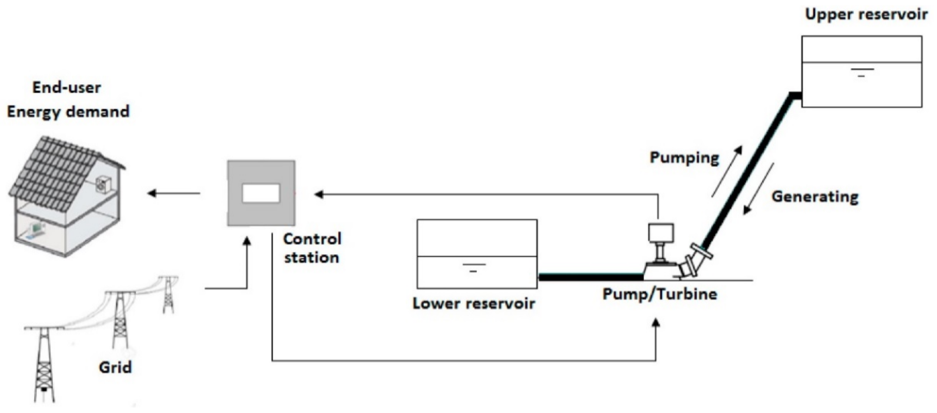
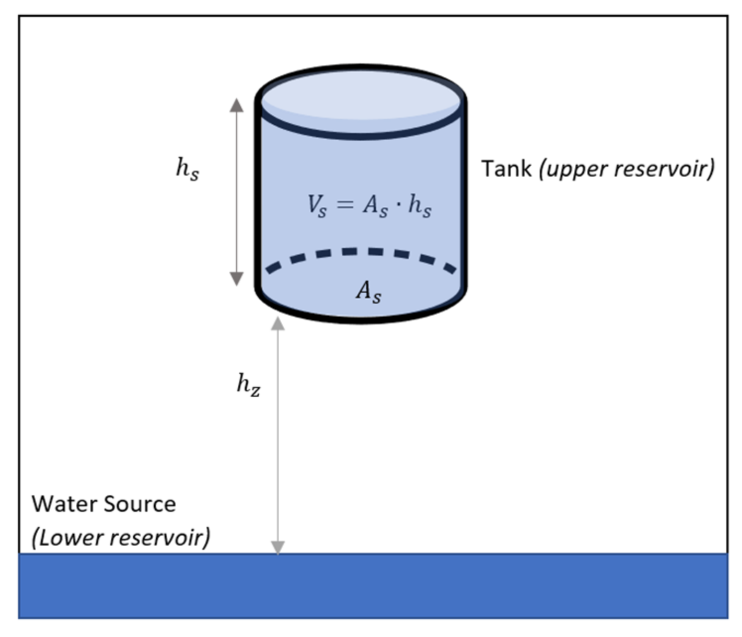
Generally, it can be concluded that pumped hydro storage (PHS) has a relatively high-efficiency range between 70–85% among the long-term ESS and is characterized by a high range of capacities. However, the relatively low energy density of the PHS requires either a large body of water or a large variation in height. For example, 1000 kg of water, i.e., ${1\mathrm{m}}^3$ at the top of a $100\mathrm{m}$ tower has a potential energy of about 0.272 kWh [8]. Therefore, PHS capacity may be practically constrained with limited storage capacity because of their dependency on geographical location. However, despite the geographical challenges, due to the benefits in efficiency, large capacity range, and long possible storage duration, PHS can be considered suitable as a tool to flatten the annual demand curve. Therefore, it is currently the most established technology for controlling energy in the electric power system [7,9].

The authors of [10] have proposed an improved probabilistic production simulation method with a sequential load correction scheme developed to capture the time-dependent features of pumped hydro storage and renewable energy generation. A pumped storage scheduling is used to mitigate the imbalanced power that is caused by the intermittent nature of the distributed energy resources. Hence, the objective function can be defined as the minimization of cumulative imbalanced energy during the scheduling horizon. In Mary, et al. [11], individual scheduling of PHS plants is studied using dynamic programming. The model was tested against two PHS plants placed in IEEE 30 bus system over a 24 h scheduled horizon. As a result, a suitable location for the PSH plants in the system is suggested.

Different modeling strategies have been developed to enhance the capacity to estimate renewable energy. Innovative applications of solar and wind energy as well as the intelligent handling of complicated time-series data signals by neural networks, have both contributed to the forecast of sustainable energy. In order to ascertain whether suggested models can deliver precise estimates of renewable energy output, such as sunlight, wind, or pumped storage, the authors of [12,13] investigate the various information models.

Furthermore, an optimization framework has been presented in Makhdoomi, et al. [14] for the optimal operation of a hybrid system. The system is composed of PV, a diesel generator, and PHS. In Yang, et al. [15], a framework based on reinforced learning is proposed to learn an optimal decision policy for online intelligent economic dispatch. The study was performed on a hybrid hydro/PV/PHS system, considering both the economic benefit and power fluctuation. The authors of [16] have used chaotic fast convergence evolutionary programming (CFCEP) for solving intricate actual world combined heat and power dynamic economic dispatch (CHPDED) problems. The model involved DSM incorporating renewable energy sources and pumped-storage-hydraulic units. In Pali, et al. [17], a concept of small isolated electric power generation from PHS using wind as primary energy is proposed for rural and remote areas. A suitable well is utilized as the lower reservoir of the PHS system, while the upper reservoir (UR) needed for the water storage is made on the ground. The simulated results matched the designed system.

In addition, a medium- to long-term optimal operation strategy is proposed in Liu, et al. [18] for an independent regional power grid in the dry season based on the statistical characteristics of wind–solar power and the long-term plan of hydropower. The objective of the work is to minimize the difference between the monthly water consumption of hydropower stations and the predicted, considering the constraints of water flow and daily average battery energy storage fluctuation. In Wen, et al. [19], the impact of intermittent wind generation, coupled with a given hydro capacity, on wholesale electricity prices, accounting for both spatial and seasonal effects, was investigated. The authors state that during dry seasons, when hydro storage is low and the wind resource is insufficient, relatively more expensive thermal generation is required to satisfy demand, which increases price volatility. In Daneshgar, et al. [20], a solution to help in planning and decision-making for hydropower producers to maximize the profit in the electricity market considering the optimal operation of power plants. A dynamic production profitability model has been developed. The model used in this research leveraged the principles of system dynamics to simulate hydroelectric systems under different scenarios to evaluate the performance of the hydropower generation system. The forecasted profit in each scenario of the hydroelectric plant has been discussed.

Although pumped hydro storage may be seen as a strategic key asset by grid operators and despite the benefits it can add to the grid, financing the PHS project is a concern as it has high investment costs. Therefore, and reference to the reviewed literature, it has been observed that there is a lack of PHS long-term profitability analysis. The more efforts invested in understanding the commercial aspects of PHS, the more guarantees will be established for the payment of the capital cost and a clearer rate of return and hence would motivate the construction of new PHS plants, especially for geographical areas which are not yet identified by the availability of pumped hydro or where it is difficult to find naturally suitable sites close to large water resources with a reasonable height difference between the lower and upper reservoir.

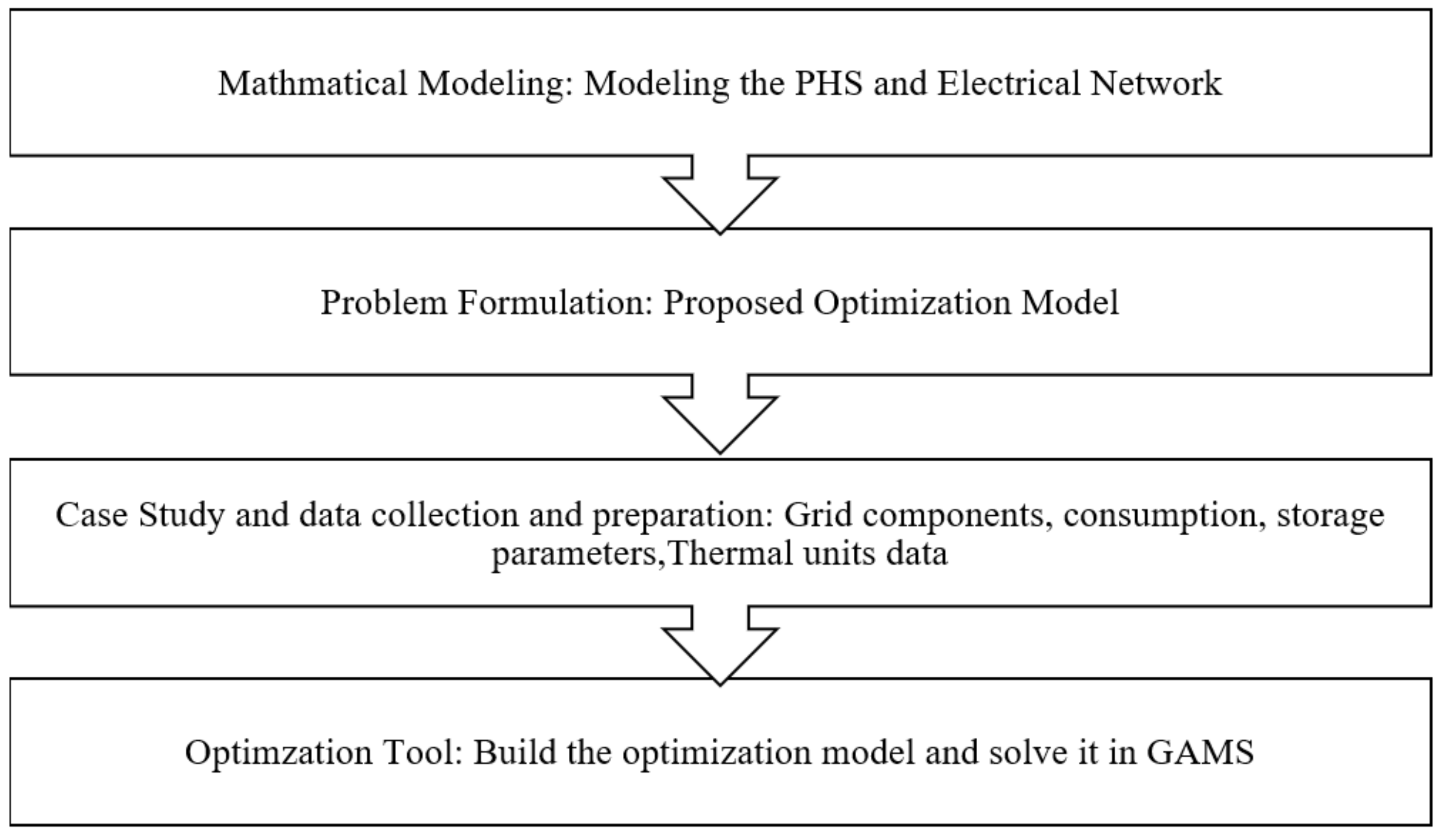
This work proposes a framework to analyze and optimally manage the performance of a seasonal grid-connected PHS unit considering transmission constraints, optimal power flow, and hydraulic model and hydraulic losses, in which it can be adopted for a one-year profitability assessment utilizing GAMS as an optimization tool. Further, the proposed framework is implemented to draw conclusions that would suit the characteristics of the UAE demand pattern, which is identified to be high in seasonal variations. This analysis is essential to motivate the construction of new seasonal PHS plants due to the high construction cost they are identified with, especially in geographical areas where this technology is not yet considered or is hard to construct. The contributions of this work can be summarized as follows:

• Establishing a framework to analyze and optimally manage the seasonal performance of a grid-connected PHS considering transmission constraints, optimal power flow, and hydraulic model and losses.
• Proposing a methodology that can be adopted in assessing the long-term profitability of PHS utilizing GAMS as an optimization tool.
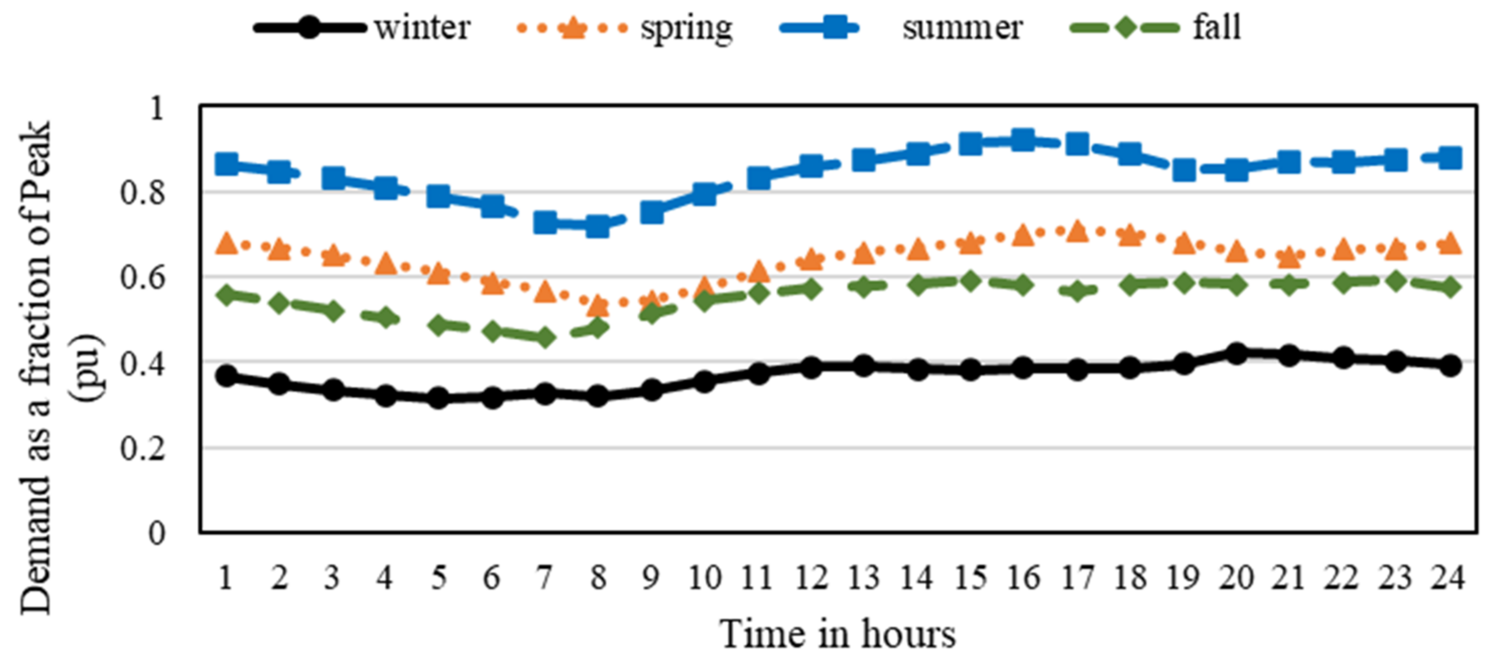
• Implementing the proposed framework to draw conclusions that would suit the characteristics of the UAE demand pattern, which is identified to be high in seasonal variations.

The rest of the paper is organized as follows; Section 2 describes the fundamentals of PHS. The methodology of the proposed approach is presented in Section 3. Section 4 discusses the results and findings. Finally, the work is concluded in Section 5.

2. PHS Fundamentals

This section discusses configurations, elements, power equations, and basic hydraulic terms associated with PHS. Further, Hydro generator types are presented.

2.1. PHS Configuration

PHS is categorized as a closed or open loop based on its connection to flowing water sources. According to the federal energy regulatory commission, closed-loop pumped storage is not permanently connected to a naturally flowing water feature, while open-loop pumped storage is. PHS plants with closed loops are typically limited to daily or weekly storage cycles because being disconnected from a continuous water source implies limited water input into the system [21,22]. There have been three different configurations of PHS: a binary set, a ternary set, and a quaternary set, as explained below [23]:

• Binary set composed of one reversible pump-turbine unit and one electrical machine (motor/generator),
• The ternary set is composed of one turbine, one pump, and one electrical machine (motor/generator), and
• Quaternary set in which one turbine is driving one generator and one motor for one pump.

The earliest PHS in the world appeared in the Alpine regions of Switzerland, Austria, and Italy in the 1890s. The earliest designs used separate pump impellers and turbine generators. Since the 1950s, a single reversible pump turbine has become the dominant design for PHS [24].

2.2. PHS Modeling

The potential energy in joules of a mass $m$ located at the top of a dam is represented by (1) and (2) [25]. Equation (1) can be written in terms of potential energy difference, as shown in (3).

$$\mathrm{P}\mathrm{E}=F\times h,$$

(1)

$$F=m\times g,$$

(2)

$$E_{max}=∆E_{PE}=m\times g\times ∆h,$$

(3)

where $∆h$ is the elevation difference between two points in meters; $F$ is the force or the weight in Newton; $h$ is the height of the mass from a reference point in meters; $m$ is the mass in $\mathrm{k}\mathrm{g}$; $\mathrm{g}$ is the gravitational acceleration in $\mathrm{m}/{\mathrm{s}}^2.$

Dividing (3) by time, we obtain the mass flow rate $\dot{m}$ instead of mass and power instead of energy, as in (4). Further, the mass flow rate can be written in terms of volume flow rate $Q$, where the mass flow rate $\dot{m}$ is equal to the volume flow rate $Q$ multiplied by the total mass density $\rho$ in (4) [26]. Hence, the PHS power equation can be defined as in (5) and (6) [26].

$$\dot{m}=Q\times \rho ,$$

(4)

$$P=Q\times \rho \times g\times ∆h,$$

(5)

$$P=\dot{m}\times g\times ∆h,$$

(6)

However, since we have losses in the system, we do not obtain the total energy or power out; it will be reduced by a certain amount depending on the turbine efficiency ${\eta }_t$. Thus, the total energy in Joules stored in PHS and the output power at a certain head and flow rate are represented in (7) and (8), respectively.

$$E_{stored}={\eta }_t\times \rho \times V\times g\times \mathrm{h}$$

(7)

$$P={\eta }_t\times Q\times \rho \times g\times ∆h$$

(8)

where $E_{stored}$ is the total energy stored in jouls; $\rho$ is water density in $\mathrm{k}\mathrm{g}/{\mathrm{m}}^3$; $V$ represents the volume in ${\mathrm{m}}^3$; $P$ denotes the power in watts; $Q$ the volume flow rate.

2.3. Hydraulic Head

The head is a vital element in the PHS energy storage principle. The hydraulic head measures the amount of mechanical energy per unit weight of the fluid. The difference between the headwater level in the reservoir upstream and the tailwater level in the reservoir downstream determines how much energy can be captured in a PHS planet. From the law of conservation of energy, if we can calculate the energy of a flowing liquid at the start of a pipe system point one, then we know that the same energy must apply at the end of the pipe, point two, even though the values for each form of energy may have altered. If we ignore energy losses, then we are left with potential energy due to height, potential energy due to pressure, and kinetic energy due to motion.

Potential energy due to height is calculated regarding some datum level, such as the ground, as in (1) and represented again in (9) with the symbol $z_1$ instead of $h$. Further, potential energy due to pressure represents the fact that the mass m could rise higher if the pipe were to spring a leak. It would rise by a height of $h_1$, in which $h_1$ is described as $\left(h_1=\frac{P_1}{\rho g}\right)$. The kinetic energy is calculated using (11), where $v$ the water velocity in $\mathrm{m}/\mathrm{s}$. Therefore, the total energy of the mass m at point one can be given in (12).

$${PE}_{height}=mg{z}_1$$

(9)

$${PE}_{pressure}=mg{h}_1$$

(10)

$$KE=\frac{1}{2}m{v}^2$$

(11)

$$E_1=mg{z}_1+mg{h}_1+\frac{1}{2}m{v}_1^2$$

(12)

Similarly, the energy of the same mass at point two can be given by (13). Therefore, by equating (12) and (13), canceling m and dividing by g, we obtain (14).

$$E_2=mg{z}_2+mg{h}_2+\frac{1}{2}m{v}_2^2$$

(13)

$$z_1+h_1+\frac{v_1^2}{2g}=z_2+h_2+\frac{v_2^2}{2g}$$

(14)

This is known as Bernoulli’s equation, after the French scientist who developed it, and is the fundamental equation of hydrodynamics. The dimensions of each of the three terms are the length, and therefore they all have units of meters. For this reason, the third term, representing kinetic energy, is often referred to as the velocity head. The three terms on each side of the equation are sometimes known as the total head. When carrying out calculations using Bernoulli’s equation, it is occasionally helpful to use the substitution $\left(h=\frac{P}{\rho g}\right)$ to change from head to pressure, and it is often helpful to use the substitution $\left(v=\frac{Q}{A}\right)$ because the volume flow rate is the most common way of describing the liquid’s velocity [27]. Figure 1 illustrates Bernoulli’s principle; the sum of pressure (potential energy) and kinetic energy is constant, i.e., energy is conserved if frictional losses are ignored. Thus, when a fluid flows through areas of different diameters, there is a change in velocity, and the change in velocity leads to a change in kinetic energy, so the pressure changes. A decreased pipe diameter means an increase in velocity and kinetic energy and a decrease in pressure [28].

In a pumped hydro storage head is a difference in elevation between the upper and lower water surface levels, which provides the pressure to drive the turbines. Hence, the hydraulic head can be defined as the height of a static water column above a chosen location, often measured in meters. The hydraulic head or water level at a certain site determines how much energy the water there has [29].

The gross head is the physical elevation difference between these two levels. However, when calculating the output of the plant, the net head is used, considering the reduction in pressure due to waterway friction losses and losses at intakes, bends, and changes in the waterway section. Pumped storage schemes are designed to minimize these hydraulic losses, which are typically less than 2% of the gross head. Gross head minus head losses equal the effective or net head as in (15).

$$H_{net}=H_{gross}-H_{loss}$$

(15)

Note that since the PHS depends on a natural water source as a lower reservoir, it is an open loop. This was included to enrich the technical background of the PHS and to clarify that the open loop PHS are more likely to be used as seasonal storage because of the unlimited water supply.

2.4. Hydropower Generator

Hydropower generators can be characterized by fixed and variable speeds. The fixed type is the synchronous generator which is distinguished by a direct grid connection. With this type, hydroelectric or pumped storage installations operate at a constant speed mandated by the synchronous speed of the generator. An induction generator typically experiences a speed variation of 1% to 2%, whereas synchronous generators have no speed variation [30,31]. The second type is the adjustable-speed generator. One common choice of this type of generator is a doubly fed induction generator (DFIG). Figure 2a illustrates the operating point of a constant-at-synchronous-speed hydro turbine, which moves along the dashed line, as the output power is varied by adjusting the wicket gate opening (α). The conversion efficiency of the operating turbine will vary as the output power changes at constant synchronous rotational speed since, for any output power, there will be only a single matching rotational speed that will yield maximum efficiency. On the other hand, the dashed line in Figure 2b illustrates the operating point of variable speed operation, which allows the rotational speed and the wicket gate opening to follow the desired output power. Hence, the operating point of the hydro turbine can follow the maximum efficiency.

3. Methodology

In this section, we present the methodology illustrated in Figure 3. First, we build the mathematical model and formulate the proposed optimization problem. Further, the case study, including data collection, preparation, and assumptions to establish the input to the optimization problem, is presented; this includes consumption data, thermal generation units’ technical data and cost function coefficients, transmission lines power limits, and technical parameters, and PHS unit parameters. Finally, the optimization tool is discussed.

3.1. Network Mathematical Model

This subsection introduces the multi-period mathematical model of the proposed system, the subscript t denotes the time in hours, and the subscript d donates days. The time step$∆T$ is considered as one hour.

3.1.1. PHS Unit Model

PHS system has four main elements: pipes or penstock, the pump, the upper and lower reservoirs, and the hydro turbine. In this section, we present the mathematical model of the four elements.

(A)

Penstock

Pipes or penstock’s primary objective is to convey water as it moves from one point to another. However, while water is transported, its energy is dissipated in pipes due to friction, which is translated into water head losses. Hydraulic head losses are expressed in meters. Several equations in literature are used to describe friction head loss along a pipe. We choose Darcy–Weisbach for this research [32]. The head loss equation is presented in (16), where $R$ is the hydraulic resistance of the pipe, $H_{losses}$ is head loss in $\mathrm{m}$, and $Q$ is the flow in ${\mathrm{m}}^3/\mathrm{s}$.

$$H_{d,t}^{loss}=R{Q}_{d,t}^2,$$

(16)

$$\mathrm{R}=\mathrm{K}·\frac{8}{{\pi }^2·{\mathrm{D}}^4·g},$$

(17)

$$K=K_{pipe}+K_{fitting},$$

(18)

$$K_{pipe}=\frac{f·L_p}{D_p},$$

(19)

$$f=[1.8\log (\frac{6.9}{Re}+(\frac{\raisebox{1ex}{$\epsilon $}\!\left/ \!\raisebox{-1ex}{$D$}\right.}{3.7}{)}^{1.11}{]}^{-2},$$

(20)

$$R_e=\frac{\rho \nu D}{\mu },$$

(21)

$$\nu =\frac{Q}{A},$$

(22)

$$\nu =\frac{\mathrm{Q}}{0.25·\pi ·D^2},$$

(23)

where K represents the total resistance coefficient which consists of the resistance coefficient of the pipe $\left(K_{pipe}\right)$ and resistance coefficient of the pipe fittings $\left(K_{fitting}\right)$. The resistance coefficient of the pipe $\left(K_{pipe}\right)$ is a function of the friction factor $f$ while $\left(K_{fitting}\right)$ depends on the pipe fittings material, and $D$ is the pipe diameter. In addition, $f$ represents the dimensionless Darcy–Weisbach friction factor, which is a function of the Reynolds number, denoted $\left(R_e\right)$ and $\left(\frac{\mathsf{\epsilon }}{\mathrm{D}}\right)$ is the relative roughness, where $\mathsf{\epsilon }$ in $\mathrm{m}\mathrm{m}$ is the absolute roughness, and it depends on the pipe material. The friction factor $f$ in Darcy–Weisbach can be determined from the Moody diagram or by solving the Colebrook-White equation. There are, in the literature, several formulas that approximate the Darcy friction coefficient $f$, we used Equation (20). This equation is derived from the Moody chart to approximately calculate the friction factor $f$. The Reynolds number $\left(R_e\right)$ is a dimensionless number used to categorize the fluids system in terms of the flow pattern of a fluid. Further, $\mu$ is the dynamic viscosity of water, which is a constant $8.90\times {10}^{-4}$ Pa·s at about 25 °C and $\mathsf{\rho }$ is the water density in $\mathrm{K}\mathrm{g}/{\mathrm{m}}^3$ and it is 997 at 25 °C and $\mathsf{\nu }$ is the water velocity in $\mathrm{m}/\mathrm{s}$. Head loss can be calculated using Equation (16) [33]. Equations (17)–(23) are concerned with calculating the hydraulic resistance of the pipe. Practically, the hydraulic resistance value is variable and depends on the friction factor, which is, in turn, a function of the Reynolds number, denoted $R_e$. Reynolds number depends on the velocity of the flow at a specific time. However, the friction losses and Hydraulic resistance were estimated in this research and assumed constant. From the previous equations, it is evident that the hydraulic resistance of the pipe is directly proportional to the pipe length. Hence it is recommended to reduce the vertical and horizontal distance of the penstock.

(B)

Pump model

The pump model calculates the pump flow rate $Q_{d,t}^p$ as a function of electrical power input to the motor driving the pump $P_m$ as given in (24).

$$Q_{d,t}^p=\varphi \left(P_{d,t}^m\right).$$

(24)

For an electrically driven motor, the input power $P_m$ is the total electrical power supplied to the pump system, i.e., to the electrical motor. Output power is the mechanical power at the pump shaft $P_{d,t}^p$ to elevate the water from the lower reservoir to the upper reservoir. The difference between $P_{d,t}^m$ and $P_{d,t}^p$ comes from the motor’s efficiency ${\eta }_m$. The more efficient the motor is, the less power is lost converting from electrical power to mechanical power. The motor efficiency accounts for both the mechanical and electrical losses of the motor, in which ${\eta }_m$ is a function of $P_m$. However, in this research, we consider the motor efficiency constant. Thus, the mechanical power at the pump shaft or output of the motor can be modeled in (25). Further, the pump output flow rate $Q_{d,t}^p$ is a function of the pump power $P_{d,t}^p$ and is represented in (26).

$$P_{d,t}^p=P_{d,t}^m·{\eta }_m,$$

(25)

$$Q_{d,t}^p=\frac{P_{d,t}^p{\eta }_p}{\rho ·g·H_{d,t}^p},$$

(26)

where ${\eta }_p$ is the pump efficiency and is a function of $Q_{d,t}^p$. However, in this research, the ${\eta }_p$ is constant. The pump should be able to provide a pump head at any time step $H_{d,t}^p$ that is not less than the expected hydraulic head losses $H_{d,t}^{loss}$ which is calculated as clarified in the penstock section and the static head $H_{d,t}^s$ which is defined as the total distance from the water surface in the lower reservoir to the water surface in the upper reservoir. Accordingly, the static head changes as the water levels change in both the lower and upper reservoirs. Hence, the total pump delivered head $H_{d,t}^p$ modeled as in (27). According to (16), pump head loss$H_{d,t}^{p,loss}$ can be modeled as (28).

$$H_{d,t}^p=H_{d,\mathrm{t}}^s+H_{d,t}^{p,loss},$$

(27)

$$H_{d,t}^{p,loss}=R{Q_{d,t}^p}^2,$$

(28)

$$H_{d,t}^s=h_z+l_{d,t-1}.$$

(29)

In this research, the lower reservoir is assumed a natural water source with a fixed level, and the upper reservoir (UR) is a human-made tank with a variable level. Thus, $H_{d,t}^s$ consists of fixed and variable parts since there is a fixed vertical distance between the two reservoirs and the variable part is because the UR water level changes as the tank is being filled or emptied. $H_{d,t}^s$ can be hence calculated as in Equation (29), where $h_z$ is the fixed vertical elevation between the two reservoirs and $l_{d,t-1}$ is the water level in the UR before pumping occurs; therefore, time subscript is reduced by 1.

(C)

UR model

The UR model represents dynamic modeling of the water level in the reservoir due to the increment or decrement during the pump or turbine operation and can be represented as in (30).

$$l_{d,t}=l_{d,t-1}+\left(\frac{Q_{d,t}^p-Q_{d,t}^{tur}}{A}\right)·∆T,$$

(30)

where $Q_{d,t}^{tur}$ is the turbine flow rate in case of discharging and $Q_{d,t}^p$ is the pump flow rate in case of charging. $A$ is the cross-sectional area in ${\mathrm{m}}^2$ of the tank, $l_{d,t-1}$ is the previous level of the tank and $∆T$ is the time interval in hours.

(D)

Turbine model

The turbine model calculates the turbine output power $P_{d,t}^{tur}$ as a function of the flow rate $Q_{d,t}^{tur}$ and the turbine head $H_{d,t}^{tur}$ and given in (31) and (32).

$$P_{d,t}^{tur}=\varphi \left(Q_{d,t}^{tur},H_{d,t}^{tur}\right),$$

(31)

$$P_{d,t}^{tur}=n_t·\rho ·Q_{d,t}^{tur}·g·H_{d,t}^{tur}.$$

(32)

In reverse to the pump operation, the mechanical energy is converted into electrical energy. The efficiency of the turbine $n_t$ reflect how much energy is lost due to mechanical losses in the turbine and how much is converted into electrical energy, and it is a function of a turbine flow [33]. However, in this research, the turbine efficiency is assumed constant, where $H_{d,t}^{tur}$ is the net head driving the turbine at specific time step. Net head is defined as the actual water pressure driving the turbine after deduction of friction losses in the waterway but adding back the kinetic energy of the water flow based on the explained Bernoulli principle previously. Mathematically, the net head can be presented as a gross static head minus the head losses. In this study, we are assuming the turbine to be a Francis turbine type which can operate in either pumping or turbine mode, in which gross static head is defined as the distance from the water surface in the lower reservoir to the water surface in the UR which is the same definition of the static head in the previous section $H_{d,t}^s$. Hence, the turbine net head $H_{d,t}^{tur}$ equal static head minus the head loss $H_{losses,t}$ along the penstock (33). Reference to (16), turbine head loss $H_{d,t}^{t,loss}$ can be modeled in (34).

$$H_{d,t}^{tur}=H_{d,t}^s-H_{d,t}^{t,loss},$$

(33)

$$H_{d,t}^{t,loss}=R{Q_{d,t}^{tur}}^2.$$

(34)

3.1.2. DC power flow model

In order to construct a DC power flow model, the below assumptions have to be considered:

• Line resistances (active power losses) are negligible, i.e., $\mathrm{R}\ll \mathrm{X}$.
• Voltage angle differences are assumed to be small, i.e., $\mathit{sin}\theta =\theta$ and $\mathit{cos}\theta =1$.
• Magnitudes of bus voltages are set to 1.0 per unit (flat voltage profile).

It is worth mentioning that DC power flow is a variation of the Newton–Raphson method; hence, reflecting the above assumptions, Equation (35) which represents AC active power flow used in Newton–Raphson method, can be reduced to Equation (36) resulting in a formulation between P and θ. Hence, voltage angles and active power injections are the variables of the DC power flow problem. Equations (36)–(38) reflect the assumptions mentioned above, respectively, where $P_i$ is the injected power at bus i, in which $B_{ij}$ is susceptance of the transmission line. Any given transmission circuit with an impedance of $Z=R+jX$, will have an admittance of $Y=G+jB$. Since the line resistances (active power losses) are negligible, $B_{ij}$ will be the reciprocal of the reactance $X_{ij}$ between bus i and bus j. As a result, active power flow through a transmission line between buses i and j at time t and day d can be formulated in (39), where $X_{d,t}^{ij}$ is the reactance of line ij, ${\theta }_{d,t}^i-{\theta }_{d,t}^j$ is Voltage angle differences and $P_{d,t}^{ij}$ is the power flow between buses i and j.

$$P_i=\left|V_i\right|\sum _{j=1}^n\left|V_j\right|[G_{ij}\mathit{cos}\left({\theta }_i-{\theta }_j\right)+B_{ij}·\mathit{sin}({\theta }_i-{\theta }_j),$$

(35)

$$P_i=\sum _{j=1}^n{B}_{ij}·sin\left({\theta }_i-{\theta }_j\right),$$

(36)

$$sin\left({\theta }_k-{\theta }_i\right)=\left({\theta }_k-{\theta }_i\right),$$

(37)

$$P_i=\sum _{j=1}^n\left[B_{ij}·\left({\theta }_i-{\theta }_j\right)\right],$$

(38)

$$P_{d,t}^{ij}=\frac{{\theta }_{d,t}^i-{\theta }_{d,t}^j}{X_{d,t}^{ij}}.$$

(39)

3.1.3. Dynamic Economic Dispatch (DED)

In this research, a cost-based DED problem as a convex cost function is used for simplicity [34]. The production costs of a thermal unit are defined in Equation (40) where $a_g$, $b_g$, and $c_g$ are the fuel cost coefficients of the $jth$ unit.

$$Cost=\sum _g{a}_g{\left(P_{d,t}^g\right)}^2+b_g\left(P_{d,t}^g\right)+c_g.$$

(40)

This research only considers coupling in the time domain through ramp rates constraints Equations (41) and (42). Ramp rates state what is the maximum possible change in a unit output over a period, where $R{U}_g$ represents the upper ramp rate limit of generators when generation must be increased due to an increase in load and $R{D}_g$ represents down ramp rate limit of generators when generation must decrease due to a decrease in load, $P_{g,t}$ is the current generation of the unit and $P_{g,t-1}$ is the previous generation of the unit [35]. In addition, the operational constraints on the thermal units are given in where $P_g^{min}$ is the minimum Active power generated by thermal unit and $P_g^{max}$ (43).

$$P_{d,t}^g-P_{d,t-1}^g\le R{U}_g,$$

(41)

$$P_{d,t-1}^g-P_{d,t}^g\le R{D}_g,$$

(42)

$$P_g^{min}\le P_{d,t}^g\le P_g^{max}.$$

(43)

3.1.4. Problem Formulation

In this section, we formulate the proposed optimization problem, which combines the network power flow, DED, and PHS unit.

• Objective function:

The objective function is the DED thermal generation units cost function, except it will be multiplied by 90 to account for the full season as in (45); a detailed explanation for the study period is in the next Section 3.2 under Study period and demand data. The operation cost should be minimized over the study period, where $g$is the index of thermal generating units. The real power output of the corresponding thermal generator units and the PHS unit represents the decision variables and are optimized according to the objective. An illustration of the proposed system configuration is presented in Figure 4. The decision variable vector $P_{d,t}^{gen}$ is represented in (44) where n is the number of the thermal units to be scheduled within the network, i.e., the 12 in addition to ($P_{d,t}^p$) and ($P_{d,t}^{tur})$ related to the BHS unit.

$$P_{d,t}^{gen}=[\begin{array}{ccc}{P}_{d,t}^1& P_{d,t}^n& \dots \end{array} P_{d,t}^n P_{d,t}^p P_{d,t}^{tur}{]}^T.$$

(44)

$$\min (\mathrm{C}\mathrm{o}\mathrm{s}\mathrm{t})=\sum _{\mathrm{d},\mathrm{t},\mathrm{g}}90\times \left\{{\mathrm{a}}_{\mathrm{g}}{\left({\mathrm{P}}_{\mathrm{d},\mathrm{t}}^{\mathrm{g}}\right)}^2+{\mathrm{b}}_{\mathrm{g}}\left({\mathrm{P}}_{\mathrm{d},\mathrm{t}}^{\mathrm{g}}\right)+{\mathrm{c}}_{\mathrm{g}}\right\}.$$

(45)

• Equality constraint

  -

  Power balance equation is constructed by equating (39) and the left-hand side of (46); this implies that the power balance between generation, demand, and power transfers should be satisfied in all time steps. Noting that $P_{d,t}^{tur}$ and $P_{d,t}^p$ are with positive and negative signs, respectively, to reflect the charging and discharging of PHS units,

  $$\sum _{g\in {\mathsf{\Omega }}_G^i}{P}_{d,t}^g+P_{d,t}^{tur}-P_{d,t}^p-P_{d,t}^d=\sum _{j\in {\mathsf{\Omega }}_l^i}{P}_{d,t}^{ij},$$

  (46)

  where $j$ and $i$ are the indexes of network buses; ${\mathsf{\Omega }}_g$ is the set of all thermal generating units; ${\mathsf{\Omega }}_G^i$ is the set of all thermal generation units connected to bus $i$; ${\mathsf{\Omega }}_l$ is the set of network branches; ${\mathsf{\Omega }}_l^i$ represents the set of all busses connected to bus $i$; $P_{d,t}^d$ denotes the demand.

  -

  Pump and turbine power Equations (25) and (32),

  -

  Pump and turbine head Equations (27) and (33),

  -

  Pump and turbine head loss Equations (28) and (34),

  -

  The water level in the UR Equation (30), and

  -

  UR initial value at the beginning of each season (47)–(50).

In addition to the equality constraints on the water level in the upper reservoir, four more equations are included in the model to link the initial values in the UR at the beginning of each season to the previous season. Each season is approximated as one day. Therefore, the difference between the water level in the last hour, i.e., 24 from a specific day representing a specific season, and the initial value of the same day multiplied by 90 and added to the initial value of the same day should be equal to the initial value of the UR level of the next day, i.e., season.

$$l_2^i=l_1^i+90\times \left({l_{1,24}-l}_1^i\right),$$

(47)

$$l_3^i=l_2^i+90\times \left({l_{2,24}-l}_2^i\right),$$

(48)

$$l_4^i=l_3^i+90\times \left({l_{3,24}-l}_3^i\right),$$

(49)

$$l_1^i=l_4^i+90\times \left({l_{4,24}-l}_4^i\right).$$

(50)

• Inequality constraints

  -

  Ramp-up and ramp-down constraints are represented in (41) and (42),

  -

  Thermal units operating limits in Equation (43),

  -

  Network transmission line limits in Equation (51),

  -

  Pump and Turbine power limits in (52) and (53),

  -

  Flow minimum limits: however, maximum limits are constrained with the pump and turbine maximum power limits (54) and (55),

  -

  UR maximum and minimum level limits (56),

  -

  UR initial value maximum and minimum level limits (57), and

  -

  Voltage angle limits (58).

$${-P}_{ij}^{max}\le P_{d,t}^{ij}\le P_{ij}^{max},$$

(51)

$$P_{d,t}^{min}\le P_{d,t}^{tur}\le P_{d,t}^{max},$$

(52)

$$P_{d,t}^{min}\le P_{d,t}^p\le P_{d,t}^{max},$$

(53)

$$Q_{d,t}^{t,min}\le Q_{d,t}^t,$$

(54)

$$Q_{d,t}^{p,min}\le Q_{d,t}^p,$$

(55)

$$l_{d,t}^{min}\le l_{d,t}\le l_{d,t}^{max},$$

(56)

$$l_{d,t}^{min}\le l_d^i\le l_{d,t}^{max},$$

(57)

$${\mathsf{\theta }}_{d,t}^{min}\le {\mathsf{\theta }}_{d,t}^i\le {\mathsf{\theta }}_{d,t}^{max},$$

(58)

where $l_d^i$ and $l_{d,t}$ are the initial and current levels of the upper reservoir, respectively. $Q_{d,t}^p$ represents the pumping flow. $P_{d,t}^{ij}$ and ${\mathsf{\theta }}_{d,t}^i$ are the power flow in line $ij$ and voltage angle, respectively.

3.2. Case Study: Data Collection and Preparation

Here, the data and assumptions considered in this research are presented.

3.2.1. Study Period and Demand Data

PHS performance is expected to vary throughout the year due to seasonal variations in electricity demand. Hence, the study period of one year was considered to monitor the effect of seasonal variation on charging and discharging decisions with a time step of one hour. A one-year demand figure was retrieved from Sharjah Electricity, water, and gas authority (SEWA) and divided into four quarters, each of approximately 90 days, in which each quarter represents a season. Hence, the average demand of the same hour of each day in the same season was calculated, i.e., we ended up with demand data for 4 days and 96-time steps. This representation of the study period is performed to ensure a manageable simulation time.

3.2.2. Test System

This research utilizes the IEEE 24-bus Reliability Test System (RTS), a transmission network with voltage levels of 138 kV and 230 kV, and base demand is 100 MVA. The Electrical network is shown in Figure 5. The system is modified to integrate a PHS unit at bus 19, as shown in the figure. The network is structured using the transmission lines’ power limits, and technical parameters, using the generating units’ data and connection details, as retrieved from ref. [34], with modifications. There are 12 thermal generating units connected to different buses, in which the sum of the maximum possible output of all units is 3375 MW. The slack bus is chosen to be bus 13. The maximum possible demand for all buses is, at most, 2850 MW. The values of all coefficients of thermal generating units utilized to calculate the variables are given in

Table A1. Thermal Generating units’ data.

Gen	Bus	${\mathit{P}}_{\mathit{i}}^{\mathit{m}\mathit{a}\mathit{x}}\mathbf{M}\mathbf{W}$	${\mathit{P}}_{\mathit{i}}^{\mathit{m}\mathit{i}\mathit{n}}\mathbf{M}\mathbf{W}$	${\mathit{a}}_{\mathit{i}}$$(\mathbf{USD}/{\mathbf{M}\mathbf{W}}^2)$	${\mathit{b}}_{\mathit{i}}$$(\mathbf{USD}/\mathbf{M}\mathbf{W})$	${\mathit{c}}_{\mathit{i}}$$\left(\mathbf{USD}\right)$	RU (MW/h)	RD (MW/h)
g1	18	400	90	117.7	5.47	0.02533	47	47
g2	21	420	100	117.7	5.47	0.01199	47	47
g3	1	152	30.4	100	13.32	0.005	14	14
g4	2	152	30.4	660	13.32	0.00413	14	14
g5	15	155	54.25	300	16	0.0025	21	21
g6	16	155	54.25	81	10.52	0.00876	21	21
g7	23	310	108.5	500	10.52	0.002	21	21
g8	23	350	140	500	10.89	0.00623	28	28
g9	7	350	75	217	20.7	0.00211	49	49
g10	13	591	206.85	680	20.93	0.02533	21	21
g11	15	60	12	680	26.11	0.01199	7	7
g12	22	300	0	100	26	0.005	35	35

(Appendix A).

3.2.3. PHS Unit Assumptions and Parameters

This section presents the technical parameters and assumptions considered for the PHS. This research assumes that the PHS configuration is a one-unit configuration hosted in a powerhouse, a reversible pump turbine coupled to a reversible motor generator. The parameters considered for both modes can be discussed as follows,

(A)

Lower reservoir

A lower reservoir is assumed to be a water source at sea level, with a fixed water level acting as a reference point to the system.

(B)

Upper reservoirs

The UR is assumed to be above the lower reservoir by $h_z$ equal to $210 \mathrm{m}$, the assumed cross-sectional area $A_s$ is 25,510 m², and the reservoir height $h_s$ is $90 \mathrm{m}.$ Previously defined (7) can be used to calculate the storage volume $V_s$ assuming the tank has a cylindrical shape and substituting the total head $h_t$ and the desired storage capacity. Equations (59) and (60) define $h_t$ and $A_s$ the cross-sectional area of the upper reservoir. Figure 6 shows a graphical illustration of storage parameters.

$$h_t=h_s+h_z,$$

(59)

$$A_s=\frac{V_s}{h_s}.$$

(60)

(C)

Storage cycle

Since the proposed PHS unit is intended to be simulated as seasonal storage, the unit is expected to store and reach the rated storage capacity, i.e., operate in pumping mode in the lower demand seasons. On the other hand, it is assumed that the storage will be fully discharged in the highest-demand seasons. i.e., operate in turbine mode to support the grid. Accordingly, $P_{d,t}^p$ and $P_{d,t}^{tur}$ limits should take into consideration the assumed generation capacity and storage capacity. Substituting in (61), we calculate the required maximum power limits $P_{d,t}^{max}$ for both modes, where ${Cycle}_D$ is the daily assumed discharging cycle duration in hours $E_s^{max}$, is the maximum energy storage capacity, and ${Days}_D$ is the number of days the discharge is expected to occur. On the other hand, the minimum power limit on $P_{d,t}^{min}$ is considered zero.

$$P_{d,t}^{max}=\frac{E_s^{max}}{{Cycle}_D·{Days}_D}.$$

(61)

Table 2. The assumptions for charging and discharging capacities.

Index	Charging	Discharging
Daily hours	6	6
Number of seasons	3	1
Days	270	90

summarizes the assumptions considered for calculating charging and discharging capacities. The charging shall happen for 270 days, 3 seasons at 6 h daily, and the discharging shall happen for 90 days, 1 season at 6 h daily.

(D)

Penstock

The total length of penstock connecting the lower reservoir to the UR is assumed 490 m. A few fittings are considered in the study, and the total $K_{fitting}$ is assumed to be around 10. Penstock diameter can be calculated from Equations (62) and (63). The velocity is assumed to be kept at 5 m/s. Taking a perfect discharging cycle, the maximum flow should happen in turbine mode when rated power is supplied and when the storage is at its lowest level before it is empty. The maximum flow value will not exceed the flow calculated using (64). Substituting the maximum expected flow rate and the assumed velocity, the diameter was found.

$$A_s=0.25\pi D^2,$$

(62)

$$\nu =\frac{Q_{d,t}^{max}}{A_s},$$

(63)

$$Q_{d,t}^{max}=\frac{P_{d,t}^{max}}{n_t·\rho ·g·h_z}.$$

(64)

The model assumes one penstock for both pumping and turbine mode; hence, the maximum flow to calculate the pipe diameter will be considered from turbine mode since it is higher. Penstock technical parameters are summarized in

Table 3. The penstock technical parameters.

Penstock Material	Carbon Steel
Absolute roughness $\epsilon$in mm	0.3 mm
Relative roughness $\raisebox{1ex}{$\epsilon $}\!\left/ \!\raisebox{-1ex}{$D$}\right.$	0.00014851
Diameter	In m	In mm
	2.02	2020
Cross-sectional area	3.2 ${\mathrm{m}}^2$
Length	$490\mathrm{m}$

.

3.3. Optimization Tool

The formulated optimization problem is built and solved in GAMS, a General Algebraic Modeling System for mathematical optimization and simulations using The Branch-And-Reduce Optimization Navigator solver (BARON). BARON solves nonlinear (NLP) problems globally. The branch-and-bound deterministic global optimization algorithms of the type used in BARON are guaranteed to generate global optima under reasonably generic assumptions; these include the presence of finite lower and upper bounds [36].

4. Results and Discussions

In this section, the simulation results and evaluation of the performance of the proposed network are presented. Simulations aim to evaluate the three aspects of the proposed network:

• Peak shaving effect; through reflecting the difference in the operation of expensive thermal units before and after PHS unit integration,
• Charging and discharging decisions as a response to seasonal demand variation, and
• Cost of operation.

4.1. Peak Shaving Affect

The peak shaving effect is demonstrated by testing the network with and without PHS. The storage capacity considered in this simulation is 1500 MWh. However, it is to be noted that during this comparison, the optimal power flow (OPF) is obtained for the network based on the optimization problem formulated in the previous section, except that no RU and RD constraints and thermal unit lower limits were reduced to zero to be able to observe the contribution of the storage on the reduction of expensive power plants operation without the effect of other constraints. Figure 7 presents the difference in energy production per year for each unit, where negative values indicate a reduction, whereas positive values indicate an increment (peak shaving and valley filling). The total increase and reduction of the unit’s production are 1791 MWh/year and 1512 MWh/year, respectively. Further, to observe the reduction or increment based on each unit cost, Figure 8 is used to illustrate the generation cost for the thermal units per MWh.

4.2. Charging and Discharging of the PHS

In order to observe the performance of charging and discharging decisions as a response to seasonal demand variations, the average hourly demand for each season in UAE is presented in Figure 9, and the water level of the UR is plotted against the whole year with a one-hour time interval in Figure 10 (Note that each color code represents a season). Further, the proposed PHS was simulated with different charging and discharging (generation) capacities, i.e., lower and higher than the proposed storage cycle capacities. Figure 11 represents the UR level with the increased capacity. In contrast, the plot in Figure 12 is for the reduced capacity. The seasons’ sequence on all UR plots is fall, winter, spring, and summer and is differentiated by colors matching Figure 9 of the average hourly seasonal demand. The PHS unit parameters considered in the comparison in this subsection are presented in

Table 4. The parameters of PHS.

Storage Capacity	Storage Parameters
$1500\mathrm{M}\mathrm{W}\mathrm{h}$	$h_s$	$h_z$	$A$
	$90\mathrm{m}$	$210\mathrm{m}$	$\mathrm{25,510}{\mathrm{m}}^2$

.

4.3. Cost of Operation

Generally, the cost of operation encountered reduction due to the peak shaving imposed by the PHS unit. The cost of operation without PHS is 7181 M USD/year; the cost of operation with PHS and annual reduction are presented in

Table 5. Operation cost with different PHS unit storage capacities.

PHS Capacity	Operation Cost	Cost reduction M USD/Year
200 MWh	7180	0.98
1500 MWh	7179	2.6
15,000 MWh	7159	22.56

for different storage capacities. On the other hand,

Table 6. Operation cost increasing charging and discharging capacities.

PHS Capacity	Operation Cost USD	Cost reduction M USD/Year
1500 MWh	7176	5.5

presents the reduction in operation cost between the 1500 MWh PHS of the proposed and increased charging and discharging capacities.

4.4. Performance Evaluation

The results demonstrated that the proposed model successfully simulates the grid-connected PHS’s seasonal performance. This was verified by demonstrating the peak shaving effect, the UR level graphs, and the reduction in the operation cost. The reduction in annual energy production from certain thermal units in the presence of 1500 MWh PHS unit reached approximately 1512 MWh annually, of which 1224 MWh is from the expensive thermal units; hence, it is a good contribution to peak shaving. Further, though unit g6 is the cheapest unit, it did not produce more energy after integrating the PHS unit because it operates at its maximum limit in both cases. Further, the energy reduction from thermal units is less than the increment due to the system efficiency; the total increment was 1791 MWh, while the total reduction was 1512 MWh. On the other hand, the UR level plots demonstrated that most pumping occurs in the lowest demand season, winter. In contrast, the water level is almost stable in the moderate demand ones, fall, and spring, and then it is fully emptied to support the grid in summer’s highest demand season. However, depending on the charging and discharging capacities, the PHS may tend to charge during fall or spring, as shown in Figure 11, to ensure optimum utilization of surplus power prior to the highest demand season. On the other hand, if charging and discharging capacities are big enough, it may operate to support the grid daily, along with being a seasonal PHS. This is demonstrated in Figure 12 and can be easily spotted from the fluctuations observed in the plot. However, this indicates that daily charging and discharging are essential to optimizing the cost; however, knowing the yearly demand trends from the beginning affects the charging and discharging decisions. If they are only a day ahead, the data are predicted or inputted into the optimization problem. Further, the operation cost obtained for different storage capacities reduced as the storage capacities increased. It is also noticed that increasing the charging and discharging capacities may further reduce the operation cost as the storage charge and discharge daily supports the grid.

5. Conclusions

This research proposed a framework to manage and analyze a grid-connected PHS unit optimally. The proposed framework was deployed to study the seasonal performance of PHS in supporting the grid in the UAE over a study period of one year. The model in this study considers transmission constraints, optimal power flow, and hydraulic model and losses. However, it ignores transmission losses and reactive power. The effectiveness of the proposed framework in simulating the performance of the seasonal PHS unit was demonstrated through several tests to observe the peak shaving effect, the charging and discharging decision as a response to seasonal demand variations, and the operation cost. It was observed that integrating 1500 MWh PHS reduced the operation of expensive thermal units by 1224 MWh annually, and it was evaluated as a good contribution to peak shaving. The UR plots showed that charging mainly occurred in winter, the lowest demand season, whereas discharging was always in the highest demand season, summer. It was concluded that knowing the seasonal trends from an early stage would highly affect the charging and discharging decisions. Further, a reduction in operation cost was recorded after integrating PHS units that ranged from 2.6 M to 22 M USD/year, depending on the storage capacity. Therefore, a trade-off between increasing the construction cost to enlarge the size of PHS and the economic benefits this PHS may contribute should be considered. Further, having an effective seasonal PHS implies that the storage capacity should be sufficient to support the grid on a seasonal basis since a daily PHS plant cannot store energy seasonally. The larger the size of the upper reservoir, the more storage cycles it can perform. The capacity of the PHS unit depends on the water storage capacity of the upper reservoir, the height difference between the upper and lower reservoirs, and the water availability in the lower reservoir.

References

1. Uddin, M.; Romlie, M.F.; Abdullah, M.F.; Abd Halim, S.; Abu Bakar, A.H.; Chia Kwang, T. A Review on Peak Load Shaving Strategies. Renew. Sustain. Energy Rev. 2018, 82, 3323–3332. [Google Scholar] [CrossRef]
2. Salehi Dobakhshari, S.; Milimonfared, J.; Taheri, M.; Moradisizkoohi, H. A Quasi-Resonant Current-Fed Converter with Minimum Switching Losses. IEEE Trans. Power Electron. 2017, 32, 353–362. [Google Scholar] [CrossRef]
3. Shaheen, A.M.; Hamida, M.A.; El-Sehiemy, R.A.; Elattar, E.E. Optimal Parameter Identification of Linear and Non-Linear Models for Li-Ion Battery Cells. Energy Rep. 2021, 7, 7170–7185. [Google Scholar] [CrossRef]
4. Hamida, M.A.; El-Sehiemy, R.A.; Ginidi, A.R.; Elattar, E.; Shaheen, A.M. Parameter Identification and State of Charge Estimation of Li-Ion Batteries Used in Electric Vehicles Using Artificial Hummingbird Optimizer. J. Energy Storage 2022, 51, 104535. [Google Scholar] [CrossRef]
5. El-Sehiemy, R.; Hamida, M.A.; Elattar, E.; Shaheen, A.; Ginidi, A. Nonlinear Dynamic Model for Parameter Estimation of Li-Ion Batteries Using Supply–Demand Algorithm. Energies 2022, 15, 4556. [Google Scholar] [CrossRef]
6. Abou El-Ela, A.A.; El-Sehiemy, R.A.; Shaheen, A.M.; Wahbi, W.A.; Mouwafi, M.T. A Multi-Objective Equilibrium Optimization for Optimal Allocation of Batteries in Distribution Systems with Lifetime Maximization. J. Energy Storage 2022, 55, 105795. [Google Scholar] [CrossRef]
7. Beardsall, J.C.; Gould, C.A.; Al-Tai, M. Energy Storage Systems: A Review of the Technology and Its Application in Power Systems. In Proceedings of the 2015 50th International Universities Power Engineering Conference (UPEC), Stoke on Trent, UK, 1–4 September 2015. [Google Scholar] [CrossRef]
8. Notton, G.; Lazarov, V.; Stoyanov, L. Analysis of Pumped Hydroelectric Storage for a Wind/PV System for Grid Integration. Environ. Eng. Environ. Prot. 2011, 1, 64–74. [Google Scholar]
9. Díaz-González, F.; Sumper, A.; Gomis-Bellmunt, O.; Villafáfila-Robles, R. A Review of Energy Storage Technologies for Wind Power Applications. Renew. Sustain. Energy Rev. 2012, 16, 2154–2171. [Google Scholar] [CrossRef]
10. Zhou, B.; Liu, S.; Lu, S.; Cao, X.; Zhao, W. Cost–Benefit Analysis of Pumped Hydro Storage Using Improved Probabilistic Production Simulation Method. J. Eng. 2017, 2017, 2146–2151. [Google Scholar] [CrossRef]
11. Mary, P.T.; Ram Jethmalani, C.H.; Simon, S.P. Thermal Unit Commitment Considering Pumped Storage Hydro Electricity Plants. In Proceedings of the 2013 International Conference on Energy Efficient Technologies for Sustainability, Nagercoil, India, 10–12 April 2013; pp. 964–969. [Google Scholar] [CrossRef]
12. Alqahtani, A.S.; Kshirsagar, P.R.; Manoharan, H.; Balachandran, P.K.; Yogesh, C.K.; Selvarajan, S. Prophetic Energy Assessment with Smart Implements in Hydroelectricity Entities Using Artificial Intelligence Algorithm. Int. Trans. Electr. Energy Syst. 2022, 2022, 2376353. [Google Scholar] [CrossRef]
13. Krishnamoorthy, M.; Natarajan, K.; Balachandran, P.K.; Srinivasan, S. Design and Simulation of a Renewable-Based Sustainable Electrification System for a Water Purification Plant. In Green Energy Systems: Design, Modelling, Synthesis and Applications; Elsevier: Amsterdam, The Netherlands, 2022; pp. 25–36. ISBN 9780323951081. [Google Scholar]
14. Makhdoomi, S.; Askarzadeh, A. Optimizing Operation of a Photovoltaic/Diesel Generator Hybrid Energy System with Pumped Hydro Storage by a Modified Crow Search Algorithm. J. Energy Storage 2020, 27, 101040. [Google Scholar] [CrossRef]
15. Yang, J.; Zhang, S.; Liu, J.; Han, X.; Peng, W.; Liu, J. Dynamic Dispatch of Hybrid Hydro/PV/PHS Complementary Power Generation System Based on Deep Reinforcement Learning. In Proceedings of the 2021 IEEE 5th Conference on Energy Internet and Energy System Integration (EI2), Taiyuan, China, 22–24 October 2021; pp. 2125–2129. [Google Scholar] [CrossRef]
16. Basu, M. Combined Heat and Power Dynamic Economic Dispatch with Demand Side Management Incorporating Renewable Energy Sources and Pumped Hydro Energy Storage. IET Gener. Transm. Distrib. 2019, 13, 3771–3781. [Google Scholar] [CrossRef]
17. Pali, B.S.; Vadhera, S. A Novel Pumped Hydro-Energy Storage Scheme with Wind Energy for Power Generation at Constant Voltage in Rural Areas. Renew. Energy 2018, 127, 802–810. [Google Scholar] [CrossRef]
18. Liu, Z.; Zhang, Z.; Zhuo, R.; Wang, X. Optimal Operation of Independent Regional Power Grid with Multiple Wind-Solar-Hydro-Battery Power. Appl. Energy 2019, 235, 1541–1550. [Google Scholar] [CrossRef]
19. Wen, L.; Suomalainen, K.; Sharp, B.; Yi, M.; Sheng, M.S. Impact of Wind-Hydro Dynamics on Electricity Price: A Seasonal Spatial Econometric Analysis. Energy 2022, 238, 122076. [Google Scholar] [CrossRef]
20. Daneshgar, S.; Zahedi, R. Investigating the Hydropower Plants Production and Profitability Using System Dynamics Approach. J. Energy Storage 2022, 46, 103919. [Google Scholar] [CrossRef]
21. ESA. Surface Reservoir Pumped Hydroelectric Storage. Available online: https://energystorage.org/why-energy-storage/technologies/surface-reservoir-pumped-hydroelectric-storage/ (accessed on 1 February 2023).
22. Hunt, J.D.; Zakeri, B.; Nascimento, A.; Brandão, R. Pumped Hydro Storage (PHS). In Storing Energy, 2nd ed.; with Special Reference to Renewable Energy Sources; Elsevier: Amsterdam, The Netherlands, 2022; pp. 37–65. [Google Scholar] [CrossRef]
23. Bitew, G.T.; Han, M.; Mekonnen, S.A.; Patrobers, S.; Khan, Z.W.; Tuan, L.K. Pumped Energy Storage System Technology and Its AC–DC Interface Topology, Modelling and Control Analysis: A Review. J. Eng. 2019, 2019, 705–710. [Google Scholar] [CrossRef]
24. Rehman, S.; Al-Hadhrami, L.M.; Alam, M.M. Pumped Hydro Energy Storage System: A Technological Review. Renew. Sustain. Energy Rev. 2015, 44, 586–598. [Google Scholar] [CrossRef]
25. Murray, R.L.; Holbert, K.E. Energy. In Nuclear Energy; Elsevier: Amsterdam, The Netherlands, 2020; pp. 3–13. [Google Scholar]
26. Tosun, I. Steady Microscopic Balances with Generation. In Modeling in Transport Phenomena; Elsevier Science B.V.: Amsterdam, The Netherlands, 2007; pp. 305–407. ISBN 978-0-444-53021-9. [Google Scholar]
27. Gentle, R.; Edwards, P.; Bolton, B. Fluid Mechanics. In Mechanical Engineering Systems; Butterworth-Heinemann: Oxford, UK, 2001; pp. 112–168. ISBN 978-0-7506-5213-1. [Google Scholar]
28. Bajpai, P. Biermann’s Handbook of Pulp and Paper; Elsevier: Amsterdam, The Netherlands, 2018. [Google Scholar]
29. Hydraulic Head—Energy Education. Available online: https://energyeducation.ca/encyclopedia/Hydraulic_head#cite_note-RE1-2 (accessed on 31 January 2023).
30. Kerkman, R.J.; Lipo, T.A.; Newman, W.G.; Thirkell, J.E. An Inquiry into Adjustable Speed Operation of a Pumped Hydro Plant Part 1—Machine Design and Performance. IEEE Trans. Power Appar. Syst. 1980; PAS-99, 1828–1837. [Google Scholar] [CrossRef]
31. Muljadi, E.; Nelms, R.M.; Chartan, E.; Robichaud, R.; George, L.; Obermeyer, H. Electrical Systems of Pumped Storage Hydropower Plants: Electrical Generation, Machines, Power Electronics, and Power Systems; National Renewable Energy Lab: Golden, CO, USA, 2021. [Google Scholar]
32. Paluszczyszyn, D. Advanced Modelling and Simulation of Water Distribution Systems with Discontinuous Control Elements. Ph.D. Thesis, De Montfort University, Leicester, UK, 2015. [Google Scholar]
33. Mousavi, N.; Kothapalli, G.; Habibi, D.; Khiadani, M.; Das, C.K. An Improved Mathematical Model for a Pumped Hydro Storage System Considering Electrical, Mechanical, and Hydraulic Losses. Appl. Energy 2019, 247, 228–236. [Google Scholar] [CrossRef]
34. Soroudi, A. Power System Optimization Modeling in GAMS; Springer International Publishing: Berlin/Heidelberg, Germany, 2017; ISBN 9783319623504. [Google Scholar]
35. Nawaz, A.; Mustafa, E.; Saleem, N.; Khattak, M.I.; Shafi, M.; Malik, A. Solving Convex and Non-Convex Static and Dynamic Economic Dispatch Problems Using Hybrid Particle Multi-Swarm Optimization. Teh. Vjesn. 2017, 24, 1095–1102. [Google Scholar] [CrossRef] [Green Version]
36. Sahinidis, N. BARON. Available online: https://www.gams.com/latest/docs/S_BARON.html (accessed on 2 February 2023).
Figure 1. Bernoulli Principle [28].
Sustainability 15 11973 g001
Figure 2. The operating point of the generator: (a) constant-speed operation; (b) variable speed operation [30].
Sustainability 15 11973 g002
Figure 3. Proposed Methodology.
Sustainability 15 11973 g003
Figure 4. Proposed system diagram.
Sustainability 15 11973 g004
Figure 5. The proposed IEEE24 bus system with PHS unit at bus 19.
Sustainability 15 11973 g005
Figure 6. The PHS unit energy capacity parameters.
Sustainability 15 11973 g006
Figure 7. The difference in thermal unit’s energy production after PHS unit integration.
Sustainability 15 11973 g007
Figure 8. The generation cost for the thermal units per MWh.
Sustainability 15 11973 g008
Figure 9. The average hourly demand in PU for each season in UAE.
Sustainability 15 11973 g009
Figure 10. The annual level of the UR with proposed charging and discharging capacity.
Sustainability 15 11973 g010
Figure 11. The annual level of the UR with decreased charging and discharging capacity.
Sustainability 15 11973 g011
Figure 12. The annual level of the UR with increased charging and discharging capacity.
Sustainability 15 11973 g012