Assessment of Groundwater Trends in Bhopal, Madhya Pradesh: A Statistical Approach

Abstract

Groundwater is a critical resource for the development of any region. In Bhopal, groundwater is also used for various purposes, including domestic use and irrigation. Overexploitation due to increasing demand coupled with pollution raises concern about the sustainability of groundwater supplies in the future. This study aimed to analyze trends in groundwater parameters in Bhopal over 22 years using the Mann-Kendall (MK) and Modified Mann-Kendall (MMK) trend tests in MATLAB. The parameters SO₄²⁻, Ca²⁺, HCO₃⁻, NO₃⁻, and F⁻ showed a decreasing trend, while the trends for pH were mixed. In contrast, the Na⁺ and Cl⁻ levels significantly increased in both trend tests, suggesting the effects of various existing aquifer conditions and human activities whose long-term exposure may lead to harmful effects. The results showed that nitrate and electrical conductivity levels exceeded the permissible limits. The MMK method provided more accurate results than the traditional Mann-Kendall method. The findings of this study are valuable for policymakers and water resource managers.

1. Introduction

Groundwater is a vital source of freshwater for various purposes, including domestic, irrigation, and industrial, across the globe [1]. With the increase in the world’s population, the demand for groundwater has also increased significantly [2]. The geochemical and geological conditions of a water-holding aquifer can cause qualitative alterations in groundwater hydro-chemical parameters [3,4]. Anthropogenic activities have the potential to introduce pollution into groundwater, which can negatively impact the quality of the water and make it unsuitable for consumption [5]. The presence of pollutants in groundwater can have serious public health and environmental consequences and affect economic activities that depend on groundwater. Trend analysis of groundwater pollutants is essential to assess and monitor groundwater quality status over time to develop strategies for preventing and mitigating their impact.

Modeling of water resources has emerged as a potent management tool that plays a crucial role in understanding hydrological data, characterizing groundwater systems, and predicting their responses to external stresses and pollutants. Through statistical modeling, it becomes possible to organize hydrological data effectively and analyze trends, enabling a comprehensive assessment of the behavior and characteristics of groundwater systems. Moreover, trend analysis allows for quantitatively predicting system responses to various external factors [6].

Trend analysis is a crucial tool for understanding the dynamics of groundwater quality and quantity over time [7]. It helps to identify sources of contamination, evaluate the effectiveness of remediation measures, predict future groundwater conditions, support decision-making, and monitor compliance with regulatory requirements, which have not been carried out in the study area. Groundwater trend analysis has a range of applications, including groundwater management, environmental impact assessments, water quality monitoring, pollution control, and climate change studies [8]. Effective use of this tool is essential for the protection and sustainable management of groundwater resources, ensuring the health of the environment and public health.

The Mann-Kendall Test is a non-parametric test that detects monotonic tendencies in time-series data [9]. It evaluates trend intensity and direction by counting the number of consecutive data points that increase or decrease. The modified Mann-Kendall test accounts for serial correlation (auto-correlation) in time-series data, making it more resistant to auto-correlation than the regular test.

Several groundwater modeling studies have been conducted worldwide to achieve effective groundwater management [2,10,11,12,13]. The primary goals of this study are to determine the groundwater zone that is not suitable for potable use according to the Bureau of Indian Standards (BIS) and the World Health Organization (WHO), and to assess whether there is a trend in the yearly variation of groundwater parameters (pollutants), and determine the intensity of the increase/decrease.

2. Materials and Methods

2.1. Study Area

Bhopal district, which covers approximately 2772 square km, is located in the central region of Madhya Pradesh (Figure 1). The district is located between North latitude of 23°05′ and 23°54′ and East longitude of 77°10′ and 77°40′ (Topo sheet No. 55 E, Survey of India) [14]. Bhopal City serves as both the district and state headquarters, with the district being predominantly urban. Currently, wells and tanks represent the primary sources of irrigation within the district, as reported by the Central Ground Water Board in 2013 [15].

Three hydrogeological structures lie beneath Bhopal, comprising the Deccan trap (exposed to an overall area of approximately 500,000 square km globally) with alluvial and laterite formations and the Vindhyan supergroup (Exposed to an overall area of approximately 60,000 square km globally). The Deccan trap makes up the majority of the area over Bhopal; its weathered, fractured, jointed, and vesicular blocks of basalt produce moderate to good aquifers with discharge up to 5 lps (transmissivity up to 250 m²/day and specific yield up to 3%). Berasia, Gunga, Islamnagar, and Nagirabad are part of the Deccan Trap. The Vindhyan Super Group (with Bhander sandstone) is exposed in the district’s southern and southeastern regions, including the region surrounding Bhopal. The Bhander sandstone is a poor groundwater repository due to its compact structure, and groundwater occurs in its bundled mantle and fractured zone. The transmissivity and specific yield of the discharge up to 4 lps are identical to those of a Deccan trap. Balampurghati and Bilkhiria are part of the Vindhyan Supergroup. There are isolated patches of alluvium cover along the banks of both significant and minor rivers and streams in the district [14,16].

Status of Groundwater Development and Its Pollution

Groundwater in Bhopal is used for drinking and irrigation. Groundwater contributes to 60% of the district’s irrigation needs. Although municipal water supply is mainly done through surface water sources (chiefly Upper Lake, Kolar Dam, and the Narmada River (Hoshangabad)). In some parts, the population still relies on groundwater from dug and tube wells for potable use without treatment [14]. The increase in population in Bhopal has resulted in a greater demand for groundwater. Significant polluters are the partially or untreated discharge of domestic and industrial wastewater and excessive usage of chemicals in agriculture [17]. Most rural localities and villages lack adequate sewage treatment infrastructure, polluting the groundwater with nutrients and pathogens. Chemical fertilizers and herbicides have increased groundwater nitrates, phosphates, and other organic components [18]. Discharge of partially or untreated effluents has elevated heavy metals and other pollutants in groundwater [19].

The analysis of the change in depth of the groundwater table provides valuable insights into the groundwater balance and offers direct information regarding subsurface geo-environmental changes resulting from groundwater extraction. In this study, the pre- and post-monsoon data from year 2000 to 2020 were examined and analyzed. Average water level during the pre-monsoon period (May) in the Bhopal district ranged from 8.82 m below ground level (m bgl) in 2016 to 17.93 m bgl in 2009 (Figure 2). Most of the district experienced water levels between 12 and 17 m bgl during this period. In the post-monsoon period (November), average water levels varied from 3.58 m bgl in 2019 to 8.95 m bgl in 2002 (Figure 2). Notably, a significant portion of the district’s water level was between 6 and 8 m bgl during this period. The groundwater in the district is fed by shallow to moderate-depth aquifers. The pre-monsoon groundwater level in Bhopal in 2000 was 12.95 m bgl, whereas in 2020, it was reported as 12 m bgl. In contrast, the post-monsoon groundwater level in the year 2000 was reported as 8.5 m bgl, and in 2020, it was reported as 4.3 m bgl [20].

The Bhopal district is located in a region that is rich in forest vegetation. According to available data, the average annual rainfall in the Bhopal district is approximately 1126.7 mm, with the monsoon season accounting for a significant proportion of this rainfall [14]. Bhopal is drained by Betwa River tributaries. District rivers and streams, along with the Misrod Valley, are characterized by localized patches of alluvium and laterite. Groundwater under confined conditions is reported in the Misrod area [14].

2.2. Data Availability

The groundwater quality data for the Bhopal district was obtained at various twenty-three monitoring stations in the district (shown in Figure 1) and collected by the Central Ground Water Board (CGWB), Government of India [21]. The data collected between 2000 and 2021 included 12 parameters such as pH, electrical conductivity (EC), total hardness (TH), bicarbonate (HCO₃⁻), nitrate (NO₃⁻), sulfate (SO₄²⁻), chloride (Cl⁻), fluoride (F⁻), calcium (Ca²⁺), magnesium (Mg²⁺), sodium (Na⁺), and potassium (K⁺). Residual sodium carbonate (RSC), sodium adsorption ratio (SAR), and potential salinity were calculated for the year 2021 to analyze the suitability of groundwater for agricultural use. A total of six diversified stations in the district were used to analyze the data, which were consistent over the years; the remaining stations were inconsistent and held a large number of missing data points. However, if any data was missing, the missing data was imputed by averaging the other available data from the same station between 2000 and 2021 [2].

Drinking Suitability

The district’s most recent available groundwater data (year 2021) was evaluated to assess its suitability for drinking purposes. The groundwater data was examined to determine its feasibility for potable usage, meeting the standards set by the Bureau of Indian Standards (BIS) [22] and the World Health Organization (WHO) [23] (as outlined in

Table 1. Desirable and permissible values for water quality parameters by the Bureau of Indian Standards and the World Health Organization.

Water Quality Parameters	WHO Standards (2012) [23]		Indian Standards (IS 10500:2012, Reaffirmed in 2018) [22]		Range in the Study Area
	Desirable	Maximum Allowed	Desirable	Maximum Allowed	Minimum	Maximum	Average
pH	6.5–8.5	6.5–8.5	6.5–8.5	6.5–8.5	7.09	8.55	7.81
EC	1400	-	-	-	279	1463	836.48
TH (as CaCO3)	100	500	200	600	95	505	314.78
HCO3−	-	-	-	-	66.43	519.35	309.30
NO3−	-	45	-	45	3	70	22.13
SO42−	200	400	200	400	8	41	14.17
Cl−	200	600	250	1000	22	227.49	95
F−	1	1.5	1	1.5	0.04	0.95	0.31
Ca2+	75	200	75	200	28	116	71.74
Mg2+	50	150	30	100	6.08	62.02	32.94
Na+	-	200	-	200	18	137	52
K+	-	12	-	-	0.20	129.80	7.30

All parameters are in mg/L, except pH and EC (µS/cm).

). A comprehensive chemical analysis was conducted on the available water quality data to measure suitability for drinking using parameters such as pH, electrical conductivity (EC), total hardness (TH), bicarbonate (HCO₃⁻), nitrate (NO₃⁻), sulfate (SO₄²⁻), chloride (Cl⁻), fluoride (F⁻), calcium (Ca²⁺), magnesium (Mg²⁺), sodium (Na⁺), and potassium (K⁺) (

Table 2. Recent groundwater data of Bhopal, Madhya Pradesh (2021–2022) (Taken from CGWB; published in the year 2022).

Location	Source	pH	EC	TH	HCO3−	NO3−	SO42−	Cl−	F−	Ca2+	Mg2+	Na+	K+	SAR	RSC	Salinity
Amlia	DW	7.91	635	290	242	25	27	50	0.47	64	32	18	0.4	2.6	1.04	1.55
Bairagarh	DW	7.81	1268	490	374	4	10	227	0.32	116	49	74	0.5	8.16	1.21	6.47
Balampurghati	DW	8.55	360	120	97	5	9	45	0.11	30	11	28	0.2	6.19	0.58	1.32
BarkhedaPathani	DW	7.56	1091	425	193	33	41	200	0.10	90	49	61	0.2	7.33	−1.11	5.85
Berasia	DW	8.00	860	385	399	7	12	72	0.26	82	44	31	1.2	3.91	2.66	2.11
Bilkhiria	HP	7.71	955	355	519	3	12	40	0.48	56	52	69	0.2	9.38	4.94	1.19
Chichli	DW	7.09	279	95	66	5	24	35	0.04	28	6	22	0.5	5.33	0.14	1.11
DIG Bangalow	DW	7.78	958	225	447	3	8	97	0.63	32	35	137	1.5	23.62	5.06	2.79
E- 2 Nursery	DW	7.98	740	325	356	17	13	40	0.30	90	24	29	0.7	3.84	2.58	1.20
Gunga	DW	8.01	730	255	193	19	10	127	0.22	76	16	55	0.8	8.12	0.61	3.65
Islamnagar	HP	7.66	1463	430	489	70	12	197	0.16	90	50	79	129.8	9.45	3.69	5.63
Lal Ghati	DW	7.75	522	185	151	26	14	70	0.09	50	15	38	6.5	6.69	0.62	2.05
Nabibagh	DW	7.74	1045	360	332	21	11	162	0.33	66	47	87	0.6	11.55	1.82	4.64
Nagirabad	DW	7.60	1109	505	350	40	16	180	0.35	100	62	47	0.5	5.22	0.66	5.16
Nipaniya Jaat	DW	8.01	1054	450	374	37	8	130	0.28	116	39	45	1.4	5.11	1.62	3.71
Patel Nagar	BW	7.46	949	425	320	38	19	107	0.20	104	40	31	1.3	3.65	0.97	3.13
Piplani	DW	8.04	465	200	229	5	9	27	0.17	50	18	22	1.5	3.77	1.75	0.82
Ramgarha	DW	7.57	850	290	380	39	13	37	0.63	62	33	68	0.4	9.88	3.32	1.13
Sarvar	DW	7.91	610	270	266	50	9	22	0.33	58	30	19	0.3	2.86	1.64	0.68
Shahjahanabad	DW	7.83	864	255	338	19	14	80	0.17	76	16	69	15.8	10.18	2.99	2.33
Shahpura	DW	7.81	1154	420	417	9	11	137	0.17	100	41	75	2.4	8.92	2.61	3.94
South T T Nagar	DW	7.65	760	280	344	4	16	67	0.95	66	28	58	0.8	8.46	2.83	1.99
Suhaya Kala	DW	8.11	518	205	236	30	8	30	0.33	48	21	34	0.5	5.8	1.80	0.89

All parameters are in mg/L, except pH and EC (µS/cm), (DW—dug well, HP—hand pump, and BW—bore well).

).

2.3. Temporal Trend Analysis for Different Stations

Temporal trend analysis of groundwater has been carried out using the Mann Kendall and Modified Mann-Kendall trend tests. These methods are non-parametric (they do not assume a particular distribution of the data), making them well-suited for analyzing environmental data that may not follow a normal distribution. Various studies used the Mann Kendall [6,10,13,24,25] and Modified Mann Kendall Trend Test [8,11,26] for analysis of groundwater quality and quantity. In this study, the trend analysis focuses on groundwater quality parameters in Bhopal, Madhya Pradesh, and has been carried out using MATLAB (R2023a) and XLSTAT (v.2023) (Figure 3).

2.3.1. Mann-Kendall Trend Test

The Mann-Kendall test is commonly used to identify periodic rising or falling trends with respect to time, as it also accommodates missing data and does not require any data adjustment. Additionally, the statistics of the test do not depend on random variables and are based on positive or negative integer values; as a result, irregularities have a more negligible effect on trends. The Mann-Kendall trend test detects trends in a time series of gathered data. In this work, MATLAB was used to perform the MK, MMK trend test, and Sen’s slope. However, the basic equations involved are as follows:

The test statistic for the Mann-Kendall test is calculated as follows [11]:

$$\mathrm{M}={\displaystyle \sum }_{\mathsf{\alpha }=1}^{\mathrm{n}-1}{\displaystyle \sum }_{\mathsf{\beta }=\mathsf{\alpha }+1}^{\mathrm{n}}\pm (\mathrm{P}\mathsf{\alpha } - \mathrm{P}\mathsf{\beta })$$

(1)

where α = 2, 3… n; β = 1, 2… α − 1 and where n is the number of observations, $\mathrm{P}\mathsf{\alpha }$ and $\mathrm{P}\mathsf{\beta }$ are the αth and βth (β > α) observation data in the time-series, respectively, and ± (Pα − P $\mathsf{\beta }$) is the sign function computed as,

$$\pm (\mathrm{P}\mathsf{\alpha }-\mathrm{P}\mathsf{\beta })=\left\{\begin{array}{c}1, \mathrm{i}\mathrm{f} \mathrm{P}\mathsf{\alpha }-\mathrm{P}\mathsf{\beta }>0\\ 0, \mathrm{i}\mathrm{f} \mathrm{P}\mathsf{\alpha }-\mathrm{P}\beta =0\\ -1, \mathrm{i}\mathrm{f} \mathrm{P}\mathsf{\alpha }-\mathrm{P}\beta <0\end{array}\right.$$

(2)

The test statistic S is assumed for the series where sample size n > 10 is asymptotically normally distributed with mean E(S) and variance Var (m) as,

$$\mathrm{Var} \left(\mathrm{m}\right)=\frac{\mathrm{n}\left(\mathrm{n}-1\right)\left(2\mathrm{n}-1\right)-{\sum }_{\mathrm{p}=1}^{\mathrm{m}}\mathrm{tp} \left(\mathrm{tp}-1\right)\left(2\mathrm{tp}+5\right)}{18}$$

(3)

where m is the number of tied groups and tp is the number of ties of extent p. The standard normal test statistic Z used for detecting a significant trend is expressed as,

$$\mathrm{Z} =\pm \left(\mathrm{P}\mathsf{\alpha } - \mathrm{P}\mathsf{\beta }\right))=\left\{\begin{array}{c}\frac{\mathrm{M}-1}{\sqrt{\mathrm{Var} (\mathrm{m}})}, \mathrm{i}\mathrm{f} \mathrm{M}>0\\ 0, \mathrm{i}\mathrm{f} \mathrm{M}=0\\ \frac{\mathrm{M}+1}{\sqrt{\mathrm{Var} (\mathrm{m}})}, \mathrm{i}\mathrm{f} \mathrm{M}<0\end{array}\right.$$

(4)

In this case, Z represents the difference between the number of rising and decreasing pairings after normalization (the value for Z at a 95% significance level is ±1.96).

2.3.2. Modified Mann-Kendall Trend Test

The Modified Mann-Kendall test (MMK) is an improved version of the Mann-Kendall test that accounts for the serial correlation in time-series data. This approach utilizes the modified variance [Var(S)*] to calculate the Z-statistics for the traditional Mann-Kendall test. The MMK test statistic is calculated as follows [11]:

$$\mathrm{Var}{\left(\mathrm{S}\right)}^{*}=\mathrm{Var}\left(\mathrm{S}\right)\times \left(\frac{\mathrm{n}}{{\mathrm{n}}^{*}}\right)$$

(5)

Here, Var(S) is calculated from traditional Mann-Kendall (Equation (3)), and (n/n*) represents the modified coefficient of autocorrelated data and is calculated as,

$$\left(\frac{\mathrm{n}}{{\mathrm{n}}^{*}}\right)=1+\left(\frac{2}{\mathrm{n}\left(\mathrm{n}-1\right)\left(\mathrm{n}-2\right)}\right){\sum }_{\mathrm{k}=1}^{\mathrm{n}-1}\left(\mathrm{n}-\mathrm{k}\right)\left(\mathrm{n}-\mathrm{k}-1\right)\left(\mathrm{n}-\mathrm{k}-2\right){\mathrm{r}}_{\mathrm{k}}$$

(6)

Here, r_k represents the autocorrelation coefficient and is calculated as,

$${\mathrm{r}}_{\mathrm{k}}=\frac{\frac{1}{\mathrm{n}-\mathrm{k}}{\sum }_{\mathrm{i}=1}^{\mathrm{n}-\mathrm{k}}\left({\mathrm{x}}_{\mathrm{i}}- \overline{\mathrm{x}}\right)\left({\mathrm{x}}_{\mathrm{i}+\mathrm{k}}- \overline{\mathrm{x}}\right) }{\frac{1}{\mathrm{n}}{\sum }_{\mathrm{i}=1}^{\mathrm{n}}{\left({\mathrm{x}}_{\mathrm{i}}- \overline{\mathrm{x}}\right)}^2}$$

(7)

where $\overline{\mathrm{x}}$ represents the mean of the time series; finally, the value of Var(S)* is substituted for Var(S) in Equation (4), and the value of Z is calculated (Equation (4)). If the value of Z is less or greater than the Z value of the standard normal distribution (the value for Z at a 95% significance level is ±1.96) confidence level, it means that there is a trend in time series data.

2.3.3. Theil—Sen’s Slope Estimator

In order to assess whether a trend exists or not, a slope estimator ‘ε’ is employed, which estimates the magnitude of the trend. The slope estimator is the median of all possible pair combinations throughout the full data set. A positive number indicates that values are increasing over time, while a negative number indicates that values are decreasing with time [2]. The magnitude of the trend is calculated by the slope S′ using the change in measurements with time, which can be denoted as:

S = (Pt′ − Pt)/(t′ − t)

(8)

Pt′ and Pt are the parameter measurements taken at times t′ and t, respectively. As a result, the median slope from N computed slopes is used to determine Sen’s slope. Which can be stated as follows:

$$\mathsf{\epsilon }=\left\{\begin{array}{c}{{\mathrm{K}}^{\prime }}_{\frac{\mathrm{N}+1}{2}}, \mathrm{N} \mathrm{i}\mathrm{s} \mathrm{odd}\\ \frac{1}{2}\left({{\mathrm{K}}^{\prime }}_{\frac{\mathrm{N}}{2}}+{{\mathrm{K}}^{\prime }}_{\frac{\mathrm{N}+2}{2}}\right), \mathrm{N} \mathrm{i}\mathrm{s} \mathrm{even} \end{array}\right.$$

(9)

3. Results and Discussion

This section presents the results of the study for drinking suitability, irrigation, and trend analysis.

3.1. Drinking Suitability

The suitability of sources for drinking purposes is presented and discussed in the subsequent section.

3.1.1. Electrical Conductivity

Salinity depends on electrical conductivity, which is the total ionized material concentration in water. Excessive electrical conductivity in water indicates high salinity. High salinity gives drinking water a terrible taste and also makes it unsuitable for irrigation as it depletes soil fertility [7]. Fresh drinking water has a conductivity of about 1000 μS/cm at 25 °C. Bhopal’s groundwater quality is good in this regard, with 16 wells having below 1000 μS/cm conductivity. According to the frequency distribution of electrical conductivity in the phreatic aquifer, Bhopal’s groundwater is chemically satisfactory. The remaining seven wells show electrical conductivity between 0–1500 μS/cm at 25 °C. Bhopal’s groundwater is bicarbonate-alkaline.

3.1.2. Fluoride

Low concentrations of fluoride in groundwater prevent tooth cavities (up to 1.0 mg/L). Fluoride concentrations exceeding 1.5 mg/L in drinking water [22] are dangerous for human consumption, causing mottled teeth and skeletal fluorosis [27]. All 23 wells in Bhopal had fluoride levels below 1 mg/L and were found fit for drinking in terms of fluoride.

3.1.3. Nitrate

Discharges of untreated wastewater and runoff from agricultural farms are major sources of Nitrate in groundwater. The maximum permissible level of nitrate in drinking water is 45 mg/L [22]. Two wells at Islamnagar and Sarvar localities exceeded the allowed limit out of 23 wells. A discharge of untreated sewage was observed near the Sarvar and Islamnager wells. Agriculture activities are also taking place in the vicinity. As shallow aquifers feed the groundwater to these areas, nitrate leaches into the groundwater aquifer; this is probably due to agricultural activities involving the excess usage of fertilizers and discharge of sewage in open and unlined drains [18].

3.1.4. Chloride and Sulfate

Monitoring chlorides in groundwater is important due to the potential adverse effects of elevated concentrations, such as introducing a saline flavor to the water and possible health consequences [28]. The chloride concentration that was reported in the analysis varied between 45 mg/L at Balampurghati and 197 mg/L at Islamnagar. Notably, all of the recorded values were found to lie within acceptable limits. The sulfate levels detected in the groundwater at all sampling locations are within acceptable limits. The SO₄²⁻ levels were recorded to vary between 9 mg/L at Balampurghati and 16 mg/L at Gunga and Islamnagar.

3.1.5. Total Hardness

Calcium, magnesium bicarbonate, sulfate, and chloride ions induce hardness in water. The Bureau of Indian Standards [22] recommends 200 mg/L and allows up to 600 mg/L of hardness for potable usage. Bhopal’s shallow groundwater hardness ranges from 95 to 505 mg/L (maximum at Nagirabad). Most waters contain calcium bicarbonate, causing temporary hardness [29]. Twenty wells out of a total of 23 surpassed the 200 mg/L total hardness standard, probably due to the presence of magnesium and calcium in the aquifer.

3.1.6. Calcium and Magnesium

Calcium and magnesium are vital minerals, and their existence in groundwater is advantageous for potable usage within certain limits [12]. The Ca²⁺ concentrations were found to vary across the different stations, with the lowest recorded level of 30 mg/L at Balampurghati and the highest recorded level of 100 mg/L at Nagirabad. The Mg²⁺ ascertained from the recordings exhibits a range of values, with the lowest being 11 mg/L at Balampurghati and the highest being 62 mg/L at Nagirabad, suggesting the presence of fluctuations in the magnesium composition.

3.1.7. Sodium and Potassium

Monitoring the sodium in the water is advisable, as elevated concentrations can impact its salinity and taste. The levels of Na⁺ were recorded to vary between 28 mg/L at Balampurghati and 79 mg/L at Islamnagar and Nagirabad, which is well within the prescribed limit. Potassium is an essential dietary element, and its occurrence in groundwater is typically considered advantageous if within the limit. The potassium reported in the area exhibits substantial variations, with values ranging from 0.2 mg/L at Balampurghati and Bilkhiria to 129.8 mg/L at Islamnagar. Two wells exceed the prescribed limit set by the WHO.

3.2. Suitability for Irrigation

Crop yield and quality significantly depend on the quality of the water utilized for irrigation. It is crucial to assess the suitability of irrigation water based on its potential to engender hazards that may affect crop growth. Sodium adsorption ratio, residual sodium carbonate, and potential salinity are the parameters that can impede crop growth. Evaluating and managing irrigation water quality is imperative to ensure optimal crop productivity and maintain soil health [2].

3.2.1. Sodium Adsorption Ratio

The Sodium Adsorption Ratio (SAR) is a crucial parameter for evaluating irrigation water quality. It estimates how much soil may absorb sodium ions from water [30]. The adsorption of sodium ions in the soil can have an adverse impact on its structure and permeability by replacing essential cations such as Ca²⁺ and Mg²⁺. The SAR value is expressed in meq/L and depends on the relative Na⁺, Ca²⁺, and Mg²⁺ concentrations in irrigation water.

Results indicate that the quality of water samples for irrigation purposes is generally good in this context, with 20 out of 23 wells displaying a SAR value below 10 meq/L (Table 2). Two locations, Nabibagh and Shahjahanabad, have slightly higher SAR values. Even these values are considered safe for agricultural practices and unlikely to cause any significant harm to soil properties. However, one well at the DIG bungalow was reported to have a high SAR value of 23.62; therefore, it is necessary to take appropriate measures to mitigate the adverse effects of high SAR values.

3.2.2. Residual Sodium Carbonate

Residual Sodium Carbonate (RSC) equals the bicarbonate and carbonate ion concentration minus the concentration of calcium and magnesium ions. Irrigation waters with RSC over 2.5 meq/L are considered high for irrigation, 1.25 to 2.5 meq/L of RSC is medium, and less is safe [2]. Excessive use of high RSC waters for irrigation can reduce soil fertility by turning it alkaline, leading to sodium carbonate accumulation and soil hardening. Nine out of 23 wells in Bhopal had RSCs of more than 2.5 meq/L, indicating an alkalinity issue. Five wells had RSCs between 1.25 and 2.5 meq/L, and the remaining nine were below 1.25 meq/L, which makes them suitable for irrigation purposes.

3.2.3. Potential Salinity

Potential salinity (PS) is a parameter index that utilizes chlorine and sulfate to categorize irrigation water for agricultural purposes [2]. According to studies [31], the ideal PS level for irrigation purposes should be less than 3 meq/L, while levels greater than 3 meq/L are deemed unsuitable. In Bhopal, out of the 23 wells studied, nine exceeded the potential salinity limit of 3 meq/L, making the water unfit for irrigation use.

3.3. Temporal Trend Analysis of Groundwater for Different Stations

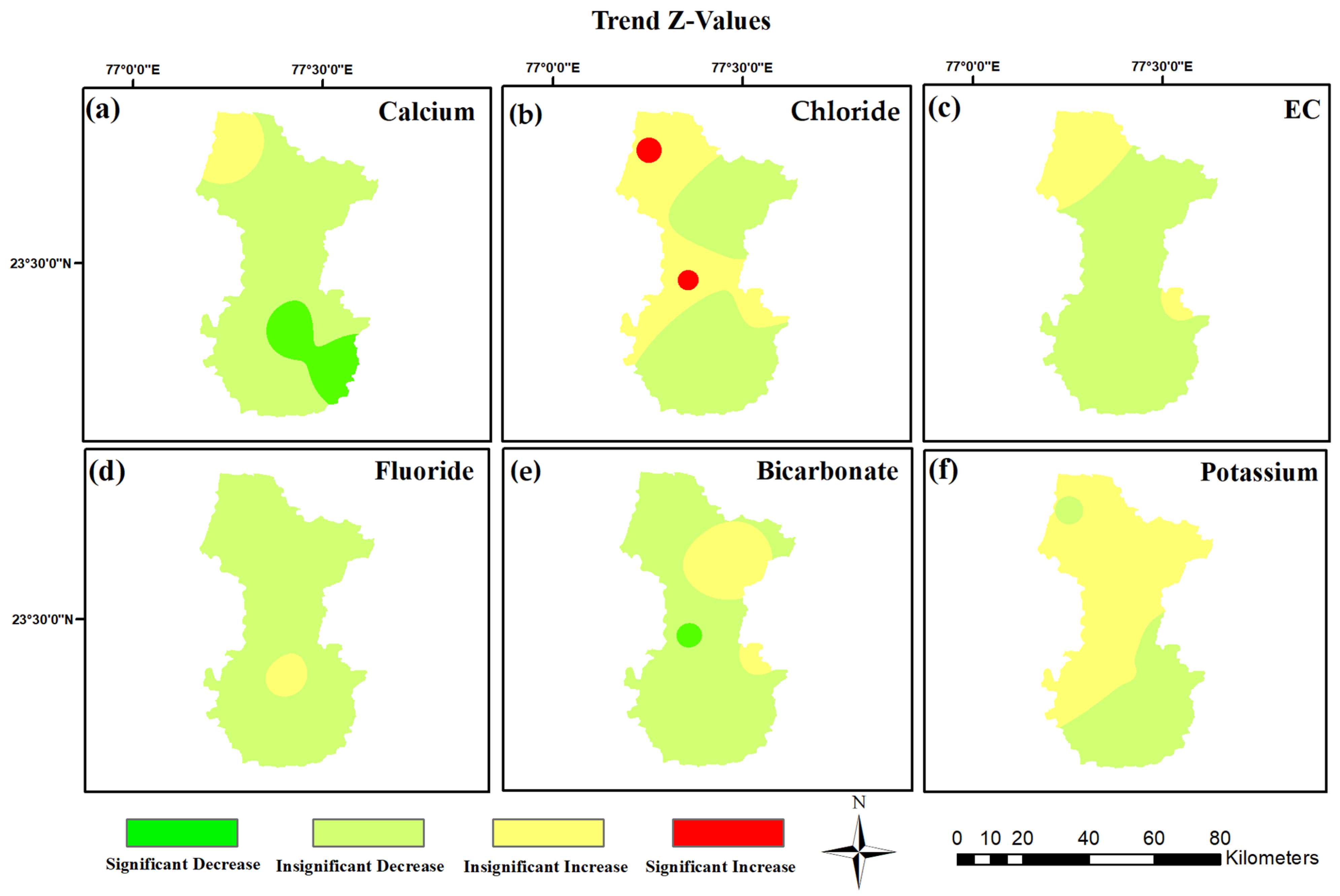
Sen’s slope, ‘S’, detects the numerical levels of a trend, while statistics, ‘Z’, determines whether there is an upward or downward movement in the trend of data in a time series. A positive value for Z represents an increase in the concentration of a component over time, whereas a negative value for Z indicates a decrease. To determine the confidence level percentage, one can subtract the probability (p) from 1, resulting in Confidence = (1 − p) percent. For instance, 0.1 represents a 90 percent confidence level, 0.05 represents a 95 percent confidence level, and 0.01 represents a 99 percent confidence level. The Mann-Kendall (MK) and Modified Mann-Kendall (MMK) trend tests used in this study have a 95% confidence level. The S-value (shown in Figure 4) and Z-value (shown in Figure 5 and Figure 6) were estimated. The increasing and decreasing trend (Z-value) of various parameters has been shown using Arc-GIS by inverse distance weighted (IDW) interpolation of Z-values over the study area [32].

For the study on MK trends and Sen’s Slope, the collected groundwater data samples from 22 consecutive years, from 2000 to 2021, have been analyzed for 12 chemical parameters. The magnitudes of Ca²⁺, Mg²⁺, K⁺, Na⁺, Cl⁻, SO₄²⁻, NO₃⁻, bicarbonate (HCO₃⁻), total hardness (TH), pH, electrical conductivity, and fluoride were considered (Figure 4). On applying MK and MMK tests, most parameters showed a mixture of positive (H-value equals 1) and negative (H-value equals 0) trends. All trend results were the same for all parameters in the MK and MMK tests except for pH and total hardness. For pH, the MK test did not give any positive results for any station in Bhopal. In contrast, the MMK test showed a positive outcome for two stations, i.e., Berasia and Islamnagar. Additionally, MMK gave a positive result for total hardness for Nagirabad (

Table 3. Results of trend analysis of various groundwater hydro-chemical parameters in Bhopal.

Parameter	Location	Latitude	Longitude	Mann Kendall			Modified Mann Kendall
				p-Value	Z-Value	Sen’s Slope	p-Value	Z-Value	Sen’s Slope
Ca2+	Balampurghati	23.397	77.542	0.414	−0.818	−0.400	0.414	−0.818	−0.400
	Berasia	23.623	77.431	0.091	−1.692	−2.211	0.091	−1.692	−2.211
	Bilkhiria	23.256	77.580	0.015	−2.425	−2.000	0.015	−2.425	−2.000
	Islamnagar	23.357	77.416	0.008	−2.651	−4.000	0.001	−3.356	−4.000
	Gunga	23.450	77.360	0.693	−0.395	−0.476	0.693	−0.395	−0.476
	Nagirabad	23.794	77.256	0.592	0.536	0.444	0.592	0.536	0.444
Cl−	Balampurghati	23.397	77.542	0.414	0.818	1.246	0.291	1.057	1.246
	Berasia	23.623	77.431	0.063	−1.861	−2.333	0.063	−1.861	−2.333
	Bilkhiria	23.256	77.580	0.554	−0.592	−1.000	0.554	−0.592	−1.000
	Islamnagar	23.357	77.416	0.071	−1.805	−1.553	0.071	−1.805	−1.553
	Gunga	23.450	77.360	0.021	2.312	3.538	0.021	2.312	3.538
	Nagirabad	23.794	77.256	0.040	2.058	5.976	0.040	2.058	5.976
EC	Balampurghati	23.397	77.542	0.573	0.564	6.125	0.573	0.564	6.125
	Berasia	23.623	77.431	0.215	−1.241	−11.714	0.215	−1.241	−11.714
	Bilkhiria	23.256	77.580	0.430	−0.790	−12.821	0.430	−0.790	−12.821
	Islamnagar	23.357	77.416	0.091	−1.692	−13.250	0.091	−1.692	−13.250
	Gunga	23.450	77.360	0.735	−0.338	−3.000	0.735	−0.338	−3.000
	Nagirabad	23.794	77.256	0.195	1.297	15.889	0.195	1.297	15.889
F−	Balampurghati	23.397	77.542	0.011	−2.538	−0.016	0.011	−2.538	−0.016
	Berasia	23.623	77.431	0.955	−0.056	−0.001	0.955	−0.056	−0.001
	Bilkhiria	23.256	77.580	0.076	−1.776	−0.013	0.076	−1.776	−0.013
	Islamnagar	23.357	77.416	0.367	0.902	0.006	0.367	0.902	0.006
	Gunga	23.450	77.360	0.338	−0.959	−0.007	0.338	−0.959	−0.007
	Nagirabad	23.794	77.256	0.040	−2.058	−0.029	0.040	−2.058	−0.029
HCO3−	Balampurghati	23.397	77.542	0.592	0.536	0.857	0.375	0.886	0.857
	Berasia	23.623	77.431	0.414	0.818	2.863	0.414	0.818	2.863
	Bilkhiria	23.256	77.580	0.338	−0.959	−3.143	0.338	−0.959	−3.143
	Islamnagar	23.357	77.416	0.535	−0.620	−2.091	0.535	−0.620	−2.091
	Gunga	23.450	77.360	0.021	−2.312	−7.714	0.021	−2.312	−7.714
	Nagirabad	23.794	77.256	0.517	−0.649	−1.680	0.192	−1.304	−1.680
K+	Balampurghati	23.397	77.542	0.114	−1.579	−0.083	0.114	−1.579	−0.083
	Berasia	23.623	77.431	0.195	1.297	0.031	0.321	0.992	0.031
	Bilkhiria	23.256	77.580	0.414	−0.818	−0.067	0.414	−0.818	−0.067
	Islamnagar	23.357	77.416	0.978	0.028	0.060	0.978	0.028	0.060
	Gunga	23.450	77.360	0.367	0.902	0.030	0.367	0.902	0.030
	Nagirabad	23.794	77.256	0.978	−0.028	0.000	0.978	−0.028	0.000
Mg2+	Balampurghati	23.397	77.542	0.844	−0.197	−0.055	0.844	−0.197	−0.055
	Berasia	23.623	77.431	0.225	1.213	0.552	0.225	1.213	0.552
	Bilkhiria	23.256	77.580	1.000	0.000	0.000	1.000	0.000	0.000
	Islamnagar	23.357	77.416	0.978	−0.028	−0.005	0.962	−0.047	−0.005
	Gunga	23.450	77.360	1.000	0.000	0.000	1.000	0.000	0.000
	Nagirabad	23.794	77.256	0.592	0.536	0.774	0.530	0.628	0.774
Na+	Balampurghati	23.397	77.542	0.030	2.171	1.060	0.030	2.171	1.060
	Berasia	23.623	77.431	0.888	0.141	0.125	0.888	0.141	0.125
	Bilkhiria	23.256	77.580	0.978	−0.028	−0.164	0.947	−0.066	−0.164
	Islamnagar	23.357	77.416	0.271	1.100	0.757	0.271	1.100	0.757
	Gunga	23.450	77.360	0.778	−0.282	−0.250	0.778	−0.282	−0.250
	Nagirabad	23.794	77.256	0.778	0.282	0.516	0.778	0.282	0.516
NO3−	Balampurghati	23.397	77.542	0.735	0.338	0.182	0.735	0.338	0.182
	Berasia	23.623	77.431	0.011	−2.538	−2.725	0.011	−2.538	−2.725
	Bilkhiria	23.256	77.580	0.844	0.197	0.143	0.844	0.197	0.143
	Islamnagar	23.357	77.416	0.248	−1.156	−1.154	0.248	−1.156	−1.154
	Gunga	23.450	77.360	0.195	−1.297	−1.100	0.195	−1.297	−1.100
	Nagirabad	23.794	77.256	1.000	0.000	0.000	1.000	0.000	0.000
pH	Balampurghati	23.397	77.542	0.414	−0.818	−0.008	0.093	−1.678	−0.008
	Berasia	23.623	77.431	0.128	1.523	0.011	0.001	3.195	0.011
	Bilkhiria	23.256	77.580	0.978	0.028	0.000	0.978	0.028	0.000
	Islamnagar	23.357	77.416	0.248	−1.156	−0.008	0.017	−2.376	−0.008
	Gunga	23.450	77.360	0.822	−0.226	−0.001	0.822	−0.226	−0.001
	Nagirabad	23.794	77.256	0.672	0.423	0.006	0.635	0.475	0.006
SO42−	Balampurghati	23.397	77.542	0.143	1.466	0.748	0.143	1.466	0.748
	Berasia	23.623	77.431	0.259	−1.128	−0.613	0.259	−1.128	−0.613
	Bilkhiria	23.256	77.580	0.735	−0.338	−0.200	0.735	−0.338	−0.200
	Islamnagar	23.357	77.416	0.037	−2.087	−1.435	0.037	−2.087	−1.435
	Gunga	23.450	77.360	0.888	0.141	0.169	0.888	0.141	0.169
	Nagirabad	23.794	77.256	0.735	−0.338	−0.333	0.735	−0.338	−0.333
TH	Balampurghati	23.397	77.542	0.672	−0.423	−1.417	0.672	−0.423	−1.417
	Berasia	23.623	77.431	0.324	−0.987	−3.200	0.324	−0.987	−3.200
	Bilkhiria	23.256	77.580	0.135	−1.494	−7.313	0.135	−1.494	−7.313
	Islamnagar	23.357	77.416	0.032	−2.143	−8.374	0.032	−2.143	−8.374
	Gunga	23.450	77.360	1.000	0.000	0.000	1.000	0.000	0.000
	Nagirabad	23.794	77.256	0.430	0.790	5.145	0.023	2.272	5.145

).

The Sen’s slope value for MK and MMK was the same for all 12 parameters, whereas the p-value and the Z-Value were marginally different for all parameters in both tests (Table 3). An insignificant trend in MK and MMK trend tests for EC, K^+, and Mg²⁺ was found over all stations of Bhopal (Figure 5 and Figure 6); in the case of calcium, two stations gave positive results for the MK and MMK test in which Bilkhiria gave a decreasing trend, and Islamnagar showed an increasing trend with Sen’s slopes of −8.374 mg/L/year and 5.145 mg/L/year, respectively. Only a single station gave a positive trend for sulfate, nitrate, sodium, and bicarbonate. In Balampurghati, sodium showed an increasing trend in both tests with a Sen’s slope of 1.06 mg/L/year. A decreasing trend was found in Islamnagar for sulfate, Berasia for nitrate, and Gunga for bicarbonate with a Sen’s slope of −1.435 mg/L/year, −2.725 mg/L/year, and −7.714 mg/L/year for all three stations, respectively. For fluoride, a decreasing trend was seen for Balampurghati and Nagirabad, with a Sen’s slope value of −0.016 mg/L/year and −0.029 mg/L/year, respectively. Whereas, for chloride, a positive trend was seen for Gunga and Nagirabad, with Sen’s slopes of 3.538 mg/L/year and 5.976 mg/L/year, respectively. The MK test revealed a decreasing trend in total hardness in Islamnagar with a Sen’s slope of −8.374 mg/L/year. In addition, the MMK test found an increasing trend in total hardness in Nagirabad with a Sen’s slope of 5.145 mg/L/year. Only the MMK test found positive trends for pH at Bilkhiria and Islamnagar, with Sen’s slopes of 0.011 mg/L/year and −0.008 mg/L/year, respectively.

4. Conclusions

Assessment of groundwater levels from year 2000 to 2020 shows that increased surface and groundwater conservation activities have improved the groundwater table in Bhopal. The study also analyzed chemical properties and revealed that the groundwater in the area was mainly classified as hard to very hard, with levels exceeding the permissible limits at Nagirabad. Furthermore, two wells in the district had nitrate content that surpassed the acceptable limit. Nitrate levels were high at two locations in Islamabad and Sarvar, the regular consumption of which can lead to blue-baby disease. Islamnagar and Balampurghati are the sites within the district where values exceeded the acceptable limits for EC and pH, respectively.

This study examined water quality trends between 2000–2021 using the Mann-Kendall, Modified Mann-Kendall, and Sen’s Slope methods with a 95% confidence level. The results revealed mixed trends, including both positive and negative trends. While the MK and MMK trend tests for EC, K⁺, and Mg²⁺ showed no trends, an increasing trend was observed in Na⁺ and Cl⁻. Conversely, parameters such as SO₄²⁻, Ca²⁺, HCO₃⁻, NO₃⁻, and F⁻ showed a negative trend, with mixed trends only observed in pH. It is evident from the analysis that two of the wells have already crossed the acceptable limits for domestic purposes (as per Indian Standards). If present conditions persist, chloride levels will also cross the desired limits, and groundwater’s hardness level will worsen in Gunga and Nagirabad, respectively. This study emphasizes that the MMK trend test gives efficient results in hydrogeological settings of the Deccan Trap compared to the MK trend test; for the Vindhyan supergroup, both MK and MMK trend tests can be used. Further research over a consistent time period is necessary to establish any spatial patterns. Regular monitoring and evaluation of groundwater quality and quantity is essential for taking appropriate measures to monitor contamination to ensure the availability of safe water.

References

- Li, W.; Wu, J.; Zhou, C.; Nsabimana, A. Groundwater Pollution Source Identification and Apportionment Using PMF and PCA-APCS-MLR Receptor Models in Tongchuan City, China. Arch. Environ. Contam. Toxicol. 2021, 81, 397–413. [Google Scholar] [CrossRef] [PubMed]
- Jeon, C.; Raza, M.; Lee, J.Y.; Kim, H.; Kim, C.S.; Kim, B.; Kim, J.W.; Kim, R.H.; Lee, S.W. Countrywide Groundwater Quality Trend and Suitability for Use in Key Sectors of Korea. Water 2020, 12, 1193. [Google Scholar] [CrossRef]
- Duggal, V.; Rani, A. Carcinogenic and Non-Carcinogenic Risk Assessment of Metals in Groundwater via Ingestion and Dermal Absorption Pathways for Children and Adults in Malwa Region of Punjab. J. Geol. Soc. India 2018, 92, 187–194. [Google Scholar] [CrossRef]
- Duggal, V.; Rani, A.; Mehra, R.; Balaram, V. Risk Assessment of Metals from Groundwater in Northeast Rajasthan. J. Geol. Soc. India 2017, 90, 77–84. [Google Scholar] [CrossRef]
- Karunanidhi, D.; Aravinthasamy, P.; Deepali, M.; Subramani, T.; Shankar, K. Groundwater Pollution and Human Health Risks in an Industrialized Region of Southern India: Impacts of the COVID-19 Lockdown and the Monsoon Seasonal Cycles. Arch. Environ. Contam. Toxicol. 2021, 80, 259–276. [Google Scholar] [CrossRef]
- Wahlin, K.; Grimvall, A. Roadmap for Assessing Regional Trends in Groundwater Quality. Environ. Monit. Assess. 2010, 165, 217–231. [Google Scholar] [CrossRef]
- Dhayachandhran, K.S.; Jothilakshmi, M. Quality Assessment of Ground Water along the Banks of Adyar River Using GIS. Mater. Today Proc. 2020, 45, 6234–6241. [Google Scholar] [CrossRef]
- Frollini, E.; Preziosi, E.; Calace, N.; Guerra, M.; Guyennon, N.; Marcaccio, M.; Menichetti, S.; Romano, E.; Ghergo, S. Groundwater quality trend and trend reversal assessment in the European Water Framework Directive context: An example with nitrates in Italy. Environ. Sci. Pollut. Res. 2021, 28, 22092–22104. [Google Scholar] [CrossRef]
- Mustapha, A. Detecting Surface Water Quality Trends Using Mann-Kendall Tests and Sen’s Slope Estimates. Int. J. Agric. Innov. Res. 2013, 1, 108–114. [Google Scholar]
- Batlle Aguilar, J.; Orban, P.; Dassargues, A.; Brouyère, S. Identification of Groundwater Quality Trends in a Chalk Aquifer Threatened by Intensive Agriculture in Belgium. Hydrogeol. J. 2007, 15, 1615–1627. [Google Scholar] [CrossRef]
- Amirataee, B.; Zeinalzadeh, K. Trends Analysis of Quantitative and Qualitative Changes in Groundwater with Considering the Autocorrelation Coefficients in West of Lake Urmia, Iran. Environ. Earth Sci. 2016, 75, 371. [Google Scholar] [CrossRef]
- Broers, H.P.; Van Der Grift, B. Regional Monitoring of Temporal Changes in Groundwater Quality. J. Hydrol. 2004, 296, 192–220. [Google Scholar] [CrossRef]
- Swain, S.; Sahoo, S.; Taloor, A.K.; Mishra, S.K.; Pandey, A. Exploring Recent Groundwater Level Changes Using Innovative Trend Analysis (ITA) Technique over Three Districts of Jharkhand, India. Groundw. Sustain. Dev. 2022, 18, 100783. [Google Scholar] [CrossRef]
- Central Ground Water Board. Bhopal District Profile; Ministry of Water Resources: Faridabad, India, 2013.
- Central Ground Water Board. Ground Water Year Book—Madhya Pradesh; Central Ground Water Board: Faridabad, India, 2018.
- Central Ground Water Board. Dynamic Groundwater Resources of Madhya Pradesh; Central Ground Water Board: Faridabad, India, 2022.
- Patil, S. Situation Analysis of Groundwater in Madhya Pradesh; Central Ground Water Board: Faridabad, India, 2019.
- Mishra, S.; Suresh, S.; Chauhan, M.S.; Subbaramaiah, V.; Gosu, V. Recent Progress in Carbonaceous Materials for the Nitrate Adsorption. J. Hazardous Toxic Radioact. Waste 2022, 26, 04022013. [Google Scholar] [CrossRef]
- Raj, V.; Chauhan, M.S.; Pal, S.L. Potential of Sugarcane Bagasse in Remediation of Heavy Metals: A Review. Chemosphere 2022, 307, 135825. [Google Scholar] [CrossRef]
- Rangabhashiyam, S.; Lins, P.V.d.S.; Oliveira, L.M.T.d.M.; Sepulveda, P.; Ighalo, J.O.; Rajapaksha, A.U.; Meili, L. Sewage Sludge-Derived Biochar for the Adsorptive Removal of Wastewater Pollutants: A Critical Review. Environ. Pollut. 2022, 293, 118581. [Google Scholar] [CrossRef]
- Central Ground Water Board. Ground Water Year Book Madhya Pradesh (2021–2022); Central Ground Water Board: Faridabad, India, 2021.
- IS 10500; BIS Indian Standard Drinking Water Specification (Second Revision). Bureau of Indian Standards: Delhi, India, 2012.
- WHO. Water Quality for Drinking: WHO Guidelines; WHO: Geneva, Switzerland, 2012. [Google Scholar]
- Roy, S.; Taloor, A.K.; Bhattacharya, P. A Geospatial Approach for Understanding the Spatio-Temporal Variability and Projection of Future Trend in Groundwater Availability in the Tawi Basin, Jammu, India. Groundw. Sustain. Dev. 2023, 21, 100912. [Google Scholar] [CrossRef]
- Daneshvar Vousoughi, F.; Dinpashoh, Y.; Aalami, M.T.; Jhajharia, D. Trend Analysis of Groundwater Using Non-Parametric Methods (Case Study: Ardabil Plain). Stoch. Environ. Res. Risk Assess. 2013, 27, 547–559. [Google Scholar] [CrossRef]
- Patakamuri, S.K.; Muthiah, K.; Sridhar, V. Long-Term Homogeneity, Trend, and Change-Point Analysis of Rainfall in the Arid District of Ananthapuramu, Andhra Pradesh State, India. Water 2020, 12, 211. [Google Scholar] [CrossRef]
- Duggal, V.; Sharma, S. Fluoride Contamination in Drinking Water and Associated Health Risk Assessment in the Malwa Belt of Punjab, India. Environ. Adv. 2022, 8, 100242. [Google Scholar] [CrossRef]
- Balderacchi, M.; Benoit, P.; Cambier, P.; Eklo, O.M.; Gargini, A.; Gemitzi, A.; Gurel, M.; Kløve, B.; Nakic, Z.; Predaa, E.; et al. Groundwater Pollution and Quality Monitoring Approaches at the European Level. Crit. Rev. Environ. Sci. Technol. 2013, 43, 323–408. [Google Scholar] [CrossRef]
- Huan, H.; Li, X.; Zhou, J.; Liu, W.; Li, J.; Liu, B.; Xi, B.; Jiang, Y. Groundwater Pollution Early Warning Based on QTR Model for Regional Risk Management: A Case Study in Luoyang City, China. Environ. Pollut. 2020, 259, 113900. [Google Scholar] [CrossRef] [PubMed]
- Sarath Prasanth, S.V.; Magesh, N.S.; Jitheshlal, K.V.; Chandrasekar, N.; Gangadhar, K. Evaluation of Groundwater Quality and Its Suitability for Drinking and Agricultural Use in the Coastal Stretch of Alappuzha District, Kerala, India. Appl. Water Sci. 2012, 2, 165–175. [Google Scholar] [CrossRef]
- El Alfy, M.; Lashin, A.; Abdalla, F.; Al-Bassam, A. Assessing the Hydrogeochemical Processes Affecting Groundwater Pollution in Arid Areas Using an Integration of Geochemical Equilibrium and Multivariate Statistical Techniques. Environ. Pollut. 2017, 229, 760–770. [Google Scholar] [CrossRef]
- Vishwakarma, A.; Choudhary, M.K.; Chauhan, M.S. Applicability of Spi and Rdi for Forthcoming Drought Events: A Non-Parametric Trend and One Way Anova Approach. J. Water Clim. Chang. 2020, 11, 18–28. [Google Scholar] [CrossRef]