Public Transport Modeling for Commuting in Cities with Different Development Levels Using Extended Theory of Planned Behavior

Abstract

Reducing the use of private vehicles and promoting public transportation (PT) have always been the primary policy objectives of transport authorities. This study aims to model the factors affecting intentions and behaviors of employees to use PT for their commutes by creating an extended theory of planned behavior (ETPB). The ETPB model’s applicability was evaluated using the Partial Least Squares Structural Equation Model (PLS-SEM) technique on a total of 2048 employees in three distinct cities. Then, the Multigroup analysis (MGA) method was used to compare various cities, and demographic variables such as age, education, gender, household income, and walking time to nearest PT stop. The analysis revealed that attitude, perceived norm, and personal agency have a statistically positive influence on employees’ intention to use PT. Moreover, behavioral capability, intention, and habit have a positive effect on PT use, whereas environmental constraints have a negative effect. The results of the MGA analysis revealed significant differences between regions, particularly in terms of environmental factors, intention, and habit. Similarly, the article describes disparities that have emerged according to other demographic variables. The findings imply that interventions by decision makers have the potential to alter the mode of transportation chosen for commuting.

1. Introduction

As a result of the employment opportunities offered by immigration, traffic congestion occurs in cities that have begun to receive a greater number of immigrants, causing economic and environmental issues [1]. The aforementioned circumstances require the development of sustainable transportation plans by professionals in the field of transportation planning. Public transportation (PT) systems generally exhibit a reduced emission rate per passenger in comparison to private vehicles, thereby yielding environmental advantages. The implementation of clean energy sources and the optimization of routes in PT systems can effectively mitigate greenhouse gas emissions, air pollution, and energy consumption, thereby making a significant contribution towards the creation of a more environmentally sustainable ecosystem [2]. The reduction in traffic congestion can be attributed to the increasing preference for PT, which leads to a decrease in the presence of private vehicles on the road. Not only does this practice result in time efficiency for individuals who commute, but it also contributes to fuel conservation and enhanced air quality [3]. The promotion of compact urban growth is frequently facilitated by PT, hence enhancing land use efficiency. By promoting increased population density in proximity to transportation centers, it optimizes the utilization of land, mitigates urban sprawl, and safeguards natural regions against superfluous development [4].

The mechanism for selecting a mode of transportation is shaped by the intricate structure of human behavior and by one’s way of life [5]. Therefore, policymakers and transport administrators must comprehend passenger behavior and identify the factors that will encourage them to utilize public transportation. In order to accomplish this, a comprehensive study is required to ascertain the factors that influence the mode of transportation chosen by commuters [6].

Due to the relevance of home-to-work commutes during congested peak periods and to transit markets, home-based work (HBW) trips are of particular significance [7]. Currently, both traditional four-stage models and activity-based models are employed in public transportation planning. Traditional and advanced travel models are typically based on a core set of probabilistic choice models. Household surveys, socioeconomic characteristics, and spatial determinants are used to develop these models [8]. To ensure the long-term viability of PT and to enable transport policymakers to implement interventions that encourage the use of PT, it is necessary to also consider the psychosocial determinants of the area’s residents [9].

In this study, developed (Antalya), developing (Erzurum), and underdeveloped (Igdir) cities in Turkey were surveyed for their psychosocial perspectives on the use of public transportation for HBW trips. Transportation and infrastructure data were obtained from the Turkish Statistical Institute (TUIK) [10]. For three cities, the Planned Behavior Theory (TPB) model was tested with the addition of instrumental attitude, descriptive norm, self-efficacy, knowledge and skills, habit, and environmental constraints. The primary contribution of this article is to fill a gap in the literature by analyzing the factors influencing home-to-work commuters’ choice of public transportation mode in cities with three distinct levels of development and by comparing various demographic variables. This article concentrates on the analysis of psychosocial determinants that influence the choice of mode of transportation using the extended version of the TPB model and the Partial Least Squares Structural Equation Model (PLS-SEM) technique. Without a greater understanding of the psychosocial perspectives of residents who use public transportation towards the current system, the current system’s ability to direct users to public transportation will not be efficient [11]. In light of this, understanding the psychosocial determinants of user behavior will aid policymakers in their efforts to promote the use of PT for sustainability.

2. Materials and Methods

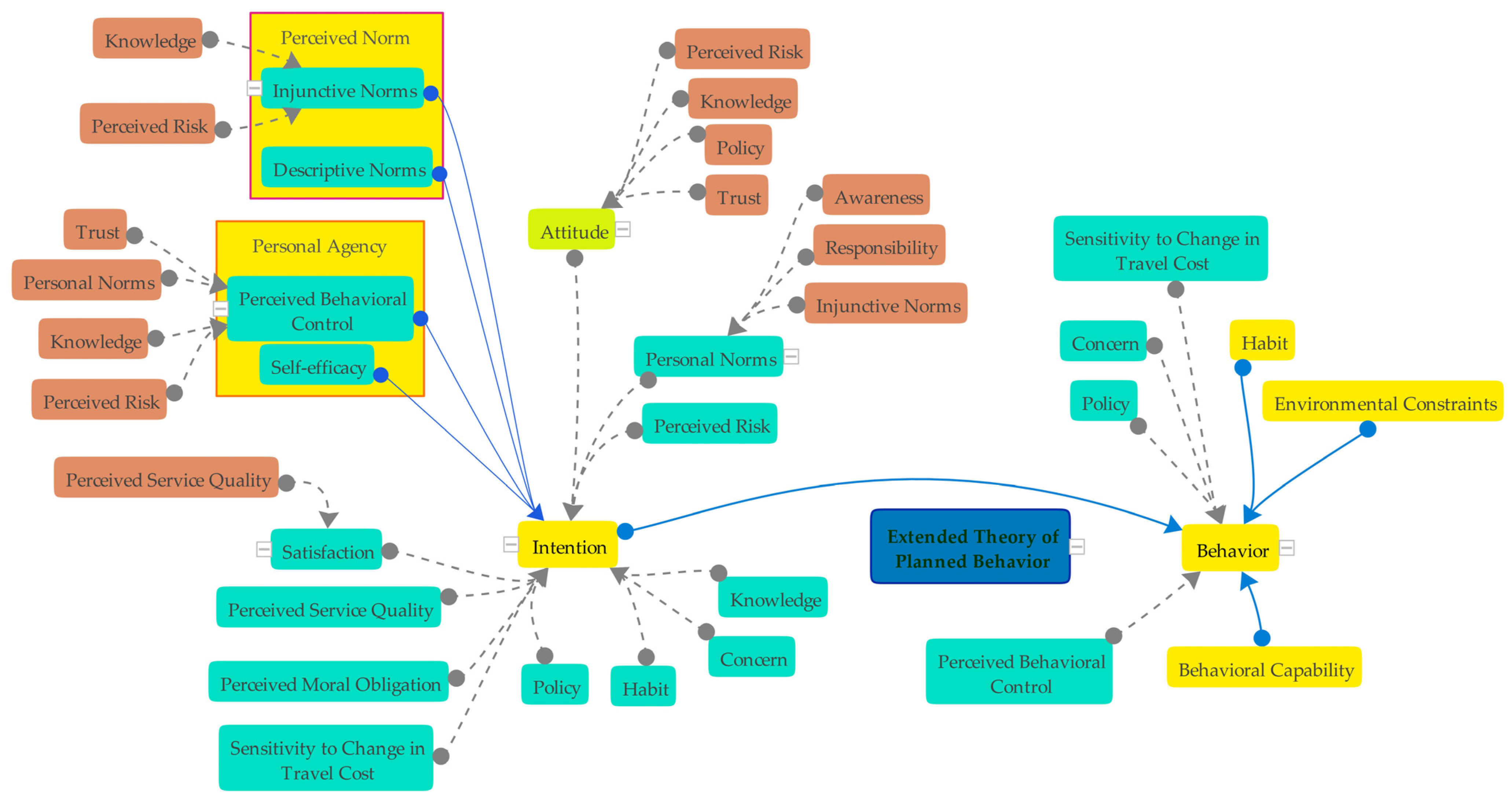
2.1. Extended Theory of Planned Behavior (ETPB)

Ajzen [12] devised the paradigm of the theory of planned behavior (TPB) to comprehend rather than predict human behavior. Decision-making is an extremely difficult process for individuals. Principally influencing behavior is the intent to partake in the behavior. It is unlikely that the individual will engage in the behavior unless they intend to. However, when there is a desire to act in a particular manner, i.e., intention, there are three crucial factors at play. First, attitudes (ATT) are a person’s comprehensive evaluation of an intention, taking both instrumental and experiential factors into account [13]. The second factor is the subjective norm (SN), or how probable it is that others will perceive the behavior. The third factor is perceived behavior control (PBC), or the degree to which a subject believes they have control over a particular activity [12].

In addition to the above-mentioned three factors, there are additional factors that influence intention, such as descriptive norm (DN), which can be defined as an essential component of normative influence [13,14,15,16].

Besides intention, four additional factors have a direct influence on behavior [17]. Three of these factors are crucial for determining whether behavioral intentions can lead to behavioral performance. The individual must possess the requisite knowledge and skills to execute the act. Additionally, there should be few or no environmental restrictions that make displaying the behavior difficult or impossible [13]. Third, for a person to remember to engage in an activity, it must be prominent in their mind [18]. Last but not least, repetition of an action may cause it to become habitual, reducing the importance for these individuals to base their behavior on their intentions [13,19,20].

2.2. ETPB Models in Travel-Related Activities

TPB has been extensively utilized in numerous transport-related behavior prediction models [21]. Bamberg et al. [22] introduced prepaid bus tickets as an innovation to encourage college students to take the bus more frequently. According to the theory, the intervention was shown to have the desired effect on intentions and behavior by influencing attitudes toward bus use, subjective norms, and PBC. Similarly, after the implementation of a universal bus pass among college students at a Canadian institution, Heath and Gifford [23] discovered a significant positive association between self-reported bus usage and the intention to use a bus, which is positively associated with attitudes regarding bus use, the subjective norm, and the PBC.

As the importance of sustainability grows, TPB models have been expanded and enhanced to maintain sustainable transportation options [24,25,26,27]. Liu et al. [28] proposed an integrated model based on the norm activation model (NAM) and the TPB to predict people’s intentions to reduce their vehicle use in China. Chen et al. [29] developed a mixed pro-environment travel behavior (PET) model by extending the TPB by incorporating the effects of public transport quality, commuter satisfaction, and habit. Hu et al. [30] constructed a modified theory of planned behavior (MTPB) model framework by adding two additional factors, namely, environmental concern and moral obligation, in order to comprehend young people’s intention to engage in low-carbon travel. In addition to the TPB factors, moral obligation and environmental concern were found to correlate positively with intention. Ibrahim et al. [31] modified the TPB using “trust” to determine if it can account for consumers’ intentions to use park-and-ride (P&R) bus services in Putrajaya, Malaysia. Zhang et al. [32] examined the sensitivity of commuters to changes in travel costs. A traveler’s sensitivity to changes in travel amenities has the greatest impact on their intentions and actual mode-choice behavior, according to the findings of the analysis.

The majority of the aforementioned studies have examined people’s preferences for private or commuter travel within a specific geographic region. However, geographic disparity research is an uncommon exception. Lo et al. [33] investigated the effects of organizational sector and geographic location on the Extended Theory of Planned Behavior (ETPB) model of commuting travel mode selection. Many commute-related perceptions varied between organizational domains and geographic locations, according to a study. The significance of psychosocial drivers in the ETPB model was typically consistent across industries and geographies, with the exception of the influence of injunctive norms, which varied by region. Li et al. [34] incorporated low-carbon transportation policy, psychological factors, social norms, and habits to examine whether or not there are regional and generational differences in the intention to employ low-carbon transport options. The findings revealed geographical and generational variation in the effect on the intention to engage in low-emission travel behavior. Although regional and sociocultural differences have been studied, insufficient literature exists about the ETPB model, in which environmental restrictions can also be measured in cities such as Turkey, where the transportation infrastructure varies substantially. Figure 1 illustrates various use and application variations of the ETPB paradigm as documented in the literature. The parameters highlighted in yellow within the graphic represent the components of the ETPB model as utilized in this particular study.

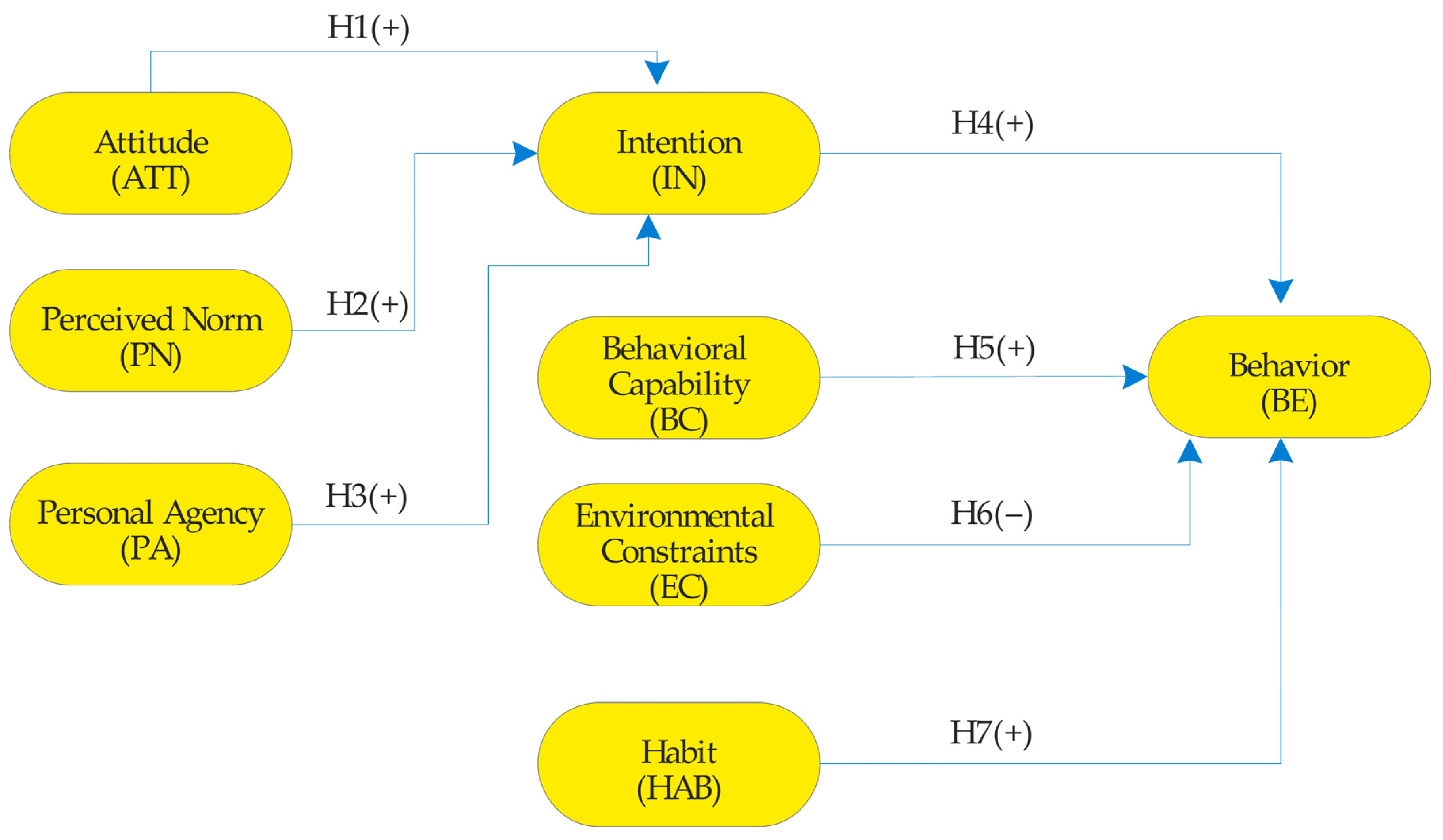
2.3. Research Hypotheses

The TPB model, which has been deemed effective at predicting and describing human behavior, has been effectively tested by incorporating additional variables. The purpose of this study is to predict intention and behavior by adding some new parameters to the existing ETPB model. The ETPB model devised to select PT as the mode of transport for HBW trips is depicted in Figure 2.

2.3.1. Attitude (ATT)

The TPB asserts that attitude is the most influential factor on behavioral intention. An individual’s demeanor reflects how they feel about the potential outcomes of an endeavor. Specifically, this attitude comprises a person’s significant beliefs about the outcomes of a behavior as well as his or her evaluation of the outcomes as positive or negative. The individual’s overall attitude toward the activity is then determined by averaging their positive and negative perceptions [12]. Therefore, attitude can be viewed as a crucial factor in describing and predicting human behavior. In this study, commuters’ attitudes and propensities toward PT are inferred from their behavior toward this practice. According to the empirical data, it is plausible to assume that travelers are more likely to have a positive attitude toward PT if they believe it will assist them in achieving their own objectives. Based on the aforementioned points of view, this investigation proposes the following hypothesis:

Hypothesis 1 (H1):

The behavioral attitude of commuters is positively associated with their intention to utilize PT.

2.3.2. Perceived Norm (PN)

The perceived norm is the social pressure one feels to perform or refrain from performing a particular action. According to the proposed TPB model, the subjective norm is the perception of whether or not the majority of individuals concur with the conduct. It depends on whether the individual’s colleagues and significant others believe he or she should engage in the behavior. In addition to subjective norms, a person may also perceive normative pressure if they perceive that influential individuals are engaging in or refraining from problematic behavior. Both types of normative pressure have the capacity to influence behavior. These two types of norms are known, respectively, as injunctive and descriptive [12,13]. According to the studies, descriptive and subjective norms substantially predicted the use of vehicle and bus modes [25,35,36]. Consequently, the perceived norm is regarded as a crucial ambiguity for monitoring and predicting behavioral intention. On this basis, the following hypothesis is advanced in this study:

Hypothesis 2 (H2):

A positive correlation exists between the perceived norm of commuters and their intention to use PT.

2.3.3. Personal Agency (PA)

Due to the large number of elements and the lack of an exhaustive definition of PBC, researchers decided to investigate the construct’s dimensionality [37]. Consequently, support for two fundamental components became apparent, prompting Ajzen [38] to redefine PBC as an overall construct with two distinct but interconnected subcomponents: “controllability” and “self-efficacy”. The personal agency (PA) factor was introduced by adding self-efficacy to the concept of perceived control [39]. Self-efficacy is a person’s confidence in their ability to carry out their behavior in the face of various obstacles or problems. Montano et al. [40] demonstrate the value of incorporating both measures, despite the fact that few studies have analyzed the similarities and differences between these two notions [38,41]. According to studies, self-efficacy, like perceived behavioral control, has a positive effect on the intention to take PT [42,43,44,45]. In this study, it is hypothesized that personal agency may have a direct effect on the prediction of intentions. On this basis, the following hypothesis is advanced below:

Hypothesis 3 (H3):

There is a positive correlation between commuters’ personal agency and their intention to utilize PT.

2.3.4. Intention (IN)

Behavioral intentions are indicators of a person’s readiness to engage in a particular behavior. A person’s estimation of the likelihood or perceived probability of carrying out a specific behavior is the defining characteristic of an intention. Researchers anticipate that the greater this subjective possibility, the greater the likelihood that the behavior will occur [12,13]. The ETPB’s behavioral intention can be expressed in its basic form using the following mathematical formula:

IN = _wATTATT + _wPNPN + _wPAPA

(1)

where w is an empirically derived weight or coefficient. In studies examining the behavior of individuals utilizing PT, the positive effect of intention on behavior has been demonstrated. Taking into account this direct impact, the following hypothesis has been proposed:

Hypothesis 4 (H4):

There is a positive correlation between the intentions of commuters and their actual use of PT.

2.3.5. Behavioral Capability (BC)

In numerous studies utilizing the TPB model, it has been seen that knowledge and ability are measured independently of one another [46,47,48,49]. Despite the fact that knowledge has a substantial cognitive influence on behavior, it is typically insufficient to generate behavior change on its own. Numerous behaviors necessitate the acquisition of a variety of specialized skills in order to be executed correctly. Knowledge and abilities produce behavioral capability (BC) [50]. Using the behavioral ability factor, a number of studies on the behavior of using sustainable transport systems have been well documented in the literature [26,27,51]. Despite the lack of studies employing both knowledge and skills to forecast travel choice behavior, behavioral research in the health sciences predicts that BC will be influential in public transport use behavior:

Hypothesis 5 (H5):

The relationship between commuters’ behavioral capability and their PT use behavior is positive.

2.3.6. Environmental Constraints (EC)

Fishbein and Ajzen [13] introduced an expanded variant of TPB that included environmental constraints (EC). In the context of the TPB, EC refers to external conditions that may limit an individual’s capacity to engage in a specific behavior. These reasons may include physical, social, and economic obstacles that hinder or make it difficult for an individual to carry out their goals [13]. Numerous studies have investigated the effect of EC on behavior in the context of the TPB [52]. In addition, the Integrated Behavior Model (IBM) derived from the TPB has demonstrated that EC can directly influence behavior [53]. EC are an essential component of the TPB because they may influence an individual’s ability to perform a behavior and should be taken into account when designing interventions to promote behavior change. In this study, it is hypothesized that EC may have a direct negative influence on PT use:

Hypothesis 6 (H6):

There is a negative correlation between commuters’ environmental consciousness and their PT use behavior.

2.3.7. Habit (HAB)

Habits are automatic, learned behaviors performed without conscious thought or effort; they can either strengthen or diminish intentions to engage in a behavior [54]. An increasing number of studies have focused on the significance of patterns in TPB and their influence on behavior [24,25,54]. In general, these studies indicate that habits are important factors to be considered in the TPB, as they can facilitate or impede behavior modification. Interventions that target habit formation or interruption may have a great deal of success in promoting behavior change, particularly for reflexively performed routine activities. In light of the current literature, it is believed that the habit may have a direct effect on PT use behavior.

Hypothesis 7 (H7):

The habit strength of commuters is positively correlated with their PT behavior.

Given the available knowledge, the prediction of behavior (BE) is commonly achieved by combining behavioral capabilities, environmental constraints, habit, and intention. The ETPB’s behavior can be expressed in its basic form using the following mathematical formula:

BE = _wBCBC + _wECEC + _wHABHAB + _wININ

(2)

where w is an empirically derived weight or coefficient.

2.4. Survey Design

The survey questions were composed of two primary components. In the first, demographic questions were asked, such as whether respondents work in the private or public sector, their marital status, age, whether they have a driver’s license, their monthly income, monthly household income, vehicle ownership, commute times from home to work, and workplace distances. In the second, a five-point Likert scale was used to assess the intentions and behaviors of employees regarding the use of public transportation to commute from home to work (1 = strongly disagree, 3 = undecided, 5 = strongly agree). Ajzen’s [12] TPB paradigm was adhered to when creating the questions, and the question patterns used in the literature referenced in extended TPB studies were also utilized. Survey questions were subjected to a two-stage pilot test, and some of the question patterns were rearranged based on the feedback before the final survey study version was created. Examining question patterns reveals that the extended TPB model with eight hidden variables utilized in this study consists of reflective inquiries.

Although all questions were prepared with a five-point Likert scale, scale expansion was accomplished with a simple formula by utilizing the ECM1 main question presented in

Table 1. Items utilized for evaluating ETPB constructs.

Constructs	Item Codes	Items	Sources
Attitude (ATT)	PTIA1	Using PT for HBW trips is good.	[19,22,33,55,56,57]
	PTIA2	Using PT for HBW trips is advantageous.
	PTIA3	Using PT for HBW trips is beneficial.
	PTEA1	Using PT for HBW trips makes me happy.
	PTEA2	Using PT for HBW trips is enjoyable.
Perceived Norm (PN)	PTIN1	People who are important to me think that I should use PT for HBW trips.	[9,22,33,55,57,58,59]
	PTIN2	People who are important to me support me in using PT for HBW trips.
	PTDN1	People who are important to me use PT for HBW trips.
	PTDN2	Most of the people around me use PT for HBW trips.
Personal Agency (PA)	PTPBC1	It is very easy for me to use PT for HBW trips.	[19,22,55,56,57,60,61]
	PTPBC2	Using PT for HBW trips is under my control.
	PTPBC3	I feel independent using PT for HBW trips.
	PTSE1	I am confident that I can use PT for HBW trips.
	PTSE2	I am confident that I can use PT for HBW trips even under difficult conditions.
Intention (IN)	PTINT1	I am planning to use PT for HBW trips in the near future.	[33,55,60]
	PTINT2	I think I will use PT for HBW trips in the near future.
Behavioral Capability (BC)	PTKS1	I have the necessary information, such as the route and fare schedule, to use PT for HBW trips.	[27,62]
	PTKS2	I think I am adequate in terms of my health and ability to use PT for HBW trips.
Environmental Constraints (EC)	ECM1	Exposure to environmental constraints such as an inadequate transportation network, in-vehicle density, long transfer times, failure to comply with pandemic rules, etc., negatively affects my PT use decision for HBW trips.	[47,63,64,65,66,67]
	PTPEC1	The PT routes for my HBW trips are complicated.
	PTPEC2	The current PT routes for my HBW trips are not enough.
	PTPEC3	PT is crowded at the time I need to use it for HBW trips.
	PTPEC4	PT drivers are aggressive.
	PTPEC5	There is a long waiting time or connection time in PT for HBW trips.
	PTPEC6	My home is far from the PT stop location for HBW trips.
	PTPEC7	My workplace is far from the PT stop location for HBW trips.
	PTPEC8	In PT, nobody adheres to COVID-19 protocols.
Habit (HAB)	PTHAB11	Using PT for HBW trips is something I do frequently.	[9,19,33,54,56]
	PTHAB21	Using PT for HBW trips is something I do automatically.
	PTHAB22	Using PT for HBW trips is something I have no need to think about doing.
	PTHAB41	Using PT for HBW trips is something that’s typically “me”.
	PTHAB12	Using PT for HBW trips is something that belongs to my weekly routine.
	PTHAB13	Using PT for HBW trips is something I have been doing for a long time.
	PTHAB31	Using PT for HBW trips is something I start doing before I realize I’m doing it.
	PTHAB32	Using PT for HBW trips is something I do without having to consciously remember.
	PTHAB23	Using PT for HBW trips is something I do without thinking.
	PTHAB42	Using PT for HBW trips is something that makes me feel weird if I do not do it.
	PTHAB51	Using PT for HBW trips is something I would find hard not to do.
	PTHAB52	Using PT for HBW trips is something that would require effort not to do.
Behavior (BE)	PTBE1	How often did you use PT for HBW trips in the last three months?	[22,33,55,68]
	PTBE2	How often did you use PT for HBW trips in the last month?
	PTBE3	How often did you use PT for HBW trips in the last week?

for the EC questions. As previously stated, the queries comprising the EC were developed using question patterns from the relevant literature. Consequently, participants were asked, in a single main question, if environmental restrictions they may encounter or have encountered in relation to PT adversely impact their behavior. The subsequent queries regarding environmental restrictions were also multiplied by the scale score assigned to this primary question. As a result, eight environmental restriction concerns, each with a scale of 25, were incorporated into the model. A participant may imply, for instance, that PT is crowded or that the COVID-19 pandemic hygiene rules are not being followed. However, these issues may not affect the participant’s use of PT when commuting from home to work via PT.

2.5. Study Area and Data Collection

The study area consists of the provinces of Antalya, which ranks sixth among Turkey’s 81 provinces in terms of income and access to transportation and infrastructure services; the provinces of Erzurum, which ranks 52nd; and Igdir, which ranks 75th, in the ranking of the living index in the provinces according to TUIK figures [10]. When examining the settlements in Turkey, it can be observed that the industrial and residential areas are growing closer together in some cities due to a lack of planning. In addition, unlike developed nations, apartment-dense cities frequently use apartments as both residential and commercial spaces. Therefore, complex and difficult-to-predict journeys result. In order to travel from home to work, one employee may need to take a short walk to the apartment next door, whereas another employee residing in the same apartment may have traveled a considerable distance. Examining the provinces in the study area reveals that the province of Antalya, despite spread over a large area, is dense in terms of population and traffic, and there is a parking problem. However, public transportation is planned, and can be tracked using mobile applications. Erzurum Province is a city with fewer traffic and parking issues than Antalya. As in Antalya, a planned public transportation system that can also be tracked by mobile devices is available. Igdir province, which has the smallest population in the study area, is a small city with reduced travel times compared to other cities, but it lacks a comprehensive transportation plan. The preponderance of Igdir’s public transportation trips are provided by minibuses (called “dolmus”). According to this system, if the minibus is full within the allotted time, the journey begins; otherwise, the journey begins at the end of the allotted time. This circumstance results in an unpredictable schedule.

Table 2. General data for municipalities.

City	Antalya	Erzurum	Igdir
Central area (square kilometers)	3021	3244	1479
Central population	1,496,881	433,300	101,700
Tram vehicle number	35	0	0
Bus number	688	259	5
Minibus number	89	95	158
Tram line	3	0	0
Bus and minibus line	115	35	13
Tram line length (kilometer)	49.7	0	0
Bus and minibus line length (kilometer)	6087	1050	176
Tram stop	60	0	0
Bus and minibus stop	3512	400	138

contains information regarding the general and public transportation infrastructure of the studied provinces.

The process of data collection commenced on 1 March 2022, following the implementation of pilot survey arrangements. The survey was carried out using three distinct methods. “Surveey” (http://www.surveey.com, accessed on 15 June 2023) is a professional online survey platform that allows the identification of a variety of question categories, the storage of collected responses, and the management of data. In addition, paper questionnaires were delivered to the workplaces of private sector and public institution employees. Using the same online survey platform, paper surveys were entered into the system. Additionally, face-to-face surveys were conducted using the same platform. To reflect unlimited population size, this study necessitates a minimum of 385 measurements or surveys in order to achieve a confidence level of 95%, ensuring that the true value falls within a range of ±5% from the surveyed value [69]. In total, 2048 employees provided feedback, with 1055 from Antalya, 580 from Erzurum, and 410 from Igdir.

Table 3. Demographic statistics.

Variable	Items	Distribution (%)
		General	Antalya	Erzurum	Igdir
Gender	Male	60.010	59.242	54.717	69.512
	Female	39.990	40.758	45.283	30.488
Age	18–24	6.787	8.815	1.372	9.268
	25–34	27.148	22.749	29.503	35.122
	35–44	35.889	33.175	39.794	37.317
	45–54	22.363	24.550	24.185	14.146
	55–64	7.080	9.384	4.974	4.146
	>64	0.732	1.327	0.172	0.000
Marital Status	Single	25.635	26.351	21.269	30.000
	Married	74.365	73.649	78.731	70.000
Education	Primary School	1.025	0.664	0.000	3.415
	Middle School	2.930	2.370	1.372	6.585
	High School	21.533	25.498	13.208	23.171
	College	22.754	32.607	12.521	11.951
	Bachelor’s Degree	40.576	30.995	55.746	43.659
	Master’s Degree	8.936	7.014	13.379	7.561
	Doctoral Degree	2.246	0.853	3.774	3.659
Sector	Public sector	47.021	47.014	52.659	39.024
	Private sector	52.979	52.986	47.341	60.976
Household Income (TRY)	<4.250	2.441	3.507	0.515	2.439
	4.250–8.499	19.629	17.156	17.839	28.537
	8.500–14.999	42.188	45.687	42.196	33.171
	15.000–20.000	24.756	24.265	29.331	19.512
	>20.000	10.986	9.384	10.120	16.341
Driving license	Yes	90.723	90.521	93.139	87.805
	No	9.277	9.479	6.861	12.195
Distance to nearest PT stop to commute (minute)	<1	11.035	6.066	16.467	16.098
	1–3	30.859	37.441	28.816	16.829
	3–5	31.641	36.019	29.674	23.171
	5–10	14.990	12.986	16.810	17.561
	>10	6.396	4.455	5.146	13.171
	Does not know	5.078	3.033	3.087	13.171

displays the values of the demographic data collected at the conclusion of the survey.

Based on the statistics provided by the Turkish Statistical Institute (TUIK), the employment rate among males residing in Antalya was recorded at 63.6%, while the corresponding figure for females stood at 33.3%. These rates pertain to those aged 15 years and older. The recorded data indicate that in Erzurum, the percentage of males was 62.3%, while the percentage of females was 25%. Similarly, in Igdir, the percentage of males was 59.3% and the percentage of females was 28.3%. The present circumstances result in a mostly male composition of participants in the research [70]. Likewise, there is a positive correlation between the degree of education attained and the employment rate. TUIK research shows that the proportion of employed individuals among high school graduates aged 15 and above was 60.8% for males and 26% for females. Among those who possess a college degree or have attained a higher level of education, the corresponding percentages are 76.7% for males and 56.2% for females [70]. According to this, 60.01% of the respondents are men and 39.99% are women. In terms of age distribution, 63.03% of the respondents are between the ages of 25 and 44; in terms of education level, the majority of them are bachelor’s degree holders; and in terms of household income level, it is observed that 2.41% of the participants reported a household income of less than 4250 TL, which was the net minimum wage at the time of the survey, and that the household income of 42.18% of the respondents is between 4250 TL and 14,999 TL. The majority of respondents (90.72%) have a valid driver’s license.

2.6. Analysis Method

A Structural Equation Model (SEM) is a statistical methodology employed to examine the associations between observable and latent (unobservable) variables. The framework under consideration is a comprehensive approach that integrates component analysis with multiple regression in order to investigate intricate networks of interactions among variables. The fundamental concept underlying SEM is to evaluate the degree of association between the observable variables and the latent variables, as well as the interrelationships among the latent variables. The proposed model postulates associations between variables in the form of pathways, which may be either direct or indirect. Additionally, it takes into account the inclusion of error factors, which serve to account for the unexplained variability in observed variables and measurement inaccuracies [71]. There exist multiple versions of SEM, including Partial Least Squares Structural Equation Modeling (PLS-SEM) and Covariance-Based SEM (CB-SEM), each possessing distinct advantages and suitable applications [72].

This article employs the PLS-SEM to conduct a comprehensive analysis of 2048 questionnaires based on the ETPB. Liang et al. [73] note that the PLS-SEM model based on path modeling has gained popularity in recent years for testing the interactive relationships between latent variables in transportation-related research. PLS-SEM is more advantageous than CB-SEM in terms of sample size, hypothesis testing, and complex modeling [74].

PLS-SEM is utilized in this investigation for several reasons. (1) It can handle situations in which data normality cannot be attained. (2) The ETPB model arises from the development of structural theory rather than the testing of structural theory. CB-SEM is not suitable for testing a developed theoretical model because its benefits tend to validate an existing model. (3) The ETPB model is a two-stage, relatively complex path model with eight latent variables and seven hypotheses; therefore, PLS-SEM is more applicable to this model than CB-SEM. (4) Rather than finding the best suit, the objective of this study is to identify the fundamental structures that influence the behavior of commuters who use public transportation. (5) PL-SEM permits the inclusion of one or two-item variables in the model’s analysis.

3. Results

3.1. Measurement Model (Convergent Validity, Discriminant Validity, and Collinearity Statistics)

In the first stage, the internal reliability of the ETPB model should be verified. The results of the study’s convergent validity are presented in

Table 4. Convergent validity table.

Construct	Item	Outer Loading	Construct	Item	Outer Loading
ATT Cronbach’s α = 0.950 AVE = 0.833 CR = 0.950	PTIA1	0.917 ***	EC Cronbach’s α = 0.974 AVE = 0.849 CR = 0.976	PTPEC1	0.940 ***
	PTIA2	0.906 ***		PTPEC2	0.943 ***
	PTIA3	0.932 ***		PTPEC3	0.951 ***
	PTEA1	0.919 ***		PTPEC4	0.928 ***
	PTEA2	0.890 ***		PTPEC5	0.940 ***
PN Cronbach’s α = 0.884 AVE = 0.742 CR = 0.886	PTIN1	0.879 ***		PTPEC6	0.855 ***
	PTIN2	0.881 ***		PTPEC7	0.886 ***
	PTDN1	0.858 ***		PTPEC8	0.926 ***
	PTDN2	0.828 ***	HAB Cronbach’s α = 0.966 AVE = 0.727 CR = 0.966	PTHAB11	0.861 ***
PA Cronbach’s α = 0.912 AVE = 0.739 CR = 0.914	PTPBC1	0.861 ***		PTHAB12	0.864 ***
	PTPBC2	0.846 ***		PTHAB13	0.857 ***
	PTPBC3	0.874 ***		PTHAB21	0.855 ***
	PTSE1	0.837 ***		PTHAB22	0.848 ***
	PTSE2	0.878 ***		PTHAB23	0.850 ***
IN Cronbach’s α = 0.886 AVE = 0.897 CR = 0.886	PTINT1	0.948 ***		PTHAB31	0.851 ***
	PTINT2	0.947 ***		PTHAB32	0.858 ***
BC Cronbach’s α = 0.752 AVE = 0.801 CR = 0.762	PTKS1	0.910 ***		PTHAB41	0.851 ***
	PTKS2	0.880 ***		PTHAB42	0.817 ***
BE Cronbach’s α = 0.968 AVE = 0.941 CR = 0.969	PTBE1	0.965 ***		PTHAB51	0.859 ***
	PTBE2	0.975 ***		PTHAB52	0.862 ***
	PTBE3	0.969 ***

Note: *** p < 0.001.

. Composite reliability (CR), average variance extracted (AVE), Cronbach’s alpha, and factor loadings are the major four methods for evaluating reflective constructs. Composite reliability, which measures reliability based on the interrelationship of Cronbach’s alpha and observed item variables, is the most prevalent measure of internal consistency. In PLS-SEM, values are ordered based on the reliability of each indicator [75]. The values range from 0 to 1, and higher values indicate greater confidence. In exploratory investigations, composite reliability/Cronbach’s alpha values between 0.60 and 0.70 are acceptable, whereas values greater than 0.70 are recommended [75]. As shown in Table 4, CR values are thus greater than 0.70. The indicator’s reliability is the proportion of indicator variance explained by the latent variable. The value of factor loads ranging from 0 to 1 must be greater than 0.70; the AVE value must be evaluated to determine whether to delete factor loads between 0.40 and 0.70; and values below 0.40 must be deleted [74,76]. As a result, it is evident that all values satisfy the specified criteria, and that the concordance validity of the measurement model is adequate.

The purpose of the discriminant validity assessment is to ensure that a reflective construct has the strongest relationship with its own variables (relative to all other constructs) in the PLS path modeling [77].

Consequently, there are three essential methods for determining whether items can simultaneously measure two distinct constructs. First, the AVE of each latent structure must be greater than the structure’s highest squared correlation with any other concealed structure [78]. The second is that the factor loads of an indicator are greater than the sum of all cross-loads [74]. In addition, Henseler et al. [79] demonstrate that the aforementioned two techniques cannot reliably detect the absence of discriminant validity in typical research situations. To assess discriminant validity, the authors propose an alternative method based on the multitrait–multimethod matrix: the heterotrait–monotrait correlation ratio (HTMT). Results revealed that the structure satisfied the HTMT and Fornell–Larcker criteria, and that the factor loads exceeded the cross-loads.

Table 5. HTMT results.

Construct	ATT	BC	BE	EC	HAB	IN	PA	PN
ATT
BC	0.831
BE	0.812	0.809
EC	0.737	0.727	0.783
HAB	0.783	0.718	0.771	0.618
IN	0.805	0.787	0.882	0.726	0.797
PA	0.783	0.846	0.808	0.686	0.746	0.820
PN	0.822	0.823	0.833	0.692	0.849	0.847	0.827

and

Table 6. Fornell–Larcker results.

Construct	ATT	BC	BE	EC	HAB	IN	PA	PN
ATT	0.913
BC	0.704	0.895
BE	0.779	0.693	0.970
EC	−0.710	−0.623	−0.762	0.922
HAB	0.750	0.618	0.746	−0.602	0.853
IN	0.738	0.645	0.836	−0.676	0.737	0.947
PA	0.729	0.702	0.760	−0.648	0.703	0.738	0.859
PN	0.754	0.674	0.771	−0.644	0.786	0.750	0.743	0.861

contain the HTMT and the Fornell–Larcker tables, respectively, of the study.

Additionally, a collinearity evaluation is conducted to determine if the model has a collinearity problem. The collinearity statistics (VIF) of each construct are required to determine collinearity. If the VIF is greater than 3.3, the model is collinear [80]. According to

Table 7. VIF results.

Construct	ATT	BC	BE	EC	HAB	IN	PA	PN
ATT						2.715
BC			2.028
BE
EC			2.106
HAB			2.412
IN			2.832
PA						2.619
PN						2.843

, each VIF score is less than 3.3, indicating the non-existence of multicollinearity issues in the research model.

3.2. Structural Equation Modeling Results

The Structural Equation Model (SEM) was developed with SmartPLS 4.0 software. The model was created using the bootstrapping technique with 5000 resampling. The assessments of hypotheses given in Figure 2 and model fit evaluations are presented in

Table 8. Path coefficients and hypotheses results.

Path	Path Coefficients (O)	M	STDEV	T Statistics	p-Values	f2	Hypotheses
H1: ATT → IN	0.284 ***	0.284	0.023	12.583	0.000	0.089	Accepted
H2: PN → IN	0.314 ***	0.315	0.024	13.162	0.000	0.104	Accepted
H3: PA → IN	0.298 ***	0.297	0.023	13.075	0.000	0.101	Accepted
H4: IN → BE	0.428 ***	0.427	0.020	21.215	0.000	0.319	Accepted
H5: BC → BE	0.128 ***	0.128	0.014	9.194	0.000	0.040	Accepted
H6: EC → BE	−0.285 ***	−0.285	0.018	15.732	0.000	0.190	Accepted
H7: HAB → BE	0.181 ***	0.181	0.017	10.440	0.000	0.067	Accepted

Note: (1) Path coefficients are standardized. M is the mean, and STDEV is the standard deviation for path coefficient. *** p < 0.001. (2) “f²” is the effect size. f² ≥ 0.02 is a small effect, f² ≥ 0.15 is a medium effect, and f² ≥ 0.35 is a large effect [84].

,

Table 9. R-square and Q-square results.

Construct	R2	R2-Adjusted	Q2 Predict
BE	0.798	0.798	0.766
IN	0.665	0.665	0.664

Note: (1) R² is 0.67 (substantial), 0.33 (moderate), and 0.19 (weak) [81] (2) Predictive relevance is good if Q² > 0 [74].

and

Table 10. Modal fit results.

	Saturated Model	Estimated Model
SRMR	0.028	0.033
d_ULS	0.676	0.914
d_G	0.51	0.509
Chi-square	6232.832	6110.321
NFI	0.935	0.936

. Table 8 indicates the significance of all path coefficients. Examining the f² effect sizes reveals that PN and PA have a greater impact on IN than ATT and that IN has the strongest effect on BE, followed by EC, HAB, and BC. Regarding the structural model’s fit, the R² value for behavior was 0.798 (considerable) and 0.665 (moderate) for intention [81]. Similarly, the Q² value was obtained simultaneously from SmartPLS 4.0. The Q² values for two endogenous latent variables (0.766 for BE and 0.664 for IN) were greater than zero, indicating that these variables had predictive significance [82]. Criteria such as Standardized Root Mean Squared Errors (SRMR) and Normed Fit Index (NFI) are required to be less than 0.08 and greater than 0.90, respectively, in the scientific literature [83]. By scrutinizing the results presented in Table 10, it is possible to conclude that both the saturated model and the estimation model satisfy the model fit criteria.

As a result, all hypotheses were accepted, as the significance values for all hypotheses assumed in Figure 2 were p < 0.001. The results indicate that ATT, PN, and PA structures positively affect intention, IN, BC, and HAB structures positively affect behavior, and EC negatively affects behavior.

3.3. Multigroup Analysis (MGA)

3.3.1. City Comparison

As a result of differences in population density, traffic density, transportation infrastructure, and other regional factors between the three cities where the study was conducted, it is anticipated that the proposed model will have different effects on IN and BE. MGA analysis therefore disclosed a regional comparison of the cities of Antalya, Erzurum, and Igdir utilizing the SmartPLS 4.0 software. Multigroup analysis permits the determination of whether the group-specific parameter estimates of predefined data groups (such as outer weights and path coefficients) differ statistically significantly. In accordance with this,

Table 11. Path coefficients comparisons for cities.

Path	Path Coefficients			Differences in Path Coefficients
	Antalya (An.)	Erzurum (Er.)	Igdir (Ig.)	Diff. An.-Er.	Diff. An.-Ig.	Diff. Er.-Ig.
ATT → IN	0.268 ***	0.300 ***	0.330 ***	−0.032	−0.062	−0.031
	(0.000)	(0.000)	(0.000)	(0.578)	(0.238)	(0.649)
BC → BE	0.095 ***	0.045 **	0.106 **	0.050 *	−0.010	−0.061 *
	(0.000)	(0.011)	(0.001)	(0.081)	(0.788)	(0.094)
EC → BE	−0.560 ***	−0.046 **	−0.342 ***	−0.514 ***	−0.218 ***	0.296 ***
	(0.000)	(0.005)	(0.000)	(0.000)	(0.000)	(0.000)
HAB → BE	0.073 **	0.231 ***	0.258 ***	−0.158 ***	−0.186 ***	−0.028
	(0.004)	(0.000)	(0.000)	(0.000)	(0.000)	(0.535)
IN → BE	0.246 ***	0.704 ***	0.345 ***	−0.459 ***	−0.100 *	0.359 ***
	(0.000)	(0.000)	(0.000)	(0.000)	(0.082)	(0.000)
PA → IN	0.335 ***	0.192 ***	0.393 ***	0.143 **	−0.058	−0.201 **
	(0.000)	(0.000)	(0.000)	(0.011)	(0.316)	(0.004)
PN → IN	0.299 ***	0.359 ***	0.212 ***	−0.060	0.086	0.146 *
	(0.000)	(0.000)	(0.000)	(0.327)	(0.162)	(0.051)

Note: (1) Diff. is difference. (2) p-values are shown in parentheses, *** for p < 0.001, ** for p < 0.01, and * for p < 0.1.

displays the data comparing three cities based on their path coefficient values. Similarly,

Table 12. F-square comparisons for cities.

Path	f-Square Values			Differences in f-Square
	Antalya (An.)	Erzurum (Er.)	Igdir (Ig.)	Diff. An.-Er.	Diff. An.-Ig.	Diff. Er.-Ig.
ATT → IN	0.085 ***	0.081 **	0.139 **	0.005	−0.054	−0.058
	(0.000)	(0.006)	(0.001)	(0.858)	(0.220)	(0.239)
BC → BE	0.020 **	0.009	0.030	0.011	−0.010	−0.021
	(0.040)	(0.231)	(0.110)	(0.358)	(0.676)	(0.274)
EC → BE	0.397 ***	0.013	0.345 ***	0.385 ***	0.052	−0.333 ***
	(0.000)	(0.168)	(0.000)	(0.000)	(0.590)	(0.000)
HAB → BE	0.010	0.202 ***	0.165 **	−0.193 ***	−0.155 ***	0.037
	(0.173)	(0.000)	(0.002)	(0.000)	(0.000)	(0.577)
IN → BE	0.113 ***	1.655 ***	0.228 **	−1.542 ***	−0.115	1.427 ***
	(0.000)	(0.000)	(0.002)	(0.000)	(0.107)	(0.000)
PA → IN	0.131 ***	0.033 *	0.225 ***	0.098 **	−0.095	−0.193 ***
	(0.000)	(0.068)	(0.000)	(0.002)	(0.134)	(0.000)
PN → IN	0.096 ***	0.121 **	0.057 *	−0.025	0.039	0.064
	(0.000)	(0.001)	(0.061)	(0.568)	(0.282)	(0.172)

Note: (1) Diff. is difference. (2) p-values are shown in parentheses, *** for p < 0.001, ** for p < 0.01, and * for p < 0.1.

presents the effect sizes as numerical values.

Examining the path coefficients and effect sizes reveals that the effects of ATT and PA on IN are greater in Igdir, whereas the effect of PN on IN is greater in Erzurum. In addition, it was determined that the effects of BC and HAB on BE were greatest in Igdir and that environmental restrictions had a significant negative impact on BE in Antalya and Igdir. Finally, it is observed that the influence of IN on BE in Erzurum is substantial. Examining the f² values reveals that HAB has a negligible effect in Antalya, while BC and EC have negligible effects in Erzurum.

3.3.2. Gender, Sector, and Driving License Comparison

In addition, the effects of gender, employment institution, and driver’s license ownership on using PT to commute to work were assessed. A comparative MGA analysis was conducted after determining the applicability of the determinants to be used in the analysis with the model. MGA analysis was conducted on 1229 male employees, 819 female employees, 963 employees of public institutions, 1085 employees of the private sector, 1858 employees with a driver’s license, and 190 employees without a driver’s license.

Table 13. Path coefficients, and f-square results.

Path		Gender		Sector		Driving License
		Woman	Man	Public Sector	Private Sector	Yes	No
ATT → IN	Path coeff.	0.277 ***	0.287 ***	0.273 ***	0.295 ***	0.283 ***	0.294 ***
	f2	0.081 •	0.094 •	0.081 •	0.097 •	0.086 •	0.111 •
BC → BE	Path coeff.	0.143 ***	0.12 ***	0.112 ***	0.137 ***	0.126 ***	0.185 ***
	f2	0.045 •	0.038 •	0.025 •	0.057 •	0.038 •	0.07 •
EC → BE	Path coeff.	−0.311 ***	−0.267 ***	−0.254 ***	−0.304 ***	−0.281 ***	−0.346 ***
	f2	0.205 ••	0.181 ••	0.128 •	0.262 ••	0.178 ••	0.331 ••
HAB → BE	Path coeff.	0.174 ***	0.185 ***	0.175 ***	0.198 ***	0.172 ***	0.203 ***
	f2	0.059 •	0.073 •	0.049 •	0.1 •	0.06 •	0.078 •
IN → BE	Path coeff.	0.385 ***	0.454 ***	0.448 ***	0.406 ***	0.441 ***	0.292 ***
	f2	0.25 ••	0.369 •••	0.296 ••	0.348 ••	0.336 ••	0.137 •
PA → IN	Path coeff.	0.362 ***	0.261 ***	0.313 ***	0.282 ***	0.291 ***	0.343 ***
	f2	0.135 •	0.084 •	0.115 •	0.088 •	0.097 •	0.135 •
PN → IN	Path coeff.	0.248 ***	0.355 ***	0.302 ***	0.326 ***	0.311 ***	0.297 ***
	f2	0.057 •	0.144 •	0.094 •	0.114 •	0.101 •	0.111 •

Note: (1) Path coeff. is path coefficients. (2) p-values are indicated by symbols, *** for p < 0.001. (3) The effect size of f² values is indicated by symbols, ^• for f² ≥ 0.02, ^•• for f² ≥ 0.15, and ^••• for f² ≥ 0.35.

provides the path coefficients and f² values for the demographic variables analyzed. It is observed that all variables satisfy all hypotheses with a high level of statistical significance. Examining the f² effect values reveals that all variables have acceptable effects.

According to the direct effect on IN, the variables are listed as PA, ATT, and PN for women, as PN, ATT, and PA for men and private sector employees, and as PA, ATT, and PN for those who work in the public sector and for workers who do not have a license. Lastly, the license holders are identified as PN, PA, and ATT.

Similarly, the effect size according to BE is indicated as IN, EC, HAB, and BC for all variables in Table 13, with the exception of those without a driver’s license. In addition, environmental restrictions appear to have a greater negative impact on women, private sector workers, and individuals without a driver’s license. However, when the MGA analysis results are examined, there are only statistically significant differences between the analyzed variables in terms of PA (p = 0.033) and PN (p = 0.033) path coefficient values between women and men; no difference was observed between employees in the private sector and those in public institutions, and no difference was observed in terms of driving license ownership. It was also determined that only IN exhibited a statistically significant difference (p = 0.029). This circumstance is omitted from the table because there was little variance between the variables.

3.3.3. Other Demographic Comparisons

In the final section of the analysis, participants’ education level, age, household income, and walking time to the closest PT stop for HBW trips were compared. In light of this, in the MGA analysis, high school (441), college (466), bachelor’s degree (831), and master’s degree (183) were compared based on their level of education. Employees aged 25 to 34 (556), 35 to 44 (735), 45 to 54 (458), and 55 to 64 (145) were compared. Less than 1 min (226), 1 to 3 min (632), 3 to 5 min (648), 5 to 10 min (307), and more than 10 min (131) were compared as walking times to the nearest PT stop. Lastly, 402 participants with a household income between 4250 and 8499 TL (HI2), 864 participants with a household income between 8500 and 14,999 TL (HI3), 507 participants with a household income between 15,000 and 20,000 TL (HI4), and 225 participants with a household income greater than 20,000 TL (HI5) were compared. Due to insufficient numbers, primary school graduates (21 participants) and doctoral graduates (46 participants) were not included in the MGA analysis for education level. In the analysis based on age, participants aged 65 and over were excluded from the comparison due to an insufficient sample size (15 participants), and employees between the ages of 18 and 24 were excluded from the comparison because the SEM analysis revealed a problem with discriminant validity. Similarly, 50 participants with a household income below 4250 TL (HI1) were excluded from the comparison.

Table 14. Path coefficients for other demographic variables.

Path		ATT → IN	BC → BE	EC → BE	HAB → BE	IN → BE	PA → IN	PN → IN
Education	High School (HS)	0.271 ***	0.183 ***	−0.333 ***	0.171 ***	0.325 ***	0.314 ***	0.317 ***
	College (Coll)	0.305 ***	0.127 ***	−0.412 ***	0.165 ***	0.299 ***	0.344 ***	0.289 ***
	Bachelor’s Degree (BD)	0.298 ***	0.098 ***	−0.265 ***	0.151 ***	0.499 ***	0.311 ***	0.262 ***
	Master’s Degree (MD)	0.107	0.102	−0.227 ***	0.221 ***	0.520 ***	0.280 ***	0.411 ***
Age	A25–34	0.249 ***	0.128 ***	−0.324 ***	0.130 ***	0.445 ***	0.373 ***	0.280 ***
	A35–44	0.270 ***	0.147 ***	−0.255 ***	0.144 ***	0.455 ***	0.303 ***	0.314 ***
	A45–54	0.360 ***	0.094 ***	−0.212 ***	0.252 ***	0.469 ***	0.205 ***	0.328 ***
	A55–64	0.284 ***	0.164 ***	−0.267 ***	0.247 **	0.357 ***	0.248 ***	0.408 ***
Distance to Stop (minutes)	<1 min	0.174 **	0.133 **	−0.179 ***	0.213 ***	0.509 ***	0.364 ***	0.311 ***
	1–3 min	0.336 ***	0.104 **	−0.359 ***	0.153 ***	0.369 ***	0.228 ***	0.325 ***
	3–5 min	0.247 ***	0.113 ***	−0.290 ***	0.143 ***	0.457 ***	0.283 ***	0.363 ***
	5–10 min	0.232 ***	0.187 ***	−0.215 ***	0.206 ***	0.468 ***	0.452 ***	0.239 ***
	>10 min	0.127	0.177 ***	−0.371 ***	0.189 **	0.308 ***	0.367 **	0.305 **
Household Income	HI2	0.286 ***	0.126 ***	−0.334 ***	0.153 ***	0.417 ***	0.322 ***	0.316 ***
	HI3	0.305 ***	0.121 ***	−0.287 ***	0.176 ***	0.409 ***	0.287 ***	0.312 ***
	HI4	0.206 ***	0.119 ***	−0.279 ***	0.129 ***	0.488 ***	0.328 ***	0.295 ***
	HI5	0.273 ***	0.233 ***	−0.284 ***	0.263 ***	0.388 ***	0.138 **	0.216 **

Note: *** for p < 0.001, and ** for p < 0.01.

displays the SEM model’s results.

According to Table 14, the H1 and H5 hypotheses are not supported for master’s degrees, and the H1 hypothesis should be rejected for participants whose walking distance to the station exceeds 10 min.

Table 15. MGA comparisons for education, age, and household income.

Path		BC → BE	EC → BE	IN → BE
Education	Comparison	Diff. HS-BD	Diff. Coll-BD	Diff. HS-BD
	Differences	0.084	−0.146	−0.174
	p-value	0.030	0.006	0.002
	Comparison		Diff. Coll-MD	Diff. HS-MD
	Differences		−0.185	−0.196
	p-value		0.012	0.011
	Comparison			Diff. Coll-BD
	Differences			−0.200
	p-value			0.000
	Comparison			Diff. Coll-MD
	Differences			−0.221
	p-value			0.004
Path		EC→ BE	HAB→ BE	PA→ IN
Age	Comparison	A25–34–A45–54	A25–34–A45–54	A25–34–A45–54
	Differences	−0.112	−0.122	0.168
	p-value	0.012	0.012	0.008
	Comparison		A35–44–A45–54
	Differences		−0.108
	p-value		0.015
Path		BC→ BE	HAB→ BE	PA→ IN
Household Income	Comparison	HI2–HI5	HI4–HI5	HI2–HI5
	Differences	−0.107	−0.135	0.184
	p-value	0.035	0.036	0.028
	Comparison	HI3–HI5		HI3–HI5
	Differences	−0.112		0.149
	p-value	0.013		0.047
	Comparison	HI4–HI5		HI4–HI5
	Differences	−0.114		0.190
	p-value	0.020		0.021

displays the variables that indicate differences in path coefficients based on education, age, and household income, while

Table 16. Distance to PT stop path coefficients comparison results.

Path		EC → BE	IN → BE	PA → IN
Distance to Stop (minutes)	Comparison	<1/1–3	<1/>10	1–3/5–10
	Differences	0.179	0.202	−0.224
	p-value	0.004	0.024	0.001
	Comparison	<1/>10	3–5/>10	3–5/5–10
	Differences	0.192	0.149	−0.169
	p-value	0.041	0.044	0.011
	Comparison	1–3/5–10	5–10/>10
	Differences	−0.143	0.160
	p-value	0.008	0.049

displays the walking distance to the PT stop.

When MGA results are examined according to household income, the largest differences are observed between HI2–HI5, HI3–HI5, and HI4–HI5 in terms of BC and PA and between education levels in terms of the effect of IN on BE. While the age disparity is minimal, the most significant disparity lies in the immediate impact of HAB on BE.

When examining the walking time to the nearest PT stop, it was discovered that there are differences based on other demographic variables, particularly EC, IN, and PA. For example, the direct effect of EC on BE is greater for participants with a walking distance greater than 10 min than for those with shorter walking distances.

4. Discussion

In promoting the use of PT, revealing the psychosocial factors that influence travel behavior can be effective in reducing environmental problems and developing sustainable transportation. In this study, the ETPB model was evaluated utilizing the PLS-SEM method to ascertain the intention and behavior of commuters using PT in three provinces with varying levels of economic development. To achieve this, conceptual expansions were made to the existing TPB model. Moreover, a framework model incorporating environmental constraints was developed. Furthermore, other demographic variables, particularly on a regional basis, were contrasted with the MGA method.

First, the PLS-SEM analysis revealed that the intention of employees to travel from home to work by public transport is influenced by attitude, perceived norms, and personal agency, whereas public transport travel behavior is influenced by intention, behavioral ability, environmental constraints, and habit. PN (0.314), PA (0.298), and ATT (0.284) have a greater direct effect on IN than EC (−0.285), HAB (0.181), and BC (0.128), according to the general ETPB model result. When the direct effects on IN and BE in Antalya were examined, the results differed from the general model, despite the fact that it was anticipated that Antalya would have predominance because it comprised the majority of participants (52%). This circumstance raises the possibility that regional studies will produce more effective interventions against the psychosocial determinants that influence the behavior of public transportation use. For instance, in Antalya, a developed province in Turkey, PA (0.335) has precedence in terms of its direct impact on IN, whereas EC (−0.560) has priority in terms of its direct impact on BE.

In a developing city such as Erzurum, PN (0.359) has the greatest direct impact on IN, while IN (0.714) has the greatest direct effect on BE. As the direct effect of IN on BE is very high, the model predicts that the indirect effects of ATT (0.211), PA (0.135), and PN (0.253) on BE will also be high. While it is more reasonable for Antalya to intervene in environmental restrictions that discourage the use of public transportation in order to promote its use, it may be more reasonable for Erzurum to intervene in PN, which has a greater indirect effect on BE than other factors.

Another contribution to the literature is that MGA analysis is undertaken according to other demographic variables, allowing for a comparison of employees’ home-to-work public transportation usage based on demographics. Accordingly, in the areas covered by the study, specific interventions can be implemented to encourage the use of public transportation by employees of various age groups or households with varying income levels.

In addition, the fact that the literature-inspired environmental restriction factor in the ETPB model has a high direct effect on the general model and the provinces of Antalya and Igdir will contribute to the literature on the use of environmental restrictions in TPB models. In addition, the negligible impact of EC in Erzurum suggests that, rather than proposing the same environmental restrictions for all regions, proposing regional-based EC should reveal more advantageous results for the interventions.

Limitations and Future Work

The expansion of the model’s scope has resulted in an increase in the number of survey questions in comparison to the original TPB model. Consequently, this has been associated with a decline in the response rate observed in online surveys. Due to this rationale, it was considered suitable to administer the survey mostly through in-person interactions.

The survey commenced in March 2022 and had a designated completion period of four months. This time constraint was imposed due to the substantial inflation rates of 78.62% observed during this period [85]. The intention and behavior of individuals regarding the utilization of PT may be influenced by these inflationary fluctuations. Additionally, employee wages are expected to be adjusted in July 2022 to account for the high inflation, thereby resulting in disparities in household incomes.

In forthcoming investigations, structures that give significant results in the model will be analyzed in artificial neural networks and compared. Simultaneously, it will be feasible to assess and contrast the utilization of various transportation modes by administering a survey pertaining to the alternative modes of transportation chosen by the participants. Subsequently, after the interventions implemented by the municipalities for the use of PT, a replication of the study will be conducted and compared.

5. Conclusions

This study investigated the influence of disparities on the Extended Planned Behavior Theory model of selecting public transportation as a mode of commuting. Compared to existing structural models available in the literature, the ETPB model presented in this study provides a more comprehensive perspective on the factors influencing behavior and intention, particularly in terms of environmental constraints. In addition, MGA analyses allowed for an in-depth examination of how cities with varying levels of development and other demographic variables influence behavior. In order to promote the use of public transportation and develop a sustainable public transportation system, it is necessary to tailor interventions to individual cities based on differences in the level of significance of travel from home to work, particularly between cities. Similarly, for appropriate interventions, effective demographic variables should be determined. Taking advantage of the ETPB model’s differences may be of even greater significance in establishing sustainable public transport planning that meets users’ needs, particularly in countries with complex travel structures resulting from inadequate city planning.

References

1. Mackett, R.L.; Edwards, M. The Impact of New Urban Public Transport Systems: Will the Expectations Be Met? Transp. Res. Part A Policy Pract. 1998, 32, 231–245. [Google Scholar] [CrossRef]
2. Jing, Q.L.; Liu, H.Z.; Yu, W.Q.; He, X. The Impact of Public Transportation on Carbon Emissions—From the Perspective of Energy Consumption. Sustainability 2022, 14, 6248. [Google Scholar] [CrossRef]
3. Albalate, D.; Fageda, X. Congestion, Road Safety, and the Effectiveness of Public Policies in Urban Areas. Sustainability 2019, 11, 5092. [Google Scholar] [CrossRef] [Green Version]
4. UN.ESCAP. Low Carbon Green Growth Roadmap for Asia and the Pacific; United Nations Publication: Bangkok, Thailand, 2012; ISBN 978-974-680-329-8. [Google Scholar]
5. Thøgersen, J. Promoting Public Transport as a Subscription Service: Effects of a Free Month Travel Card. Transp. Policy 2009, 16, 335–343. [Google Scholar] [CrossRef]
6. Handy, S.; van Wee, B.; Kroesen, M. Promoting Cycling for Transport: Research Needs and Challenges. Transp. Rev. 2014, 34, 4–24. [Google Scholar]
7. Jensen, M. Passion and Heart in Transport—A Sociological Analysis on Transport Behaviour. Transp. Policy 1999, 6, 19–33. [Google Scholar] [CrossRef]
8. Bliemer, M.C.J.; Mulley, C.; Moutou, C.J. (Eds.) Transport Planning. In Handbook on Transport and Urban Planning in the Developed World; Edward Elgar Publishing: Cheltenham, UK, 2016; ISBN 978 1 78347 138 6. [Google Scholar]
9. Fu, X.; Juan, Z. Understanding Public Transit Use Behavior: Integration of the Theory of Planned Behavior and the Customer Satisfaction Theory. Transportation 2017, 44, 1021–1042. [Google Scholar] [CrossRef]
10. TÜİK Kurumsal Well-Being Index for Provinces. 2015. Available online: https://data.tuik.gov.tr/Bulten/Index?p=Illerde-Yasam-Endeksi-2015-24561 (accessed on 29 May 2023).
11. Berg, J.; Ihlström, J. The Importance of Public Transport for Mobility and Everyday Activities among Rural Residents. Soc. Sci. 2019, 8, 58. [Google Scholar] [CrossRef] [Green Version]
12. Ajzen, I. The Theory of Planned Behavior. Organ. Behav. Hum. Decis. Process. 1991, 50, 179–211. [Google Scholar] [CrossRef]
13. Fishbein, M.; Ajzen, I. Predicting and Changing Behavior: The Reasoned Action Approach; Taylor & Francis: New York, NY, USA, 2011; ISBN 1136874739. [Google Scholar]
14. Borsari, B.; Carey, K.B. Peer Influences on College Drinking: A Review of the Research. J. Subst. Abus. 2001, 13, 391–424. [Google Scholar] [CrossRef] [Green Version]
15. Cialdini, R.B.; Kallgren, C.A.; Reno, R.R. A Focus Theory of Normative Conduct: A Theoretical Refinement and Reevaluation of the Role of Norms in Human Behavior. In Advances in Experimental Social Psychology; Elsevier: Amsterdam, The Netherlands, 1991; Volume 24, pp. 201–234. ISBN 0065-2601. [Google Scholar]
16. Rivis, A.; Sheeran, P. Descriptive Norms as an Additional Predictor in the Theory of Planned Behaviour: A Meta-Analysis. Curr. Psychol. 2003, 22, 218–233. [Google Scholar]
17. Jaccard, J.; Dodge, T.; Dittus, P. Parent-adolescent Communication about Sex and Birth Control: A Conceptual Framework. N. Dir. Child Adolesc. Dev. 2002, 2002, 9–42. [Google Scholar] [CrossRef] [PubMed]
18. Marin, L.; Ruiz, S.; Rubio, A. The Role of Identity Salience in the Effects of Corporate Social Responsibility on Consumer Behavior. J. Bus. Ethics 2009, 84, 65–78. [Google Scholar] [CrossRef]
19. Murtagh, S.; Rowe, D.A.; Elliott, M.A.; McMinn, D.; Nelson, N.M. Predicting Active School Travel: The Role of Planned Behavior and Habit Strength. Int. J. Behav. Nutr. Phys. Act. 2012, 9, 65. [Google Scholar] [CrossRef] [Green Version]
20. Terry, D.J.; O’Leary, J.E. The Theory of Planned Behaviour: The Effects of Perceived Behavioural Control and Self-efficacy. Br. J. Soc. Psychol. 1995, 34, 199–220. [Google Scholar] [CrossRef] [PubMed]
21. Bamberg, S.; Schmidt, P. Changing Travel-Mode Choice as Rational Choice: Results from a Longitudinal Intervention Study. Ration. Soc. 1998, 10, 223–252. [Google Scholar] [CrossRef]
22. Bamberg, S.; Ajzen, I.; Schmidt, P. Choice of Travel Mode in the Theory of Planned Behavior: The Roles of Past Behavior, Habit, and Reasoned Action. Basic Appl. Soc. Psych. 2003, 25, 175–187. [Google Scholar] [CrossRef]
23. Heath, Y.; Gifford, R. Extending the Theory of Planned Behavior: Predicting the Use of Public Transportation 1. J. Appl. Soc. Psychol. 2002, 32, 2154–2189. [Google Scholar]
24. Bamberg, S.; Möser, G. Twenty Years after Hines, Hungerford, and Tomera: A New Meta-Analysis of Psycho-Social Determinants of pro-Environmental Behaviour. J. Environ. Psychol. 2007, 27, 14–25. [Google Scholar] [CrossRef]
25. Gardner, B.; Abraham, C. Psychological Correlates of Car Use: A Meta-Analysis. Transp. Res. Part F Traffic Psychol. Behav. 2008, 11, 300–311. [Google Scholar] [CrossRef]
26. Mohiuddin, M.; Al Mamun, A.; Syed, F.A.; Mehedi Masud, M.; Su, Z. Environmental Knowledge, Awareness, and Business School Students’ Intentions to Purchase Green Vehicles in Emerging Countries. Sustainability 2018, 10, 1534. [Google Scholar] [CrossRef] [Green Version]
27. Jing, P.; Huang, H.; Ran, B.; Zhan, F.; Shi, Y. Exploring the Factors Affecting Mode Choice Intention of Autonomous Vehicle Based on an Extended Theory of Planned Behavior—A Case Study in China. Sustainability 2019, 11, 1155. [Google Scholar] [CrossRef] [Green Version]
28. Liu, Y.; Sheng, H.; Mundorf, N.; Redding, C.; Ye, Y. Integrating Norm Activation Model and Theory of Planned Behavior to Understand Sustainable Transport Behavior: Evidence from China. Int. J. Environ. Res. Public Health 2017, 14, 1593. [Google Scholar] [CrossRef] [PubMed] [Green Version]
29. Chen, W.; Cao, C.; Fang, X.; Kang, Z. Expanding the Theory of Planned Behaviour to Reveal Urban Residents’ pro-Environment Travel Behaviour. Atmosphere 2019, 10, 467. [Google Scholar] [CrossRef] [Green Version]
30. Hu, X.; Wu, N.; Chen, N. Young People’s Behavioral Intentions towards Low-Carbon Travel: Extending the Theory of Planned Behavior. Int. J. Environ. Res. Public Health 2021, 18, 2327. [Google Scholar] [CrossRef]
31. Ibrahim, A.N.H.; Borhan, M.N.; Rahmat, R.A.O.K. Understanding Users’ Intention to Use Park-and-Ride Facilities in Malaysia: The Role of Trust as a Novel Construct in the Theory of Planned Behaviour. Sustainability 2020, 12, 2484. [Google Scholar] [CrossRef] [Green Version]
32. Zhang, X.; Guan, H.; Zhu, H.; Zhu, J. Analysis of Travel Mode Choice Behavior Considering the Indifference Threshold. Sustainability 2019, 11, 5495. [Google Scholar] [CrossRef] [Green Version]
33. Lo, S.H.; van Breukelen, G.J.P.; Peters, G.-J.Y.; Kok, G. Commuting Travel Mode Choice among Office Workers: Comparing an Extended Theory of Planned Behavior Model between Regions and Organizational Sectors. Travel Behav. Soc. 2016, 4, 1–10. [Google Scholar] [CrossRef]
34. Li, W.; Zhao, S.; Ma, J.; Qin, W. Investigating Regional and Generational Heterogeneity in Low-Carbon Travel Behavior Intention Based on a PLS-SEM Approach. Sustainability 2021, 13, 3492. [Google Scholar] [CrossRef]
35. Jing, P.; Juan, Z.-c.; Gao, L.-j. Application of the Expanded Theory of Planned Behavior in Intercity Travel Behavior. Discret. Dyn. Nat. Soc. 2014, 2014, 308674. [Google Scholar] [CrossRef] [Green Version]
36. Rollin, P.; Bamberg, S. It’s All Up to My Fellow Citizens. Descriptive Norms as a Decisive Mediator in the Relationship Between Infrastructure and Mobility Behavior. Front. Psychol. 2021, 11, 610343. [Google Scholar] [CrossRef] [PubMed]
37. Conner, M.; Armitage, C.J. Extending the Theory of Planned Behavior: A Review and Avenues for Further Research. J. Appl. Soc. Psychol. 1998, 28, 1429–1464. [Google Scholar] [CrossRef]
38. Ajzen, I. Perceived Behavioral Control, Self-efficacy, Locus of Control, and the Theory of Planned Behavior 1. J. Appl. Soc. Psychol. 2002, 32, 665–683. [Google Scholar] [CrossRef]
39. Bandura, A. Toward a Psychology of Human Agency. Perspect. Psychol. Sci. 2006, 1, 164–180. [Google Scholar] [CrossRef]
40. Montano, D.E.; Kasprzyk, D.; Hamilton, D.T.; Tshimanga, M.; Gorn, G. Evidence-Based Identification of Key Beliefs Explaining Adult Male Circumcision Motivation in Zimbabwe: Targets for Behavior Change Messaging. AIDS Behav. 2014, 18, 885–904. [Google Scholar] [CrossRef] [PubMed] [Green Version]
41. Fishbein, M.; Ajzen, I.; Albarracin, D.; Hornik, R. A Reasoned Action Approach: Some Issues, Questions, and Clarifications. Predict. Change Health Behav. Appl. Reason. Action Approach 2007, 281–295. [Google Scholar] [CrossRef]
42. Yang-Wallentin, F.; Schmidt, P.; Davidov, E.; Bamberg, S. Is There Any Interaction Effect between Intention and Perceived Behavioral Control. Methods Psychol. Res. Online 2004, 8, 127–157. [Google Scholar]
43. Gardner, B.; Abraham, C. Going Green? Modeling the Impact of Environmental Concerns and Perceptions of Transportation Alternatives on Decisions to Drive. J. Appl. Soc. Psychol. 2010, 40, 831–849. [Google Scholar] [CrossRef]
44. Redding, C.A.; Mundorf, N.; Kobayashi, H.; Brick, L.; Horiuchi, S.; Paiva, A.L.; Prochaska, J.O. Sustainable Transportation Stage of Change, Decisional Balance, and Self-Efficacy Scale Development and Validation in Two University Samples. Int. J. Environ. Health Res. 2015, 25, 241–253. [Google Scholar] [CrossRef]
45. Horiuchi, S.; Tsuda, A.; Kobayashi, H.; Redding, C.A.; Prochaska, J.O. Sustainable Transportation Pros, Cons, and Self-Efficacy as Predictors of 6-Month Stage Transitions in a Chinese Sample. J. Transp. Health 2017, 6, 481–489. [Google Scholar] [CrossRef]
46. Hardeman, W.; Johnston, M.; Johnston, D.; Bonetti, D.; Wareham, N.; Kinmonth, A.L. Application of the Theory of Planned Behaviour in Behaviour Change Interventions: A Systematic Review. Psychol. Health 2002, 17, 123–158. [Google Scholar] [CrossRef]
47. Jalilian, F.; Mirzaei-Alavijeh, M.; Ahmadpanah, M.; Mostafaei, S.; Kargar, M.; Pirouzeh, R.; Sadeghi Bahmani, D.; Brand, S. Extension of the Theory of Planned Behavior (TPB) to Predict Patterns of Marijuana Use among Young Iranian Adults. Int. J. Environ. Res. Public Health 2020, 17, 1981. [Google Scholar] [CrossRef] [PubMed] [Green Version]
48. Nduneseokwu, C.K.; Qu, Y.; Appolloni, A. Factors Influencing Consumers’ Intentions to Participate in a Formal e-Waste Collection System: A Case Study of Onitsha, Nigeria. Sustainability 2017, 9, 881. [Google Scholar] [CrossRef] [Green Version]
49. Rastegari Kopaei, H.; Nooripoor, M.; Karami, A.; Petrescu-Mag, R.M.; Petrescu, D.C. Drivers of Residents’ Home Composting Intention: Integrating the Theory of Planned Behavior, the Norm Activation Model, and the Moderating Role of Composting Knowledge. Sustainability 2021, 13, 6826. [Google Scholar] [CrossRef]
50. Kelder, S.H.; Hoelscher, D.; Perry, C.L. How Individuals, Environments, and Health Behaviors Interact. Health Behav. Theory Res. Pract. 2015, 159, 144–149. [Google Scholar]
51. Balakrishna, R.; Ben-Akiva, M.; Bottom, J.; Gao, S. Information Impacts on Traveler Behavior and Network Performance: State of Knowledge and Future Directions. Adv. Dyn. Netw. Model. Complex Transp. Syst. 2013, 2, 193–224. [Google Scholar] [CrossRef]
52. Schwarzer, R.; Lippke, S.; Luszczynska, A. Mechanisms of Health Behavior Change in Persons with Chronic Illness or Disability: The Health Action Process Approach (HAPA). Rehabil. Psychol. 2011, 56, 161. [Google Scholar] [CrossRef]
53. Montano, D.E.; Kasprzyk, D. Theory of Reasoned Action, Theory of Planned Behavior, and the Integrated Behavioral Model. Health Behav. Theory Res. Pract. 2015, 70, 231. [Google Scholar]
54. Verplanken, B.; Orbell, S. Reflections on Past Behavior: A Self-report Index of Habit Strength 1. J. Appl. Soc. Psychol. 2003, 33, 1313–1330. [Google Scholar] [CrossRef]
55. Ajzen, I. Constructing a TPB Questionnaire: Conceptual and Methodological Considerations. 2002. Available online: https://people.umass.edu/aizen/pdf/tpb.measurement.pdf (accessed on 15 June 2023).
56. Chen, C.-F.; Chao, W.-H. Habitual or Reasoned? Using the Theory of Planned Behavior, Technology Acceptance Model, and Habit to Examine Switching Intentions toward Public Transit. Transp. Res. Part F Traffic Psychol. Behav. 2011, 14, 128–137. [Google Scholar] [CrossRef]
57. Haustein, S.; Hunecke, M. Reduced Use of Environmentally Friendly Modes of Transportation Caused by Perceived Mobility Necessities: An Extension of the Theory of Planned Behavior 1. J. Appl. Soc. Psychol. 2007, 37, 1856–1883. [Google Scholar] [CrossRef]
58. Elliott, M.A.; Armitage, C.J.; Baughan, C.J. Using the Theory of Planned Behaviour to Predict Observed Driving Behaviour. Br. J. Soc. Psychol. 2007, 46, 69–90. [Google Scholar] [CrossRef] [PubMed]
59. Wang, X.; Xu, L. Factors Influencing Young Drivers’ Willingness to Engage in Risky Driving Behavior: Continuous Lane-Changing. Sustainability 2021, 13, 6459. [Google Scholar] [CrossRef]
60. Courneya, K.S.; Bobick, T.M.; Schinke, R.J. Does the Theory of Planned Behavior Mediate the Relation between Personality and Exercise Behavior? Basic Appl. Soc. Psych. 1999, 21, 317–324. [Google Scholar] [CrossRef]
61. Jiang, K.; Ling, F.; Feng, Z.; Wang, K.; Shao, C. Why Do Drivers Continue Driving While Fatigued? An Application of the Theory of Planned Behaviour. Transp. Res. Part A Policy Pract. 2017, 98, 141–149. [Google Scholar] [CrossRef]
62. Parkins, J.R.; Rollins, C.; Anders, S.; Comeau, L. Predicting Intention to Adopt Solar Technology in Canada: The Role of Knowledge, Public Engagement, and Visibility. Energy Policy 2018, 114, 114–122. [Google Scholar] [CrossRef]
63. Cantwell, M.; Caulfield, B.; O’Mahony, M. Examining the Factors That Impact Public Transport Commuting Satisfaction. J. Public Trans. 2009, 12, 1–21. [Google Scholar] [CrossRef] [Green Version]
64. Cattaneo, M.; Malighetti, P.; Morlotti, C.; Paleari, S. Students’ Mobility Attitudes and Sustainable Transport Mode Choice. Int. J. Sustain. High. Educ. 2018, 19, 942–962. [Google Scholar] [CrossRef]
65. del Castillo, J.M.; Benitez, F.G. Determining a Public Transport Satisfaction Index from User Surveys. Transp. A Transp. Sci. 2013, 9, 713–741. [Google Scholar] [CrossRef]
66. Shaaban, K.; Kim, I. The Influence of Bus Service Satisfaction on University Students’ Mode Choice. J. Adv. Transp. 2016, 50, 935–948. [Google Scholar] [CrossRef] [Green Version]
67. Tan, L.; Ma, C. Choice Behavior of Commuters’ Rail Transit Mode during the COVID-19 Pandemic Based on Logistic Model. J. Traffic Transp. Eng. (Engl. Ed.) 2021, 8, 186–195. [Google Scholar] [CrossRef]
68. Armitage, C.J.; Conner, M. The Theory of Planned Behaviour: Assessment of Predictive Validity and’perceived Control. Br. J. Soc. Psychol. 1999, 38, 35–54. [Google Scholar] [CrossRef]
69. Riley, R.D.; Ensor, J.; Snell, K.I.E.; Harrell, F.E.; Martin, G.P.; Reitsma, J.B.; Moons, K.G.M.; Collins, G.; Van Smeden, M. Calculating the Sample Size Required for Developing a Clinical Prediction Model. BMJ 2020, 368, m441. [Google Scholar] [CrossRef] [Green Version]
70. TÜİK Kurumsal Labour Force Status by Sex and Educational Level. 2022. Available online: https://data.tuik.gov.tr/Bulten/Index?p=%C4%B0statistiklerle-Kad%C4%B1n-2022-49668&dil=1 (accessed on 24 July 2023).
71. Kline, R.B. Principles and Practice of Structural Equation Modeling; Guilford Publications: New York, NY, USA, 2023; ISBN 1462551912. [Google Scholar]
72. Hair, J.F.; Risher, J.J.; Sarstedt, M.; Ringle, C.M. When to Use and How to Report the Results of PLS-SEM. Eur. Bus. Rev. 2019, 31, 2–24. [Google Scholar] [CrossRef]
73. Liang, J.-K.; Eccarius, T.; Lu, C.-C. Investigating Factors That Affect the Intention to Use Shared Parking: A Case Study of Taipei City. Transp. Res. Part A Policy Pract. 2019, 130, 799–812. [Google Scholar] [CrossRef]
74. Hair, J.F.; Ringle, C.M.; Sarstedt, M. PLSSEM: Indeed a Silver Bullet. J. Mark. Theory Pract. 2015, 19, 139–152. [Google Scholar] [CrossRef]
75. Hair, J.F., Jr.; Hult, G.T.M.; Ringle, C.M.; Sarstedt, M. A Primer on Partial Least Squares Structural Equation Modeling (PLS-SEM); Sage Publications: Los Angeles, CA, USA, 2021; ISBN 1544396333. [Google Scholar]
76. Hulland, J. Use of Partial Least Squares (PLS) in Strategic Management Research: A Review of Four Recent Studies. Strateg. Manag. J. 1999, 20, 195–204. [Google Scholar] [CrossRef]
77. Sarstedt, M.; Ringle, C.M.; Hair, J.F. Partial Least Squares Structural Equation Modeling. In Handbook of Market Research; Springer: Cham, Switzerland, 2021; pp. 587–632. [Google Scholar]
78. Fornell, C.; Larcker, D.F. Structural Equation Models with Unobservable Variables and Measurement Error: Algebra and Statistics. J. Mark. Res. 1981, 18, 382–388. [Google Scholar] [CrossRef]
79. Henseler, J.; Ringle, C.M.; Sarstedt, M. A New Criterion for Assessing Discriminant Validity in Variance-Based Structural Equation Modeling. J. Acad. Mark. Sci. 2015, 43, 115–135. [Google Scholar] [CrossRef] [Green Version]
80. Kock, N.; Lynn, G.S. Lateral Collinearity and Misleading Results in Variance-Based SEM: An Illustration and Recommendations. J. Assoc. Inf. Syst. 2012, 13, 7. [Google Scholar] [CrossRef] [Green Version]
81. Chin, W. The Partial Least Squares Approach to SEM Chapter. In Modern Methods for Business Research; Psychology Press: New York, NY, USA, 1998. [Google Scholar]
82. Duarte, P.A.O.; Raposo, M.L.B. A PLS Model to Study Brand Preference: An Application to the Mobile Phone Market. In Handbook of Partial Least Squares; Springer: Berlin, Germany, 2010. [Google Scholar]
83. Henseler, J.; Dijkstra, T.K.; Sarstedt, M.; Ringle, C.M.; Diamantopoulos, A.; Straub, D.W.; Ketchen, D.J.; Hair, J.F.; Hult, G.T.M.; Calantone, R.J. Common Beliefs and Reality about Partial Least Squares: Comments on Rönkkö and Evermann. Organ. Res. Methods 2014, 17, 182–209. [Google Scholar] [CrossRef] [Green Version]
84. Cohen, J. Statistical Power Analysis for the Behavioral Sciences; Academic Press: New York, NY, USA, 2013; ISBN 1483276481. [Google Scholar]
85. TÜİK Kurumsal Consumer Price Index. Available online: https://data.tuik.gov.tr/Bulten/Index?p=T%C3%BCketici-Fiyat-Endeksi-Aral%C4%B1k-2022-49651&dil=1 (accessed on 24 July 2023).
Figure 1. ETPB models in the literature.
Sustainability 15 11931 g001
Figure 2. ETPB model and hypotheses.
Sustainability 15 11931 g002