Article

Exploring the Relationships between Land Surface Temperature and Its Influencing Determinants Using Local Spatial Modeling

1
Institute of Social Sciences, Istanbul University, 34116 Istanbul, Turkey
2
Department of Veterinary Pathology, School of Veterinary Medicine, University of California, Davis, CA 95616, USA
3
Department of Geography, Faculty of Letters, Istanbul University, 34116 Istanbul, Turkey
*
Authors to whom correspondence should be addressed.
Sustainability 2023, 15(15), 11594; https://doi.org/10.3390/su151511594
Submission received: 7 May 2023 / Revised: 5 July 2023 / Accepted: 19 July 2023 / Published: 27 July 2023

Abstract

:
In recent years, a growing body of research has investigated the factors influencing land surface temperature (LST) in different cities, employing diverse methodologies. Our study aims to be one of the few to examine the socio-environmental variables (SV) of LST with a holistic approach, especially in primate cities in developing countries, which are particularly vulnerable to the impacts of climate change. In this context, the study preliminarily identifies the SV of LST while investigating the most vulnerable areas related to extreme LST at the neighborhood level. The combined 11 variables are analyzed using spatial modeling methods (GWR and MGWR). The MGWR model outperforms the GWR model with an adjusted R2 of 0.96. The results showed that: (1) the 65+ population is negatively associated with LST in 95% of neighborhoods; the socioeconomic index–LST relationship is negative in 65% of neighborhoods. (2) In 90% of the neighborhoods where the relationship between LST and the built environment ratio is positive, the socioeconomic level decreases while household size increases in 98% of the neighborhoods. (3) In 62% of the neighborhoods where the relationship between the 65+ population and LST is negative, the relationship between the socioeconomic level and LST is negative. This study aids decision-makers and planners in managing urban resources to reduce extreme LST exposure region by region and recommending multiscale policies to control determinant influences on LST.

1. Introduction

Rapid urbanization and climate change cause a variety of issues. One of these is the urban heat island (UHI) phenomenon [1,2]. Between 25 June and 1 July 2021, 619 people [3] died in British Columbia, Canada, 43,212 people [4] died in Spain during a heat wave in 2003, and 4610 people died in Spain in July and August 2022 [5]. The majority of deaths occurred among people over the age of 65 and with cardiovascular or cerebrovascular disease [6,7].
Between 1971 and 2016, heat waves were responsible for 43% of all disasters in Turkey [8]. Similarly, between 1950 and 2018, Turkey experienced hotter, longer, and more frequent heat waves, according to a study [9]. The number of hot days, the frequency and duration of heat waves increased in western Turkey between 1965 and 2006, and extreme temperatures became more common after 1998 [10]. Amengual et al. [11] state that “By 2075–2094, projected extreme heat wave amplitude increases range from 2 °C to 4 °C per heat wave day in southern Spain, … Italy, Greece, and Turkey…”.
Cities, which are seen as both responsible for and solutions to climate change, have seen an increase in the frequency, intensity, and duration of hot periods and heat waves [12]. Heat waves lead to increased crime [13,14,15] and lower productivity [16,17]. Additionally, the presence of less vegetation in low-income neighborhoods than in high-income neighborhoods increases heat stress [18].
The determinants of LST maps used as a representation of the urban heat island have been investigated using different methods and variables in regions with different geographical characteristics. Xian and Crane [19] proved that there is a negative correlation between LST and NDVI and five-level impermeability in Tampa Bay and Las Vegas, USA. Li et al. [20], in a comparative study of Ordinary Least Squares (OLS) and GWR methods, found a negative relationship between LST and distance to highways, distance to the city center, elevation, being facing north, forest area density, and swamp area density, and a positive relationship between built environment density and unused area density. Ivajnšič et al. [21] found that in a small city in Slovenia (Ljutomer), the urban heat island effect was determined by the mean air temperature, distance from the city center, building volume, land cover diversity, north-facing surfaces, and topographic roughness index (TPI) variables using OLS and analyzed by GWR methods. They found that, in small cities, there is a negative relationship between mean air temperature and north-facing surfaces, distance from the city center, and land cover diversity, and a positive relationship between building volume and TPI.
Bokaie et al. [22] revealed that there is a negative correlation between LST and NDVI values using basic statistical methods in the city of Tehran. Huang et al. [23] examined the relationship between LST and social variables using the correlation analysis method, and a negative relationship was found between LST and socioeconomic level in Baltimore City, Maryland, USA. He et al. [24] found a high correlation between topographic parameters and LST using linear regression analysis. Guo et al. [25], on the other hand, showed that there is a high correlation between LST and the Normalized Difference Built-up Index (NDBI) using the GWR method in the city of Dalian.
Gao et al. [26] examined the relationship between the local climate zone (LCZ) and urban functional zones with LST using OLS, random forest regression, semi-parametric geographic weighted regression (SWGR), and MGWR. They found a significant correlation between LST and housing, urban villages, administration and public services, commercial facilities, industrial and production areas, and logistics warehouses. Liu et al. [27] analyzed the LST change in city boundaries between 1992 and 2015 in 323 cities in China using the MGWR method for the variables of elevation, NDVI, Gini coefficient, GDP and population density, urban development density, and urban growth rate. It was found that 82% of the cities that cover more areas are colder, and the elevation difference is dominant in explaining the LST difference of 252 cities. Xiao et al. [28] showed that there is a positive correlation between LST and the percentage of low-density built-up, high-density built-up, extremely high buildings, and low buildings per grid cell in Beijing, China using regression (linear, multiple-stepwise) and principal component analysis. On the other hand, a negative relationship was found between forest, agriculture, and water surfaces and LST. Mashhoodi [18] used OLS and GWR in all residential districts of the Netherlands. This study showed that immigrants in the first place and women in the second place are exposed to higher LST, high-income residents are exposed to excess LST, and high-value property residents are less exposed to LST than others. Yang et al. [29], using OLS, GWR, and MGWR methods, showed that while building density, NDISI, and sky view factor (SVF) had significant effects on high LST, there was a negative correlation between building height, percentage of forest area, and percentage of the water body. The explanatory variables of LST have been investigated by different researchers using different places, years, scales, and methods. Nearly 35 explanatory variables have been used during these studies. Apart from these, the relationship between LST and variables such as night light and building floor area ratio has been investigated. However, the relationship between LST and physical and social variables such as average age, dependent population, the ratio of children, and the total number of residences have not yet been investigated in the same model.
One of the problems that cities in the Mediterranean basin, one of the hot spots of the climate crisis, will encounter more frequently in the future due to the impact of climate change is urban heat islands and heat waves. The mean temperature in Istanbul increased by 0.94 °C between 1912 and 2016 [30]. Doğan et al. [31] conducted a study for July 2050 using July mean temperature data from 1990–2004 and the Representative Concentration Pathway (RCP) 8.5 scenario. According to the results of this study, it is predicted that the average temperature will increase by 1.5 degrees in July 2050. According to 2003–2018 data, it has been determined that there is a UHI effect over 3 °C in the summer daytime in Istanbul [32]. According to the +3.0 °C projection in the sixth evaluation report of Istanbul, via the Intergovernmental Panel on Climate Change (IPCC), temperatures were determined to be above 35 °C for approximately 20 days longer [33]. In the summer months of 2004–2017, 30 heat waves were recorded in Istanbul, and 4281 deaths were detected due to this [34]. In the summer months of 2015–2016–2017 in Istanbul, 419 people lost their lives in 3 extreme heat waves covering a total of 14 days [35]. The first studies on UHI in Istanbul started in 1994 with meteorological data analysis [36,37]. After the 2010s, studies continued with the relationship between meteorological data, LST, and land use [38,39,40,41]. Recently, studies on urban density typologies and urban fabric have been conducted [42,43]. No study has yet been conducted on the determinants of LST in Istanbul using geographically weighted regression analyses.
In 2021, Istanbul Metropolitan Municipality’s policy document titled “Istanbul Climate Vision (ICV)” stated that vulnerable groups, such as the elderly and children, will experience an increase in temperature-related diseases related to UHI and heat waves [44]. In line with this vision, the “Istanbul Climate Change Action Plan (ICCAP)” was prepared at the end of 2021 [45]. In the prioritized adaptation actions of this plan, only two actions were defined in the extreme temperature risk category. One of these is the creation of cooling systems for critical infrastructure systems, while the other is the planting of trees in public spaces. In the literature, the negative relationship between plant presence and LST has been proven. However, this action alone is not enough. As stated in the ICV, strategies for vulnerable groups should be developed.
One of the dense, highly populated, mostly unplanned, and rapidly urbanizing cities in this basin is Istanbul. Urbanization in developing countries such as Turkey is mostly unplanned and dense [46], and with a population of 15,840,900 in 2021, Istanbul is the most populous city in Turkey [47] and hosts approximately 20% of Turkey’s population. In cities like Istanbul, socio-environmental problems increase the challenges of achieving global goals. Therefore, it is important to determine the spatial model of LST over socio-environmental variables with high accuracy. Despite various data limitations compared to previous studies, the creation of a spatial model of LST with high accuracy in a wide range of variables makes the study different. In this context, this study aims to first explain spatial variation of land surface temperature associated with socio-environmental variables in Istanbul neighborhoods, and second investigate the most vulnerable areas in terms of extreme LST. The purpose of the study and the combination of variables used are related to the United Nations Sustainable Development Goals (SDGs) [48]. This study shows that in megacities such as Istanbul, which is on the route of climate and war-induced migration, the UHI and its proxy LST have devastating impacts for vulnerable groups and regions, especially in mega-cities such as Istanbul, challenging SDG.3-Ensure healthy lives and promote wellbeing at all ages, SDG.11-Sustainable cities and communities, and SDG.13-Climate action. In Istanbul, 69% of the neighborhoods and 66% of the population are below the mean socioeconomic index value. In these areas, extreme LST exposure combined with low vegetation density, dense population, urban environment, and a highly dependent population lead to vulnerable, unsafe, and unhealthy lives. In this direction, the study will contribute to environmental justice and to taking measures to adapt to climate change and combat its effects without leaving anyone behind.

2. Materials and Methods

2.1. Study Area

Istanbul, the 15th most populous city in the world [49], is located roughly in the northwest of Turkey between latitudes 28°00′ E to 29°55′ E and longitudes 40°0′ N to 41°30′ N. The location of Istanbul with district and neighborhood boundaries obtained from the Istanbul Metropolitan Municipality (IMM) [50] is presented in Figure 1. It connects the continents of Asia and Europe. Separated by the Sea of Marmara in the south, the Black Sea in the north, and the Bosphorus in the middle, the city has approximately 65% of its population on the European side and 35% on the Asian (Anatolian) side [47]. The mean elevation of the city administrative border, which generally develops on the east-west axis, is 100 m. The urban development of Istanbul is largely in the east-west direction [51]. The urbanization adventure of Istanbul, which experienced informal construction and uncontrolled urbanization between 1950–1980, continued with a high-density urban pattern between 1980–2000. After the 2000s, urban sprawl accelerated towards the city periphery with large-scale housing and infrastructure projects [52,53]. The rapid change of urban typology over very short distances has contributed to increasing urban temperatures [43]. It is predicted that the urban area was 60.5 hectares in 1990 and 85.3 hectares in 2005 [54] and will increase by 48% from 2003 to 2030 [55]. According to the Köppen-Geiger climate classification, Istanbul shows the characteristics of a hot and dry subtropical Mediterranean climate (Csa) in the summers [56,57]. It is associated with continental air masses over North Africa in the summer [58]. On the other hand, when the periods between 1960–1974 and 1999–2013 in Istanbul were compared, it was determined that the number of rainy days decreased between the years 1999–2013 and an increase of approximately 1 °C occurred in the annual mean temperature. In addition, in the years from 1999 to 2013, it was determined that the climate type exhibited climatic characteristics from sub-humid to dry and less humid [59]. It has been revealed that the differences in minimum temperatures between urban and rural meteorological stations in Istanbul show a statistically significant positive trend and the effect of urbanization on climate is mostly in the summer [60].

2.2. LST as the Outcome Variable

The LST map of Istanbul was obtained by using Landsat 8 OLI dated 16 August 2022, 11:46. The spatial resolution of these images is 30 m in multispectral bands and 100 m in thermal bands. At 11:46, when the image was taken, the air temperature at the meteorological station named Istanbul Region was 25 °C, and the LST of the station, obtained by LST, was 26.6 °C. This verification was made using the data from Sarıyer and Şile meteorological stations (Figure 2). LST acquisition was done using ArcGIS Pro 3.0 software.
The LST, which constitutes the dependent variable of the study, is based on an estimation and is extracted in 6 stages [61]. First, the spectral irradiance or above-atmospheric (TOA) spectral radiance is obtained by using the digital numbers (DN) of the thermal bands.
L λ = ( M L × Q C A L ) + A L
where L is the spectral radiance in watts; M L is the band-specific multiplicative rescaling factor; A L is the band-specific additive rescaling factor obtained from raster metadata; Q C A L is the DN value for quantized and calibrated standard product pixels of band 10.
After obtaining the above-atmospheric spectral radiance, in the second step, the TOA spectral radiance was converted to the brightness temperature by using thermal band data and satellite thermal constants [62,63]. Brightness temperature ( B T ) values are estimated from the spectral brightness map, where the earth’s surface is considered a blackbody, and using the K 1 and K 2 calibration constants of the Landsat dataset. In the formula, B T is the brightness temperature of TOA, while K 1 and K 2 are the calibration constants [64]. These constants may change for each image used.
B T = K 2 ln ( K 1 L + 1 ) ) 273.15
In the third step, N D V I is calculated [65]. The following formula is used for Landsat 8.
N D V I = B a n d   5 ( I R B a n d   4 ( R ) ) B a n d   5 ( I R + B a n d   4 ( R ) )
In the fourth stage, the vegetation ratio, which is highly correlated with N D V I , is obtained.
P v = N D V I N D V I m i n / N D V I m a x N D V I m i n 2
In the fifth step, the emissivity ratio ( ε ) associated with P v is obtained from the following equations [66,67].
ε = 0.004 × P v + 0.986
In the last processing step, the L S T was calculated using the brightness temperature (TOA), land surface emissivity map, and various constants (Boltzmann, Planck’s, and speed of light) produced in the second step.
L S T = B T / 1 + 0.0015 × B T / 1.4388 × L n ε
The LST map produced within the scope of the study was classified according to the Natural Breaks (Jenks) method. This method was used in all maps from Figures 2–7. This method was preferred to avoid subjectivity and manipulation in the classification of the maps. This method is based on natural grouping in the data using a statistical formula. This grouping is created in such a way as to best group similar values together and maximize the differences between classes. The classification algorithm aims to minimize the sum of variability within each class. In this way, statistical boundaries are set in regions where there are significant differences between data values [68,69,70,71]. Since the classifier does not intervene other than determining the number of classes, intervention is minimal compared to other methods.

2.3. Covariates

Eleven variables were determined to explain the LST variations on the scale of neighborhoods. These variables were selected using a literature survey. They are population density [72,73,74], the ratio of 65 and older [35,75,76,77], socioeconomic index [23,78], mean NDVI [19,22,27], mean elevation [20,27], ratio of the built environment to the neighborhood area [20,28], mean age, dependent population or age dependency ratio, the ratio of children, mean household size [79], and the total number of residences (Figure 3).
Figure 3. Spatial distribution of variables: Mean elevation (a); mean NDVI (b); ratio of 65 and older (c); population density (d); mean age (e); dependent population (f); ratio of children (g); mean household size (h). socioeconomic index (i); ratio of built environment (j); total number of residences (k).
Sustainability 15 11594 g003aSustainability 15 11594 g003b
First, the population density variable was obtained by dividing the total population in the neighborhood by the neighborhood area. Population data were obtained from the Turkish Statistical Institute (TSI) [47].
Second, the variable of the ratio of the population over 65 to the neighborhood population in 2018 was obtained from the IMM [50] and the TSI [47].
Third, the socioeconomic index variable was obtained from the “Mahallem Istanbul” project report completed in December 2017. In the calculation of this score, variables related to occupational groups, education level, and income were used [80].
Fourth, for the mean NDVI variable, Landsat 8 images dated 5 August 2021 were downloaded from the Google Earth Engine (GEE) based on Landsat 8 imagery [81]. In order to obtain the NDVI values on a neighborhood scale, GEE was used. The NDVI map produced from the Landsat 8 image, which is the same as the image for which the LST map was made from GEE, was downloaded. Then, the zonal statistics were used for the mean of the NDVI for each neighborhood. In the NDVI map, values change from −1 to +1. A +1 value in the NDVI values refers to highest vegetation.
Fifth, the digital elevation model (DEM) named EU-DEM v1.1 with a resolution of 25 m from Copernicus [82] 2016 was downloaded for the mean elevation variable. Then the zonal statistics were used for extraction means of elevation by neighborhood. Sixth, for the variable of the ratio of the built environment to the neighborhood area, urban atlas data for 2019 were obtained from the Ministry of Environment, Urbanization, and Climate Change [83]. Construction areas, all discontinuous and continuous urban fabrics, education, health, places of worship and public areas, airports, port areas, railway and road areas, isolated areas, commerce, tourism, industry, and production areas were used to obtain impermeable surfaces. The ratio of mining areas and mining areas to the neighborhood area was obtained. Seventh, the mean age variable was obtained from the IMM for the year 2019.
Eighth, the dependent population variable was obtained from the IMM for the year 2019. The dependent population encompasses both children aged from 0 to 14 years and individuals aged 65 years and above.
Ninth, the variable of the ratio of children was obtained from the IMM for 2019. According to official records, it represents the ratio of individuals between the ages of 0–18 residing in the neighborhood to the total population.
Tenth, the mean household size variable was obtained from the IMM for the year 2019. Household size means the number of persons in a household. We used the index value of mean household size by neighborhood.
Finally, the total number of residences variable was obtained directly from the IMM for the year 2019. It represents the number of residences by neighborhood (Table 1).

2.4. Spatial Analysis

Methods based on regression analysis were chosen to analyze the relationship between LST values and the factors that may affect them. As an experimental process, regression analyses were performed with ArcGIS Pro 3.0 software. OLS, a global regression method, was used to estimate the dependent variables in a multivariate data set and the explanatory variables it is associated with (Equation (7)). OLS is a linear regression method used to model the relationship of the dependent variable with the selected explanatory variables.
y = β X + ε
where X is the matrix of explanatory variables, β denotes the slope vector, and ε denotes the vector of the random error terms. All of the variables were standardized before OLS regression analysis. All variance inflation factors (VIF) for the variables were then calculated to exclude the presence of collinearities, and VIF was set to be less than 7.5 [84].
Spatial autocorrelation (Global Moran’s I) analysis was performed to define the presence of systematic spatial variation in a variable. It finds the residual (stdresudial) values between the OLS estimates, and the actual values are spatially clustered, random, and scattered. Moran’s I value ranges from −1 (perfect dispersion) to +1 (perfect clustering) in this tool, which is used to ensure that residual values are not spatially autocorrelated. When it is close to +1, it indicates a strong spatial autocorrelation, and when it is close to 0, it indicates random distribution or no spatial relationship [85,86].
Additionally, GWR and MGWR analyses were performed. GWR tests linear regression at a local scale and makes it possible to spatially model variable relationships [87]. The GWR method has the capability to produce a collection of localized parameter estimation models, which effectively illustrate the spatial variations in a relationship [88]. The GWR method utilizes an iterative cross-validation process to determine the optimal bandwidth, which involves evaluating the number of nearest neighbors to be included in the local regression model [89]. Bandwidth is determined by minimizing the sum of squares of error between the predicted and actual values. It establishes statistical relationships between dependent and explanatory variables in spatial bandwidth [90]. In the MGWR model, each predictor variable has its bandwidth. The MGWR method, variable-specific non-stationarity, varying scale of relationships, and accurate spatial assessments capture the changing effects of predictors on response variables across spatial contexts [88].
In the GWR model, the weight matrix is based on coherence or distance, and it is assumed that close or adjacent data will be similar to each other. While GWR uses a fixed core bandwidth, the MGWR model eliminates local collinearities by using variable-specific bandwidth [91].

3. Results

3.1. OLS Model Results

The results of the OLS model show that with an Akaike Information Criterion (AICc) value of 2978.60, and an adjusted R2 of 0.86, it explains approximately 86% of the LST values in the study area. In addition, the results showed that the explanatory variables were statistically significant (p < 0.01) (see Table 2). Additionally, the Jarque–Bera Statistic is 29.83, the Koenker (BP) Statistic is 65.92, the Joint F-Statistic is 560.94, and the Joint Wald Statistic is 7549.81.
According to the OLS findings, mean NDVI, socioeconomic index, and total number of residences have a negative association with LST. In addition, a positive relationship was found between LST and mean household size, the ratio of 65 and older, dependent population, ratio of children, mean age, mean elevation, the ratio of built environment, and population density.
When Moran’s I was applied to ensure that the residual values of the OLS model were spatially random, the results showed that the autocorrelation was significant and the residuals were spatially clustered (Moran’s I = 0.35, z-score = 3.39, p < 0.05). While OLS is aspatial regression, GWR and MGWR contribute to the local estimation of the association of variables with LST by addressing non-stationarity and heteroscedasticity.

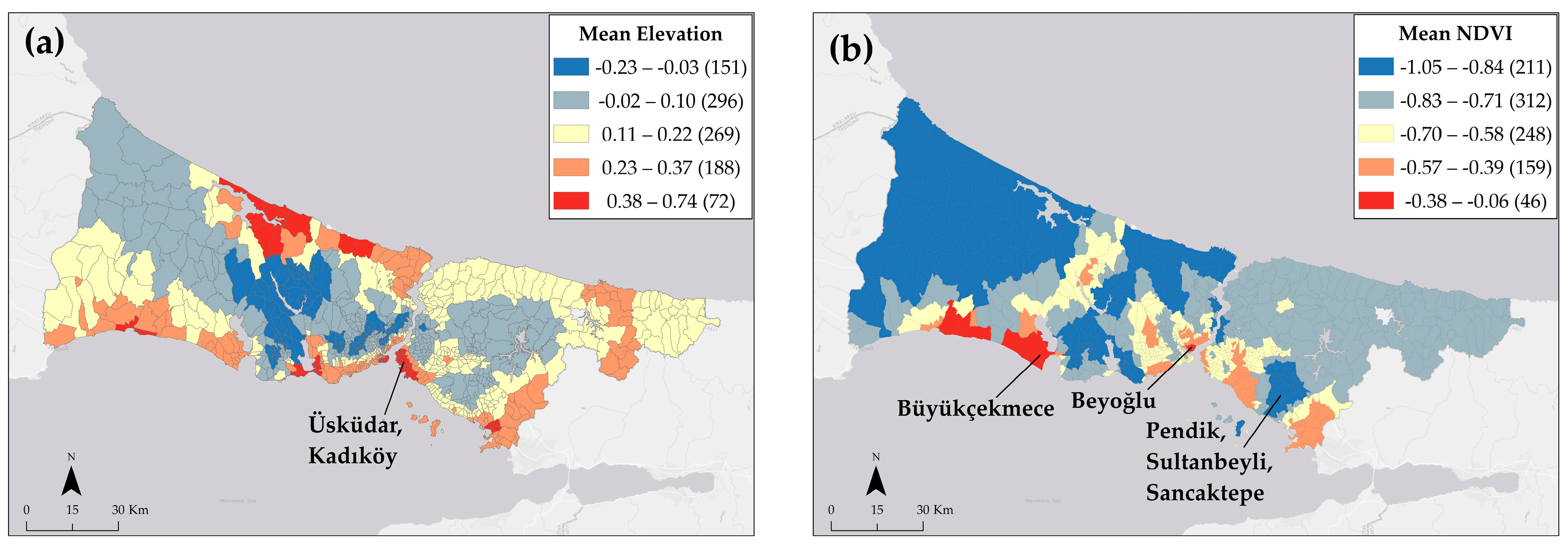
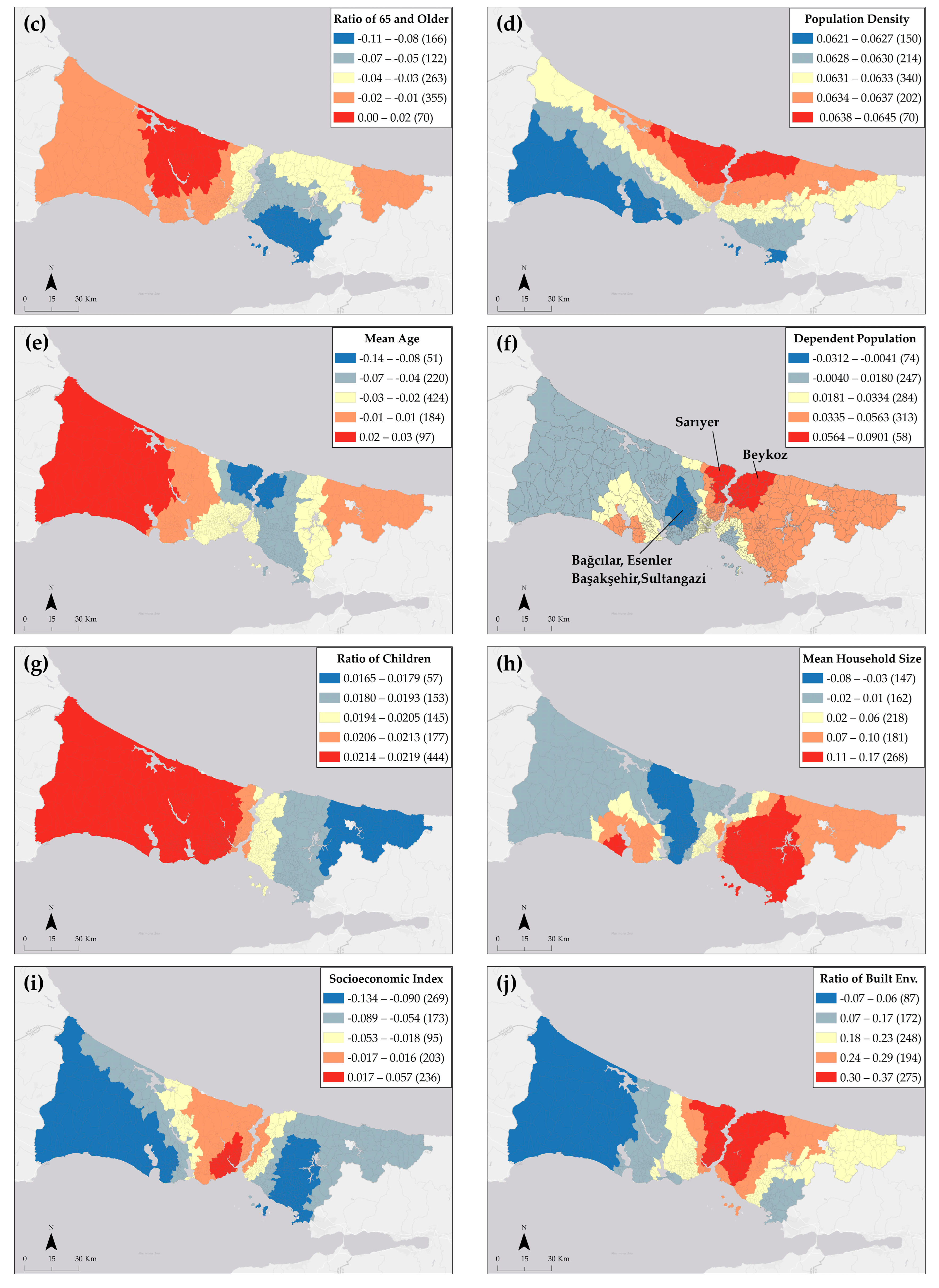
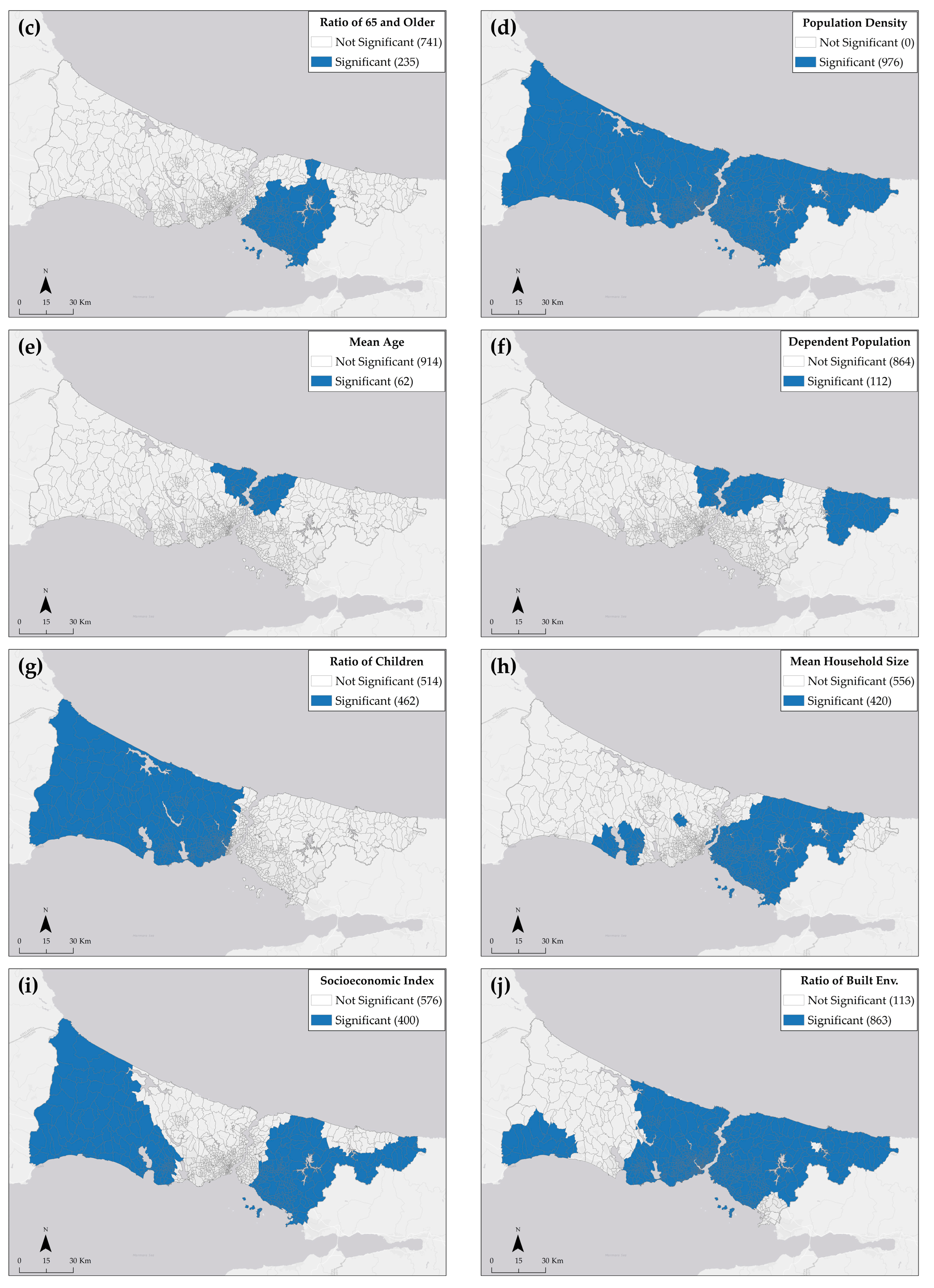
3.2. Spatial Model Results

The MGWR outperforms the GWR and OLS models with an adjusted R2 of 0.96.
This indicates that the inclusion of spatial structure takes into account previously unexplained variations. While the GWR considers fixed bandwidths for all neighborhoods, the MGWR bandwidth range varies between 30 and 976 (Table 3 and Table 4).
Under the geographically weighted framework, it is possible for collinearity to exist within local subsets [92]. Figure 4 displays the variability of local condition numbers (CN) for the GWR and MGWR models, even though there is no global presence of collinearity. This indicates that local collinearity diagnostic tests were employed in conjunction with the GWR and MGWR analyses. Collinearity significantly impacted some areas in the GWR model (most notably in the Bağcılar and Esenler counties). These numbers indicate a high degree of collinearity among the predictor variables [93]. The presence of collinearity in local subsets can be attributed to the fixed GWR bandwidth, as it can increase the collinearity between variables [89]. All of the local MGWR models exhibited condition numbers (CNs) below the threshold of 64.55.
Figure 4. Diagnostic tests of the local collinearity for the MGWR (a) and the GWR (b).
Sustainability 15 11594 g004
Figure 5 and Figure 6 show GWR and MGWR covariate coefficient estimates. Covariate coefficient estimates in the GWR and MGWR model turn from negative (blue) to positive (red), showing negative and positive relationships with land surface temperatures and socio-environmental variables. The relationship between LST and some variables can be completely negative or completely positive for Istanbul as a whole. In these maps, blue colors indicate neighborhoods where the relationship is weakened and red colors indicate neighborhoods where the relationship is strengthened (Figure 5 and Figure 6).
Figure 5. Spatial distribution of coefficients of GWR: mean elevation (a); mean NDVI (b); ratio of 65 and older (c); population density (d); mean age (e); dependent population (f); ratio of children (g); mean household size (h); socioeconomic index (i); ratio of built environment (j); total number of residences (k); intercept (l).
Sustainability 15 11594 g005aSustainability 15 11594 g005b
Figure 6. Spatial distribution of coefficients of MGWR: mean elevation (a); mean NDVI (b); ratio of 65 and older (c); population density (d); mean age (e); dependent population (f); ratio of children (g); mean household size (h); socioeconomic index (i); ratio of built environment (j); total number of residences (k); intercept (l).
Sustainability 15 11594 g006aSustainability 15 11594 g006bSustainability 15 11594 g006c
The coefficient estimates of the GWR model showed a positive relationship between LST and elevation on the southern coast of the European side (Zeytinburnu, Bakırköy). However, in the inner parts of both sides (Maltepe, Çekmeköy, Sultanbeyli, Arnavutköy), this relationship is negative. In the MGWR model, it was revealed that there is a positive relationship between LST and elevation in the southern coast of the European side and the south of Üsküdar and Kadıköy districts on the Asian side. GWR coefficient estimates show that there is a positive relationship between LST and mean NDVI in Üsküdar, Kadıköy, Beyoğlu, Şişli, and Fatih districts. In the MGWR model, the relationship is positive in Beyoğlu, Büyükçekmece, and Silivri districts.
According to the GWR model, there is a positive relationship between the ratio of 65 and older and the LST in 21 neighborhoods of Bağcılar and Esenler districts. Apart from that, the relationship is generally positive across the European side. MGWR coefficient estimates also show a positive relationship across the European side, and especially in the Arnavutköy district. In addition, MGWR showed that there is a negative relationship between the ratio of 65 and older and the LST in 166 neighborhoods in the southeast of the Asian side. According to the GWR coefficient estimates, there is a positive relationship between population density and LST in the west of the city. In the MGWR model, the relationship between the north of the city was positive. Generally, the relationship from north to south turns from positive to negative.
The coefficient estimates in the GWR model showed that there is a positive relationship between the LST and the mean age in Pendik, Kartal, and Bağcılar districts. In the MGWR model, on the other hand, this relationship was positive in the rural areas of Şile, Silivri, and Çatalca with low populations in the east and west, while a negative relationship was found in the urban areas where the mean age value was lower. It has been determined that the negative areas are clustered in the northern part of Bosphorus. According to the GWR coefficient estimates, there is a positive relationship between the dependent population and LST in Ataşehir, Ümraniye, Çekmeköy, and Sancaktepe districts. In the MGWR model, the relationship was positive in 58 neighborhoods in the north of the Bosphorus region (Beykoz, Sarıyer), while the relationship was negative in 74 neighborhoods in Bağcılar, Esenler, and Başakşehir.
The coefficient estimates of the GWR model showed that there is a positive relationship between LST and the ratio of children in Bağcılar, Bakırköy, Pendik, Tuzla, and Maltepe districts. In the MGWR model, it was observed that the relationship between LST and the ratio of children changed from positive to negative from west to east of the city. The GWR model showed that there is a positive relationship between LST and mean household size in some of the Beylikdüzü, Kadıköy, and Üsküdar districts. In addition, this relationship is negative in some of the districts of Küçükçekmece, Gaziosmanpaşa, and Sultangazi. MGWR coefficient estimates showed that there is a positive relationship between mean household size and LST in most of the Asian side (more than 200 neighborhoods).
GWR coefficient estimations showed that there is a positive relationship between the LST and the socioeconomic index in most of Şile and some of the districts of Kadıköy and Üsküdar. In Çekmeköy and Silivri, this relationship is generally negative. In the MGWR model, there is a positive relationship between LST and socioeconomic index in Fatih, Beyoğlu, Eyüpsultan, and Kağıthane districts. In general, the relationship turns from positive to negative as you move away from the Bosphorus region. GWR has shown that there is a positive relationship between the ratio of the built environment and LST in some of the districts of Üsküdar, Ataşehir, Maltepe, Kartal, Beykoz, and Sarıyer. Apart from this, the relationship was negative in the west of the European side and the eastern end of the Asian side. The MGWR coefficient estimates generally show that the relationship turns from positive to negative as you move away from the Bosphorus region. The coefficient estimates of the GWR model showed that there is a positive relationship between LST and the total number of residences in the Şile district. In 20 neighborhoods in the northwest corner of the city, this relationship is negative. The MGWR coefficient estimates generally show that the relationship from north to south turns from positive to negative.
The relationship between elevation and LST is significant mostly on the coasts, but it is also significant in the inner parts of districts, such as Tuzla and Şile. The relationship between mean NDVI and LST is significant in almost all of Istanbul. The relationship is not significant only in 26 neighborhoods on the coastline of the Büyükçekmece district. The relationship between the ratio of 65 and older and the LST is significant in most of the Asian side. The relationship between population density and LST is significant in Istanbul as a whole. The relationship between mean age and LST was significant in the north of Bosphorus. Similarly, the relationship between the dependent population and the LST is significant in the north of the Bosphorus and the Şile regions. The relationship between the ratio of children and the LST was significant in most of the European side (except for the Bosphorus region). The relationship between mean household size and LST is significant across the Asian side. The relationship between LST and socioeconomic index is significant in the west of the European side and east of the Asian side. The relationship between the ratio of the built environment and LST was significant in most of the urbanized areas (except Tuzla and Büyükçekmece). Finally, the relationship between the number of residences and LST was significant in 16 neighborhoods in the north of the city (Figure 7).
Figure 7. Spatial variation of p-values of MGWR models: mean elevation (a); mean NDVI (b); ratio of 65 and older (c); population density (d); mean age (e); dependent population (f); ratio of children (g); mean household size (h); socioeconomic index (i); ratio of built environment (j); total number of residences (k); intercept (l).
Sustainability 15 11594 g007aSustainability 15 11594 g007bSustainability 15 11594 g007c
In addition, the MGWR model extracts the relationships between variables in a scaled form. According to the results of the MGWR model, the relationships between the variables were determined together with the R2 values (Appendix A Table A1). As shown in Appendix A Table A1, strong relationships with an R2 value greater than 0.50 are between LST–mean NDVI, LST–ratio of the built environment, the ratio of built environment–mean NDVI, and built environment–population density. The R2 value of the relationships other than these is less than 0.10.

4. Discussion

In this study, three regression models were employed to explore the associations between land surface temperature and environmental and social factors, both in terms of aspatial and spatial distributions. We found that the LST in Istanbul is at higher levels outside the historical core, in rapidly urbanizing places, relatively lower socioeconomic levels, and densely populated peripheries. These regions are Sultanbeyli, Sancaktepe, and Ümraniye on the Asian side and Kağıthane, Eyüpsultan, Güngören, Bağcılar, Bahçelievler, and Esenyurt regions on the European side. The results show the variation in LST according to elevation, mean NDVI, the ratio of 65 and older, ratio of children, dependent population, population density, mean age, mean household size, the total number of residences, the ratio of the built environment, and socioeconomic index.

4.1. Social Determinants Association with LST

The relationship between the socioeconomic index and LST is negative in 66% of the neighborhoods. The relationship between LST and the socioeconomic index is positive in Fatih, Beyoğlu, Eyüpsultan, and Kağıthane regions. In general, the association turns positive to negative while moving away from the Bosphorus region. For example, Jenerette et al. [78] and Huang et al. [23] found a strong negative relationship between LST and socioeconomic levels in their study, where they used different methods in different American cities (Phoenix, AZ, USA and Baltimore, MD, USA).
Consistent with the literature [72,73,74], LST values increased in Istanbul as the population density increased. This positive relationship spread throughout the city. This positive relationship gets stronger from south to north. This finding can be explained by the fact that the south of the city is much more urbanized than the north.
The findings show that the relationship between the proportion of the population aged 65 and over and LST is negative in 95% of the neighborhoods. In this respect, the findings of the study are not consistent with the studies in the literature [75,76]. This negative relationship is stronger in 166 neighborhoods in the southeast of the Asian side. The significance map of the variable in Figure 7 is largely consistent with the neighborhoods where this relationship is negative. Moreover, in 62% of the neighborhoods where this relationship is negative, the relationship between LST and socioeconomic level is also negative. In other words, in almost two thirds of the city, LST decreases in neighborhoods where socioeconomic level and the proportion of the senior population increase. This finding is consistent with the results of the study conducted in Philadelphia [77]. In addition, the results show a positive relationship in general on the European side, especially in the Arnavutköy district. The Arnavutköy district is relatively outside the urban area of Istanbul. Compared to the city in general, Arnavutköy is a region where the population density and socioeconomic level are low, and the average NDVI value is high.
The findings show that the relationship between LST and children’s ratio varies positively throughout the city. This positive relationship gets stronger from east to west. Most of the 444 neighborhoods with high positive correlations are statistically significant in the significance map in Figure 6 and Figure 7 (See Figure 6 and Figure 7).
The findings show that there is a negative relationship between the proportion of the dependent population and LST. In 91% of the neighborhoods, this relationship is negative. The association between the dependent population and the LST is negative in 74 neighborhoods in Bağcılar, Esenler, and Başakşehir. However, in 58 neighborhoods (Beykoz, Sarıyer) in the northern part of Bosphorus, the relationship between the dependent population and LST was negative in 58 neighborhoods, as these 58 neighborhoods are greener and less built up.
The association between mean household size and LST differs across Istanbul. Neighborhoods where this relationship is positive are the majority with 72%. The relationship between mean household size and LST was found to be positive in most neighborhoods on the Asian side (more than 200 neighborhoods), as these neighborhoods are more urbanized. In most of the neighborhoods where this relationship is positive, the relationship between LST and socioeconomic index is negative. In other words, socioeconomic level decreases in neighborhoods where LST and household size increase. This finding is in line with the study conducted by Mashhoodi et al. [79] in the Netherlands. Apart from this, a negative relationship was found between LST and mean household size in the Bağcılar and Arnavutköy regions, where the average household size is higher than the city average.

4.2. Environmental Determinants Association with LST

The elevation estimates have a positive relationship with LST on the southern coast of the European side and south of Üsküdar and Kadıköy districts on the Asian side, as the south coasts are more built up [54] than the northern coasts. Accordingly, as the elevation increased, LST values decreased. For example, the study conducted by Liu et al. [27] reveals the negative relationship between elevation and LST for 252 of 323 cities distributed across the entire country of China. Similarly, Li et al. [20] found that increases in the elevation are associated with decreases in the LST in Shenzen, China.
The relationship between LST and NDVI is negative across the city. This finding is in line with the studies in the literature that investigated the relationship between NDVI and LST in different locations using different methods [19,22,27]. In some areas, this negative relationship weakens. The first of these is the Beyoğlu region. Beyoğlu, one of the historical cores of Istanbul, has a high density of built environment. There are fewer active green areas compared to other core regions such as Fatih. Therefore, this situation is expected. The second regions where the negative relationship weakens are Büyükçekmece and Silivri. The built environment ratio of these regions is much lower than Beyoğlu. Nevertheless, the reason for the weakening of this relationship may be the unused vacant land. In different studies in the literature, the LST averages of unused land are as high as those of high-density continuous urban and industrial areas [20,94,95]. As expected, the regions where the negative relationship is stronger are the forested areas in the north. However, this relationship is stronger in the northeast region.
The findings show that the relationship between the built environment and LST ratio generally turns positive to negative while moving away from the Bosphorus region. Neighborhoods where this relationship is positive are the majority with 94%. This result is consistent with the studies in the literature [20,28]. Additionally, in most of the neighborhoods (90%) where this relationship is positive, the relationship between LST and the socioeconomic index is negative. In other words, socioeconomic level decreases in neighborhoods where LST and built environment ratio increases. In addition, in most of the neighborhoods where this relationship is positive (98%), the relationship between LST and household size is positive. In other words, in neighborhoods where LST and built environment ratio increase, household size also increases.
Finally, it was found that the relationship between the total number of residences and LST, in general, turned from positive to negative from north to south. It is positive in the neighborhoods close to the northern coast of the Asian side. It is expected that the LST value will increase as the number of residences increases in these neighborhoods, where there are sparsely built 2-floor buildings [83].
ICV and ICCAP policy documents should be revised based on study findings. Trying to reduce the risks associated with extreme temperatures simply by planting trees in public areas is not an effective solution. With the findings of this study, which presents local variability for policy makers, the effectiveness of the planned actions should be tested with GIS-based 3D simulations. In urban transformation and urban planning processes, which come to the forefront due to earthquake risk, GIS-based 3D simulations related to the urban heat island should be made. In these simulations, trend analysis of meteorological stations, air pollution forecasts, fluid dynamics, urban geometry and typologies, traditional and innovative solutions, tree diversity, green roofs, solar power plants for roofs, reflective paint, and various architectural solutions should be considered. Through these simulations, the effectiveness of actions can be tested. In this way, neighborhood and street-specific actions can be planned. Incentives and penalties can be applied according to vulnerable groups and socioeconomic levels.
Indeed, the impacts of land surface temperature (LST) on sustainable development in mega cities like Istanbul are significant and multifaceted. Here are some key points to consider: 1. High LST in urban areas can lead to increased energy consumption for cooling, discomfort for residents, and adverse effects on human health while sustainable development goals prioritize reducing energy consumption and transitioning to cleaner and more efficient energy sources to mitigate climate change impacts; 2. By understanding the spatial variability of LST, city planners can identify areas prone to high temperatures and implement measures such as green spaces, urban parks, and tree planting to mitigate the UHI effect. Integrating sustainable design principles like green roofs, cool pavements, and efficient building materials can also help reduce LST and promote sustainable urban development; 3. LST influences water availability and quality in urban areas. Higher temperatures lead to increased water evaporation, stressing water resources. Sustainable water management practices, including water conservation, efficient irrigation systems, and green infrastructure for stormwater management, can help mitigate the impacts of LST on water resources and support sustainable urban development.

4.3. Limitations

This study has a few limitations. Since all the data used in the study were not produced yearly, a comparative study could not be conducted. Similarly, since not all data used in the study are produced annually, the latest and same-year data could not be used in this study. Therefore, it was necessary to choose years close to each other. Since the data forming the socioeconomic index could not be obtained, only income level or only education level variables could not be used in the model. The low temporal resolution of the Landsat images and the high cloudiness prevented the making of different LST maps. In addition, the absence of Landsat images at 10 pm, when the concrete surfaces give off the heat, limited comparisons within the same day. Unexpected results were obtained in some regions, as the shadows created by the skyscrapers reduced the LST values.

5. Conclusions

This study investigates the association between socioeconomic and environmental determinants and land surface temperature in Istanbul using spatial modeling methods. LST and covariates were analyzed using non-spatial OLS, as well as geographical GWR and MGWR models, to investigate their relationship accurately, considering both spatial and non-spatial aspects. The MGWR model outperforms the GWR model with an R2 of 0.96. In the GWR model, the use of a fixed bandwidth led to both overfitting and underfitting of variables, resulting in a misrepresentation of LST and its associations. To overcome this limitation, the MGWR model was selected.
The study advocates for multiscale and multidisciplinary policies and institutions to study LST association with socio-environmental determinants. Future studies should explore the non-linear association between LST and socio-environmental factors. In addition, nonlinear GWR approaches such as the geographically weighted artificial neural network (GWANN) and the geographically and temporally weighted neural network (GTWNN) can be tested in different seasons using methods such as reverse nearest neighbor (RNN), GWR, and 4D-GWR. Additionally, the combination of variables used in the study can be applied in different cities.
To address the impacts of LST on sustainable development in mega cities like Istanbul, a holistic and integrated approach is needed. This includes incorporating LST data into urban planning, adopting energy-efficient technologies, promoting green infrastructure, enhancing public health measures, and prioritizing climate change adaptation and mitigation strategies. By considering the relationship between LST and sustainable development, cities can work towards creating more resilient, livable, and sustainable urban environments.

Author Contributions

Conceptualization, Ö.Ü. and A.L.; methodology, Ö.Ü. and A.L.; software, Ö.Ü.; validation, Ö.Ü. and A.L.; formal analysis, Ö.Ü. and A.L.; investigation, Ö.Ü. and A.L.; resources, Ö.Ü. and A.L.; data curation, Ö.Ü.; writing—original draft preparation, Ö.Ü.; writing—review and editing, Ö.Ü., A.L. and S.A.; visualization, Ö.Ü.; supervision, A.L. and S.A.; project administration, Ö.Ü., A.L. and S.A.; funding acquisition, A.L. All authors have read and agreed to the published version of the manuscript.

Funding

This research received no external funding.

Institutional Review Board Statement

Not applicable.

Informed Consent Statement

Not applicable.

Data Availability Statement

Data will be provided upon reasonable request.

Conflicts of Interest

The authors declare no conflict of interest.

Appendix A

Table A1. Relationships between variables of MGWR models.
Variable 1Variable 2CorrelationPositive/NegativeChart
LSTMean NDVI0.76NegativeSustainability 15 11594 i001
LSTRatio of Built Environment0.58PositiveSustainability 15 11594 i002
LSTPopulation Density0.42PositiveSustainability 15 11594 i003
LSTTotal Number of Residences0.18PositiveSustainability 15 11594 i004
Total Number of ResidencesMean NDVI0.22NegativeSustainability 15 11594 i005
Ratio of Built EnvironmentMean NDVI0.71NegativeSustainability 15 11594 i006
Ratio of Built Env.Population Density0.61PositiveSustainability 15 11594 i007
Population DensityTotal Number of Residences0.26PositiveSustainability 15 11594 i008
Socioeco. IndexMean Elevation0.11NegativeSustainability 15 11594 i009
Socioeco. IndexRatio of 65 and older0.17PositiveSustainability 15 11594 i010
Ratio of ChildrenMean Age0.18NegativeSustainability 15 11594 i011
Ratio of ChildrenMean Household Size0.17PositiveSustainability 15 11594 i012

References

  1. Oke, T.R. Street design and urban canopy layer climate. Energy Build. 1988, 11, 103–113. [Google Scholar] [CrossRef]
  2. Yang, J.; Luo, X.; Jin, C.; Xiao, X.; Xia, J. Spatiotemporal patterns of vegetation phenology along the urban–rural gradient in Coastal Dalian, China. Urban For. Urban Green. 2020, 54, 126784. [Google Scholar] [CrossRef]
  3. British Columbia Coroners Service. Extreme Heat and Human Mortality: A Review of Heat-Related Deaths in B.C. in Summer 2021; British Columbia Coroners Service. 2022. Available online: https://www2.gov.bc.ca/assets/gov/birth-adoption-death-marriage-and-divorce/deaths/coroners-service/death-review-panel/extreme_heat_death_review_panel_report.pdf (accessed on 12 April 2023).
  4. Simon, F.; Lopez-Abente, G.; Ballester, E.; Martinez, F. Mortality in Spain during the heat waves of summer 2003. Eurosurveillance 2005, 10, 9–10. [Google Scholar] [CrossRef] [PubMed]
  5. Tobías, A.; Dominic, R.; Carmen, I. Heat-attributable Mortality in the Summer of 2022 in Spain. Epidemiology 2023, 34, e5–e6. [Google Scholar] [PubMed]
  6. Ellis, F.P.; Princé, H.P.; Lovatt, G.; Whittington, R.M. Mortality and Morbidity in Birmingham during the 1976 Heatwave. Qjm Int. J. Med. 1980, 49, 1–8. [Google Scholar] [CrossRef]
  7. Chien, L.C.; Guo, Y.; Zhang, K. Spatiotemporal analysis of heat and heat wave effects on elderly mortality in Texas, 2006–2011. Sci. Total Environ. 2016, 562, 845–851. [Google Scholar]
  8. Gürkan, H.; Eskioğlu, O.; Yazıcı, B.; Şensoy, S.; Kömüşçü, A.Ü.; Çalık, Y. Projected Trends in Heat and Cold Waves under Effect of Climate Change. In Proceedings of the 8th Atmospheric Sciences Symposium, Istanbul, Turkey, 1–4 November 2017. [Google Scholar]
  9. Erlat, E.; Türkeş, M.; Aydin-Kandemir, F. Observed changes and trends in heatwave characteristics in Turkey since 1950. Theor. Appl. Clim. 2021, 145, 137–157. [Google Scholar] [CrossRef]
  10. Unal, Y.S.; Tan, E.; Mentes, S.S. Summer heat waves over western Turkey between 1965 and 2006. Theor. Appl. Clim. 2013, 112, 339–350. [Google Scholar] [CrossRef]
  11. Amengual, A.; Homar, V.; Romero, R.; Brooks, H.; Ramis, C.; Gordaliza, M.; Alonso, S. Projections of heat waves with high impact on human health in Europe. Glob. Planet. Chang. 2014, 119, 71–84. [Google Scholar] [CrossRef]
  12. Perkins, S.E.; Alexander, L.V.; Nairn, J.R. Increasing frequency, intensity and duration of observed global heatwaves and warm spells. Geophys. Res. Lett. 2012, 39, 10. [Google Scholar]
  13. Hou, K.; Zhang, L.; Xu, X.; Yang, F.; Chen, B.; Hu, W.; Shu, R. High ambient temperatures are associated with urban crime risk in Chicago. Sci. Total. Environ. 2023, 856, 158846. [Google Scholar] [PubMed]
  14. Anderson, C.A.; Delisi, M. Implications of Global Climate Change for Violence in Developed and Developing Countries. In The Psychology of Social Conflict and Aggression; Forgas, J., Kruglanski, A., Williams, K., Eds.; Psychology Press: New York, NY, USA, 2011; pp. 249–265. [Google Scholar]
  15. McDowall, D.; Loftin, C.; Pate, M. Seasonal cycles in crime, and their variability. J. Quant. Criminol. 2012, 28, 389–410. [Google Scholar]
  16. Zander, K.K.; Botzen, W.J.W.; Oppermann, E.; Kjellstrom, T.; Garnett, S.T. Heat stress causes substantial labour productivity loss in Australia. Nat. Clim. Chang. 2015, 5, 647–651. [Google Scholar] [CrossRef]
  17. Lundgren, K.; Kuklane, K.; Gao, C.; Holmer, I. Effects of heat stress on working populations when facing climate change. Ind. Health 2013, 51, 3–15. [Google Scholar]
  18. Mashhoodi, B. Environmental justice and surface temperature: Income, ethnic, gender, and age inequalities. Sustain. Cities Soc. 2021, 68, 102810. [Google Scholar]
  19. Xian, G.; Crane, M. An analysis of urban thermal characteristics and associated land cover in Tampa Bay and Las Vegas using Landsat satellite data. Remote Sens. Environ. 2006, 104, 147–156. [Google Scholar]
  20. Li, S.; Zhao, Z.; Miaomiao, X.; Wang, Y. Investigating spatial non-stationary and scale-dependent relationships between urban surface temperature and environmental factors using geographically weighted regression. Environ. Model. Softw. 2010, 25, 1789–1800. [Google Scholar]
  21. Ivajnšič, D.; Kaligarič, M.; Žiberna, I. Geographically weighted regression of the urban heat island of a small city. Appl. Geogr. 2014, 53, 341–353. [Google Scholar] [CrossRef]
  22. Bokaie, M.; Zarkesh, M.K.; Arasteh, P.D.; Hosseini, A. Assessment of Urban Heat Island based on the relationship between land surface temperature and Land Use/Land Cover in Tehran. Sustain. Cities Soc. 2016, 23, 94–104. [Google Scholar]
  23. Huang, G.; Zhou, W.; Cadenasso, M.L. Is everyone hot in the city? Spatial pattern of land surface temperatures, land cover and neighborhood socioeconomic characteristics in Baltimore, MD. J. Environ. Manag. 2011, 92, 1753–1759. [Google Scholar]
  24. He, J.; Zhao, W.; Li, A.; Wen, F.; Yu, D. The impact of the terrain effect on land surface temperature variation based on Landsat-8 observations in mountainous districts. Int. J. Remote Sens. 2018, 40, 1808–1827. [Google Scholar]
  25. Guo, A.; Yang, J.; Sun, W.; Xiao, X.; Cecilia, J.X.; Jin, C.; Li, X. Impact of urban morphology and landscape characteristics on spatiotemporal heterogeneity of land surface temperature. Sustain. Cities Soc. 2020, 63, 102443. [Google Scholar] [CrossRef]
  26. Gao, S.; Zhan, Q.; Yang, C.; Liu, H. The Diversified Impacts of Urban Morphology on Land Surface Temperature among Urban Functional Zones. Int. J. Environ. Res. Public Health 2020, 17, 9578. [Google Scholar] [CrossRef] [PubMed]
  27. Liu, H.; Huang, B.; Gao, S.; Wang, J.; Yang, C.; Li, R. Impacts of the evolving urban development on intra-urban surface thermal environment: Evidence from 323 Chinese cities. Sci. Total. Environ. 2021, 771, 144810. [Google Scholar] [PubMed]
  28. Xiao, R.; Weng, Q.; Ouyang, Z.; Li, W.; Schienke, E.W.; Zhang, Z. Land Surface Temperature Variation and Major Factors in Beijing, China. Photogramm. Eng. Remote Sens. 2008, 74, 451–461. [Google Scholar] [CrossRef] [Green Version]
  29. Yang, L.; Yu, K.; Ai, J.; Liu, Y.; Yang, W.; Liu, J. Dominant Factors and Spatial Heterogeneity of Land Surface Temperatures in Urban Areas: A Case Study in Fuzhou, China. Remote Sens. 2022, 14, 1266. [Google Scholar]
  30. Toros, H.; Abbasnia, M.; Sagdic, M.; Tayanç, M. Long-Term Variations of Temperature and Precipitation in the Megacity of Istanbul for the Development of Adaptation Strategies to Climate Change. Adv. Meteorol. 2017, 2017, 6519856. [Google Scholar] [CrossRef] [Green Version]
  31. Doğan, T.; Hanel, M.; Oğuz, K.; Demircan, M. Assessment of The Urban Heat Island Effect Under Current and Climate Change Conditions in Istanbul. In Proceedings of the International Multidisciplinary Scientific GeoConference, Albena, Bulgaria, 28 June–7 July 2019. [Google Scholar]
  32. World Bank Group. Türkiye Country Climate and Development Report; World Bank: Washington, DC, USA, 2022. [Google Scholar]
  33. IPCC. Climate Change 2022: Impacts, Adaptation and Vulnerability. Contribution of Working Group II to the Sixth Assessment Report of the Intergovernmental Panel on Climate Change; Cambridge University Press: Cambridge, UK; New York, NY, USA, 2022. [Google Scholar]
  34. Çulpan, H.C.; Şahin; Can, G. A Step to Develop Heat-Health Action Plan: Assessing Heat Waves’ Impacts on Mortality. Atmosphere 2022, 13, 2126. [Google Scholar]
  35. Can, G.; Şahin, Ü.; Sayılı, U.; Dubé, M.; Kara, B.; Acar, H.C.; İnan, B.; Sayman, A.; Lebel, G.; Bustinza, R.; et al. Excess Mortality in Istanbul during Extreme Heat Waves between 2013 and 2017. Int. J. Environ. Res. Public Health 2019, 16, 4348. [Google Scholar]
  36. Karaca, M.; Tayanç, M.; Toros, H. Effects of urbanization on climate of İstanbul and Ankara. Atmos. Environ. 1995, 29, 3411–3421. [Google Scholar]
  37. Karaca, M.; Anteplioğlu, Ü.; Karsan, H. Detection of urban heat island in Istanbul, Turkey. II Nuovo C. C 1995, 18, 49–55. [Google Scholar]
  38. Dihkan, M.; Karsli, F.; Guneroglu, A.; Guneroglu, N. Evaluation of surface urban heat island (SUHI) effect on coastal zone: The case of Istanbul Megacity. Ocean Coast. Manag. 2015, 118, 309–316. [Google Scholar]
  39. Ünal, Y.S.; Sonuç, C.Y.; İncecik, S.; Topçu, H.S.; Diren-Üstün, D.H.; Temizöz, H.P. Investigating urban heat island intensity in Istanbul. Theor. Appl. Climatol. 2019, 139, 175–190. [Google Scholar]
  40. Khorrami, B.; Gunduz, O. Spatio-temporal interactions of surface urban heat island and its spectral indicators: A case study from Istanbul metropolitan area, Turkey. Environ. Monit. Assess. 2020, 192, 386. [Google Scholar]
  41. Aksak, P.; Öztürk, Ş.K.; Ünsal, Ö. Investigation of Urban Heat Island Effect on Climate Parameters and Remote Sensing: The Case of Istanbul City. Aegean Geogr. J. 2023, 32, 151–171. [Google Scholar]
  42. Okumus, D.E.; Terzi, F. Reconsidering Urban Densification for Microclimatic Improvement: Planning and Design Strategies for Istanbul. Iconarp Int. J. Arch. Plan. 2022, 10, 660–687. [Google Scholar]
  43. Okumus, D.E.; Terzi, F. Evaluating the role of urban fabric on surface urban heat island: The case of Istanbul. Sustain. Cities Soc. 2021, 73, 103128. [Google Scholar]
  44. Istanbul Metropolitan Municipality. Istanbul Climate Vision; Istanbul Metropolitan Municipality: Istanbul, Turkey, 2021. [Google Scholar]
  45. Istanbul Metropolitan Municipality. Istanbul Climate Change Action Plan; Istanbul Metropolitan Municipality: Istanbul, Turkey, 2021. [Google Scholar]
  46. Bölen, F.; Türkeroğlu, H.E.; Ergün, N.; Yirmibeşoğlu, F.; Terzi, F.; Kaya, S.; Kundak, S. Quality of Residential Environment in a City Facing Unsustainable Growth Problems: Istanbul. In Proceedings of the New Approaches in Urban and Regional Planning, Istanbul, Turkey, 28–29 April 2008. [Google Scholar]
  47. Turkish Statistical Institute. Central Dissemination System. 2023. Available online: https://biruni.tuik.gov.tr/medas/?locale=en (accessed on 7 January 2023).
  48. UN. Transforming Our World: The 2030 Agenda for Sustainable Development; United Nations: New York, NY, USA, 2015. [Google Scholar]
  49. UN. World Urbanization Prospects: The 2018 Revision; United Nations: New York, NY, USA, 2019. [Google Scholar]
  50. Istanbul Metropolitan Municipality. 2023. Available online: https://www.ibb.istanbul/en (accessed on 5 January 2023).
  51. Avcı, S. Population Characteristics of Istanbul and Vulnerability to Disasters. In Proceedings of the Istanbul’s Disaster Vulnerability Symposium, Istanbul, Turkey, 4–5 October 2010. [Google Scholar]
  52. Terzi, F.; Bölen, F. The Potential Effects of Spatial Strategies on Urban Sprawl in Istanbul. Urban Stud. 2011, 49, 1229–1250. [Google Scholar]
  53. Terzi, F.; Bolen, F. Urban Sprawl Measurement of Istanbul. Eur. Plan. Stud. 2009, 17, 1559–1570. [Google Scholar]
  54. Geymen, A.; Baz, I. Monitoring urban growth and detecting land-cover changes on the Istanbul metropolitan area. Environ. Monit. Assess. 2007, 136, 449–459. [Google Scholar]
  55. Dereli, M.A. Monitoring and prediction of urban expansion using multilayer perceptron neural network by remote sensing and GIS technologies: A case study from Istanbul Metropolitan City. Fresenius Environ. Bull. 2018, 27, 9336–9344. [Google Scholar]
  56. Öztürk, M.Z.; Çetinkaya, G.; Aydın, S. Climate Types of Turkey According to Köppen-Geiger Climate Classification. J. Geogr. 2017, 35, 17–27. [Google Scholar]
  57. Yılmaz, E.; Çiçek, İ. Türkiye’nin detaylandırılmış Köppen-Geiger iklim bölgeleri. J. Hum. Sci. 2018, 15, 225–242. [Google Scholar]
  58. Türkeş, M. Climate and Drought in Turkey. In Water Resources of Turkey; Harmancıoğlu, N.B., Altınbilek, D., Eds.; Springer: Cham, Switzerland, 2020; pp. 85–125. [Google Scholar] [CrossRef]
  59. Turoğlu, H. Detection of Changes on Temperature and Precipitation Features in Istanbul (Turkey). Atmos. Clim. Sci. 2014, 4, 549–562. [Google Scholar]
  60. Ezber, Y.; Şen, Ö.L.; Kındap, T.; Karaca, M. Climatic effects of urbanization in Istanbul: A statistical and modeling analysis. Int. J. Climatol. 2006, 27, 667–679. [Google Scholar]
  61. Avdan, U.; Jovanovska, G. Algorithm for Automated Mapping of Land Surface Temperature Using LANDSAT 8 Satellite Data. J. Sens. 2016, 2016, 1480307. [Google Scholar]
  62. Chander, G.; Markham, B. Revised landsat-5 tm radiometric calibration procedures and postcalibration dynamic ranges. IEEE Trans. Geosci. Remote Sens. 2003, 41, 2674–2677. [Google Scholar]
  63. Coll, C.; Galve, J.M.; Sánchez, J.M.; Caselles, V. Alidation of Landsat-7/ETM+ thermal band calibration and atmospheric correction with ground-based measurements. IEEE Trans. Geosci. Remote Sens. 2010, 48, 547–555. [Google Scholar]
  64. USGS. Using the USGS Landsat Level-1 Data Product. 2021. Available online: https://www.usgs.gov/landsat-missions/using-usgs-landsat-level-1-data-product (accessed on 24 November 2022).
  65. Tucker, C.J. Red and photographic infrared linear combinations for monitoring vegetation. Remote Sens. Environ. 1979, 8, 127–150. [Google Scholar]
  66. Sobrino, J.A.; Jiménez-Muñoz, J.C.; Paolini, L. Land surface temperature retrieval from LANDSAT TM 5. Remote Sens. Environ. 2004, 90, 434–440. [Google Scholar]
  67. Sobrino, J.A.; Jimenez-Munoz, J.C.; Soria, G.; Romaguera, M.; Guanter, L.; Moreno, J.; Plaza, A.; Martinez, P. Land Surface Emissivity Retrieval from Different VNIR and TIR Sensors. IEEE Trans. Geosci. Remote Sens. 2008, 46, 316–327. [Google Scholar] [CrossRef]
  68. Fisher, W.D. On Grouping for Maximum Homogeneity. J. Am. Stat. Assoc. 1958, 53, 789–798. [Google Scholar] [CrossRef]
  69. Jenks, G.; Caspall, F. Error on Choropleth Maps: Definition, Measurement, Reduction. Ann. Assoc. Am. Geogr. 1971, 61, 217–244. [Google Scholar] [CrossRef]
  70. Murray, A.T.; Shyy, T.-K. Integrating attribute and space characteristics in choropleth display and spatial data mining. Int. J. Geogr. Inf. Sci. 2000, 14, 649–667. [Google Scholar] [CrossRef]
  71. De Smith, M.J.; Goodchild, M.F.; Longley, P.A. Geospatial Analysis: A Comprehensive Guide to Principles, Techniques and Software Tools, 6th ed.; The Winchelsea Press: London, UK, 2018. [Google Scholar]
  72. Weng, Q.; Liu, H.; Liang, B.; Lu, D. The Spatial Variations of Urban Land Surface Temperatures: Pertinent Factors, Zoning Effect, and Seasonal Variability. IEEE J. Sel. Top. Appl. Earth Obs. Remote Sens. 2008, 1, 154–166. [Google Scholar] [CrossRef]
  73. Kotharkar, R.; Surawar, M. Land Use, Land Cover, and Population Density Impact on the Formation of Canopy Urban Heat Islands through Traverse Survey in the Nagpur Urban Area, India. J. Urban Plan. Dev. 2016, 142, 04015003. [Google Scholar] [CrossRef]
  74. Huang, G.; Cadenasso, M.L. People, landscape, and urban heat island: Dynamics among neighborhood social conditions, land cover and surface temperatures. Landsc. Ecol. 2016, 31, 2507–2515. [Google Scholar] [CrossRef]
  75. Hulley, G.; Shivers, S.; Wetherley, E.; Cudd, R. New ECOSTRESS and MODIS Land Surface Temperature Data Reveal Fine-Scale Heat Vulnerability in Cities: A Case Study for Los Angeles County, California. Remote Sens. 2019, 11, 2136. [Google Scholar] [CrossRef] [Green Version]
  76. Kenny, G.P.; Yardley, J.; Brown, C.; Sigal, R.J.; Jay, O. Heat stress in older individuals and patients with common chronic diseases. Can. Med. Assoc. J. 2009, 182, 1053–1060. [Google Scholar] [CrossRef] [Green Version]
  77. Johnson, D.P.; Wilson, J.S. The socio-spatial dynamics of extreme urban heat events: The case of heat-related deaths in Philadelphia. Appl. Geogr. 2009, 29, 419–434. [Google Scholar] [CrossRef]
  78. Jenerette, G.D.; Harlan, S.L.; Brazel, A.; Jones, N.; Larsen, L.; Stefanov, W.L. Regional relationships between surface temperature, vegetation, and human settlement in a rapidly urbanizing ecosystem. Landsc. Ecol. 2007, 22, 353–365. [Google Scholar] [CrossRef]
  79. Mashhoodi, B.; Stead, D.; van Timmeren, A. Land surface temperature and households’ energy consumption: Who is affected and where? Appl. Geogr. 2019, 114, 102125. [Google Scholar] [CrossRef]
  80. Şeker, M.; Ersöz, H.Y.; Kazan, H.; Saldanlı, A.; Akman, S.U.; Bektaş, H.; Şişmanoğlu, E.; Yurduer, Y.; Uzun, S. Mahallem Istanbul Project; Istanbul University: Istanbul, Turkey, 2017. [Google Scholar]
  81. GEE. Google Earth Engine. 2023. Available online: https://earthengine.google.com (accessed on 10 September 2022).
  82. Copernicus, EU-DEM. 2016. Available online: https://land.copernicus.eu/imagery-in-situ/eu-dem/eu-dem-v1.1 (accessed on 24 September 2022).
  83. DB, Urban Atlas. Available online: https://www.csb.gov.tr (accessed on 24 December 2022).
  84. Rogerson, P.A. Data reduction: Factor analysis and cluster analysis. Stat. Methods Geogr. 2001, 2001, 192–197. [Google Scholar]
  85. Haining, R.P. Spatial Sampling. Int. Encycl. Soc. Behav. Sci. 2001, 14822–14827. [Google Scholar] [CrossRef]
  86. Paul, R.; Voss, K.J.; Curtis, W.; Roger, B.H. Explorations in Spatial Demography. In Population Change and Rural Society; Kandel, W.A., Brown, D.L., Eds.; Springer: Berlin/Heidelberg, Germany, 2006; pp. 407–429. [Google Scholar]
  87. Fotheringham, A.S.; Brunsdon, C.; Charlton, M. Geographically Weighted Regression: The Analysis of Spatially Varying Relationships; Wiley: Hoboken, NJ, USA, 2002. [Google Scholar]
  88. Lotfata, A. Using Geographically Weighted Models to Explore Obesity Prevalence Association with Air Temperature, Socioeconomic Factors, and Unhealthy Behavior in the USA. J. Geovisualization Spat. Anal. 2022, 6, 14. [Google Scholar] [CrossRef]
  89. Oshan, T.M.; Fotheringham, A.S. A Comparison of Spatially Varying Regression Coefficient Estimates Using Geographically Weighted and Spatial-Filter-Based Techniques. Geogr. Anal. 2017, 50, 53–75. [Google Scholar] [CrossRef]
  90. Yilmaz, M.; Hamurcu, A.U. Relationships between socio-demographic structure and spatio-temporal distribution patterns of COVID-19 cases in Istanbul, Turkey. Int. J. Urban Sci. 2022, 26, 557–581. [Google Scholar] [CrossRef]
  91. Oshan, T.M.; Li, Z.; Kang, W.; Wolf, L.J.; Fotheringham, A.S. mgwr: A Python Implementation of Multiscale Geographically Weighted Regression for Investigating Process Spatial Heterogeneity and Scale. ISPRS Int. J. Geo Inf. 2019, 8, 269. [Google Scholar] [CrossRef] [Green Version]
  92. Wheeler, D.; Tiefelsdorf, M. Multicollinearity and correlation among local regression coefficients in geographically weighted regression. J. Geogr. Syst. 2005, 7, 161–187. [Google Scholar] [CrossRef]
  93. Gollini, I.; Lu, B.; Charlton, M.; Brunsdon, C.; Harris, P. GWmodel: An R package for exploring spatial heterogeneity using geographically weighted models. J. Stat. Softw. 2015, 63, 1–50. [Google Scholar] [CrossRef] [Green Version]
  94. Ünsal; Avci, V. Determining the Relationship Between Land Surface Temperatures and Urban Land Use: The Example of Şanlıurfa, Diyarbakır and Mardin. Turk. J. Remote Sens. GIS 2023, 4. [Google Scholar]
  95. Ünsal; Kuzulugil, A.C.; Aytatlı, B.; Demircioğlu Yıldız, N. Determining the Change of Land Use Types by Years with Land Surface Temperature Data (Erzurum City Case Study). J. Urban Cult. Manag. 2023, 16, 1334–1361. [Google Scholar]
Figure 1. Study area.
Sustainability 15 11594 g001
Figure 2. Mean LST of Istanbul neighborhoods.
Sustainability 15 11594 g002
Table 1. Explanation of covariates.
CovariateUnitSourceCalculation Method
Mean ElevationMeterEU DEM v1.1Downloaded from EU DEM v1.1, used zonal statistics by neighborhood
Mean NDVIIndex GEE Downloaded from GEE, used zonal statistics by neighborhood
Ratio of 65 and Older%TSI + IMMDivided +65 aged population to total population by neighborhood
Population DensityPerson/km2TSI + IMMDivided total population into neighborhood area
Mean AgeValueTSI + IMMObtained from IMM by neighborhood directly
Dependent PopulationIndexTSI + IMMDivided +65 and 0–15 aged population to total population by neighborhood
Ratio of Children%TSI + IMMDivided 0–18 aged population to total population by neighborhood
Mean Household SizeIndexTSI + IMMObtained from IMM by neighborhood directly
Socioeconomic IndexIndexMahallem Istanbul ProjectObtained from Mahallem Istanbul Project report file by neighborhood directly
Ratio of Built Environment%Ministry of Environment, Urbanization, and Climate Change The total area of impermeable surfaces of urban atlas by neighborhood
Total Number of ResidencesValueIMMObtained from IMM by neighborhood directly
Table 2. OLS results.
VariableCoefficientStd. Errort-Statisticp-ValueVIF
Intercept33.890.4869.850.00-
Mean Elevation0.010.0018.980.001.39
Mean NDVI −22.980.69−33.200.004.84
Ratio of 65 and older0.700.740.940.001.46
Population Density0.000.003.730.003.36
Mean Age0.010.002.440.031.58
Dependent Population0.500.281.750.001.39
Ratio of Children0.080.024.000.001.81
Mean Household Size1.430.314.500.021.43
Socioeconomic Index−0.010.00−5.490.001.64
Ratio of Built Environment0.010.003.180.006.40
Total Number of Residences−0.010.00−1.960.001.58
Adjusted R20.86
AICc2978.60
Table 3. GWR and MGWR model results.
StatisticGWR ResultsMGWR Results
Adjusted R20.950.96
AICc2210.98−242.32
Sigma-squared0.420.03
Sigma-squared MLE0.290.02
Effective degrees of freedom671.88759.26
Table 4. Summary statistics for MGWR parameter estimates.
Bandwidth
(% of Features)
Significant
(% of Features)
MeanStd. Dev.MinMedianMax
Intercept31 (3.18)274 (28.07)0.060.16−0.440.060.43
Mean Elevation30 (3.01)343 (35.14)0.120.15−0.230.110.74
Mean NDVI 30 (3.07)950 (97.34)−0.690.17−1.05−0.71−0.05
Ratio of 65 and older391 (40.06)235 (24.08)−0.040.03−0.11−0.320.02
Population Density306 (31.35)976 (100)0.050.030.010.040.12
Mean Age391 (40.06)62 (6.35)−0.020.02−0.13−0.030.02
Dependent Population306 (31.35)112 (11.48)0.020.02−0.030.020.09
Ratio of Children976 (100)462 (47.34)0.020.000.010.020.02
Mean Household Size173 (17.73)420 (43.03)0.040.06−0.080.040.17
Socioeconomic Index201 (20.59)400 (40.98)−0.030.05−0.13−0.030.05
Ratio of Built Environment165 (16.91)863 (88.42)0.210.09−0.070.220.36
Total Number of Residences976 (100)16 (1.64)0.000.000.000.000.00
Disclaimer/Publisher’s Note: The statements, opinions and data contained in all publications are solely those of the individual author(s) and contributor(s) and not of MDPI and/or the editor(s). MDPI and/or the editor(s) disclaim responsibility for any injury to people or property resulting from any ideas, methods, instructions or products referred to in the content.

