Article

Smart Agricultural–Industrial Crop-Monitoring System Using Unmanned Aerial Vehicle–Internet of Things Classification Techniques

1
Department of Computational Intelligence, School of Computing, SRM Institute of Science and Technology, College of Engineering and Technology, Kattankulathur, Chennai 603203, Tamil Nadu, India
2
Department of Information Systems, College of Computer and Information Sciences, Princess Nourah Bint Abdulrahman University, Riyadh 11671, Saudi Arabia
3
Department of CSE, Koneru Lakshmaiah Education Foundation, Vaddeswaram 522502, Andhra Pradesh, India
4
Faculty of Information Technology, Applied Science Private University, Amman 11931, Jordan
5
Department of Computer Networks, College of Computer Sciences and Information Technology, King Faisal University, Al-Ahsa 31982, Saudi Arabia
6
Institute of Computer Science and Engineering, Saveetha School of Engineering, Saveetha Institute of Medical and Technical Sciences, Chennai 602105, Tamil Nadu, India
7
Department of EEE, Dhanalakshmi Srinivasan College of Engineering, Coimbatore 641105, Tamilnadu, India
8
Management Department, College of Business Administration, Ajman University, Ajman 346, United Arab Emirates
*
Author to whom correspondence should be addressed.
Sustainability 2023, 15(14), 11242; https://doi.org/10.3390/su151411242
Submission received: 23 May 2023 / Revised: 6 July 2023 / Accepted: 12 July 2023 / Published: 19 July 2023
(This article belongs to the Special Issue Sustainable Information Engineering and Computer Science)

Abstract

:
Unmanned aerial vehicles (UAVs) coupled with machine learning approaches have attracted considerable interest from academicians and industrialists. UAVs provide the advantage of operating and monitoring actions performed in a remote area, making them useful in various applications, particularly the area of smart farming. Even though the expense of controlling UAVs is a key factor in smart farming, this motivates farmers to employ UAVs while farming. This paper proposes a novel crop-monitoring system using a machine learning-based classification with UAVs. This research aims to monitor a crop in a remote area with below-average cultivation and the climatic conditions of the region. First, data are pre-processed via resizing, noise removal, and data cleaning and are then segmented for image enhancement, edge normalization, and smoothing. The segmented image was pre-trained using convolutional neural networks (CNN) to extract features. Through this process, crop abnormalities were detected. When an abnormality in the input data is detected, then these data are classified to predict the crop abnormality stage. Herein, the fast recurrent neural network-based classification technique was used to classify abnormalities in crops. The experiment was conducted by providing the present weather conditions as the input values; namely, the sensor values of temperature, humidity, rain, and moisture. To obtain results, around 32 truth frames were taken into account. Various parameters—namely, accuracy, precision, and specificity—were employed to determine the accuracy of the proposed approach. Aerial images for monitoring climatic conditions were considered for the input data. The data were collected and classified to detect crop abnormalities based on climatic conditions and pre-historic data based on the cultivation of the field. This monitoring system will differentiate between weeds and crops.

1. Introduction

Farmers use herbicides to maintain and ensure the quantity and quality of producing crops. Generally, herbicides are distributed completely over fields, even in weed-free areas, as weeds may be distributed spatially in some areas [1]. Recently, expected yields have not been obtained because of weeds. Moreover, economic and environmental risks occur and have led various polities and countries (Europe, Australia, Brazil, and the USA) to create legislation for the justifiable use of pesticides and provided guidelines to reduce the use of chemicals [2]. According to these guidelines, spraying area-wise is permitted in site-specific weed management (SSWM) based on weed coverage. One way to ensure SSWM earlier is to use precise weed maps appropriately to monitor post-emergence weeds. So far, monitoring weeds is performed either by detecting them remotely or via ground sampling. In this study, remote sensing was used to significantly improve the reliability of SSWM for suitable spatial and spectral resolutions in order to distinguish spectral reflectance [3]. However, some appearance features of multiple crops, as well as weeds, are identical in the earliest stage of growth. To find a solution for this, a few works have mapped weeds at later stages than the earliest growth stages. However, as spatial resolution is scarce, these techniques have not been applied successfully for detection at earlier stages. But recently, a novel aerial technique was integrated with existing techniques, namely, unmanned aerial vehicles (UAVs) [4]. Machine learning and image analysis have been utilized for precision cultivation with UAV imagery in a few recent projects, and this is a growing field (despite its limitations). Based on this, a common way to design an organization scheme for weeds that involves UAVs is to use rules that are manually defined based on differences in the spectra, location, and indexes of vegetation. However, it is believed that remote sensing provides advantages, to some extent, over other image analyzing and machine learning approaches. Such methods have successfully employed on-the-ground images to motivate further research works in this area, but a few limitations have been found regarding proximal sensing, which make it difficult to use these techniques practically in real-time applications [5]. Conversely, remote sensing has to be performed beforehand and helps determine whether herbicides are needed, thus optimizing the target field. This was an issue recently found in UAVs, but this is considered an acceptable cost. Several studies have presented the benefits and feasibility of UAVs and, thus, have developed novel approaches to monitoring the growth of weeds, testing them with various experimental setups. UAVs focus on vertical applications with no consideration of issues in particular vertical domains or across application domains. Moreover, practical ways to overcome these issues have not been discussed.
In [6,7], the features and demands for UAV networks for civil applications were presented by considering their communication and networking aspects. Requirements like the quality of service, parameters related to the network, data, and the minimal transmission of data through the network for civil applications were examined. Moreover, the requirements for general networking, namely, adaptability, connectivity, security, privacy, and scalability, were also discussed. Finally, suitable communication technology was identified to support reliable aerial networks. The research in [8] focused on routing and energy efficiency. First, infrastructure and an ad hoc UAV network were designed concerning a particular area of application, wherein a UAV acted as a server or client with a mesh or star UAV network, identifying difficulties in deployment disruptions and delays. Then, routing issues, as well as the energy efficiency of the UAV networks, were examined. In [9], flying ad hoc networks (FANETs) connected to UAVs were examined. First, the functions of FANETs, vehicle ad hoc networks (VANETs), and mobile ad hoc networks (MANETs) were studied. Then, the challenges of using FANETs were discussed. In [10], an overview of UAV-aided wireless communication was presented by deploying a basic network architecture. The authors focused on key designs, and opportunities were discovered.
In [11], an introduction to the history and the development of public safety communication techniques, as well as the use of spectral allotment for public safety use, with all sorts of frequencies was discussed. It was concluded that UAV applications supporting public safety communications were covered by privacy factors and there was a lack of comprehensive rules and regulations, policies, and management of UAVs. In [12], cooperative swarm UAVs applications, which acted as a distributed processing system, were described. Distributed processing applications were further classified as general-purpose applications, object-detecting applications, tracking applications, surveillance applications, applications collecting data, applications for path planning, navigating applications, applications for collision avoidance, coordinating applications, and applications that monitor the environment. But an issue faced by these applications was not taken into consideration. A comprehensive survey was provided in [13] on UAVs, focusing on their usage in the delivery of the Internet of Things (IoT). The architecture for UAVs with related key challenges and needs was discussed. Figure 1 below shows the sample images of sample crops and few common weeds identified the field.
Even though UAV imaging is of great use, its technologies have numerous practical challenges. At first, high spatial resolution images generally produce noise effects because of their boosted intentions, which are detectable, while traditional pixel-based methods were involved in the classifying process [14]. Generally, to reduce these noise effects, one should either focus on routing or energy efficiency. Initially, infrastructure and ad hoc UAV networks were distinguished concerning the area of application where UAV acted as a server or client, with mesh or star UAV networks, to identify the hardened deployment of disruptions and delays. Then, routing issues, as well as the energy efficiency of the UAV networks, was focused on in [15]; this was then integrated with information from the spectrum for further classification process. Using this texture information, the impacts of the pixels that were isolated were reduced. The object-oriented approach was used to extract useful objects using a multi-resolution segmentation [16] and classification approach [17] where better classification accuracy was obtained compared to the pixel-based approach for spectrum information. The computational load was heavy while pre-processing and processing data. The high spatial resolution images of UAVs produced complex pre-processing and required a longer classification time [18]. Constructing a time-series UAV image setup for classifying crops is not always easy. Atmospheric conditions do not have more impact while capturing UAV images than satellite images but are difficult in some conditions [19], like the rainy season. To capture time-series UAV images to classify crops, operators visit the interested area several times. Practically, optimal images have to be acquired several times to obtain high classification accuracy. Classifying crops with UAV images is performed with a single UAV image [20], but for accurate comparison, a time-series image set is required. Along with the issues of data acquisition, selecting an appropriate classification approach is also essential so that reliable crop classification results can be obtained. Initially, an infrastructure and ad hoc UAV network were distinguished to the area of application where UAV acted as a server or client, with mesh or star UAV networks and identifies the hardened deployment of disruptions and delays.
Then, routing issues, as well as the energy efficiency of the UAV networks, were focused on in [21,22]. In recent years, the Internet of Things (IoT) has integrated itself into the major application technologies [23,24]. Deciphering actual optimization, clustering, forecasting, classification, and other engineering challenges has proven to be successful, reliable, and efficient when using metaheuristic algorithms [25,26]. The safety of driving has been improved by the autonomous vehicle guided by machine learning algorithms [27,28].
This proposed work differs from other works by the use of machine learning approaches which are being combined and used as a result in a robust, suitable scheme to differentiate weeding either within or outside the crops [29]. The major contributions of this article are deliberated as follows.
To monitor the crop in a remote area where the cultivation is below average, thereby analyzing the climatic conditions of the region.
To segment the pre-trained image using CNN for extraction of the feature, thereby detecting the crop abnormality.
A fast recurrent neural network-based classification technique has been used to classify the abnormality of crops.
This work is presented as described here: Section 2 elaborates on the design and classification of the proposed scheme; Section 3 discusses the experimental setup and presents an analysis of the results. To conclude, a summary of this work along with future enhancements is provided in Section 4.

2. Methodology

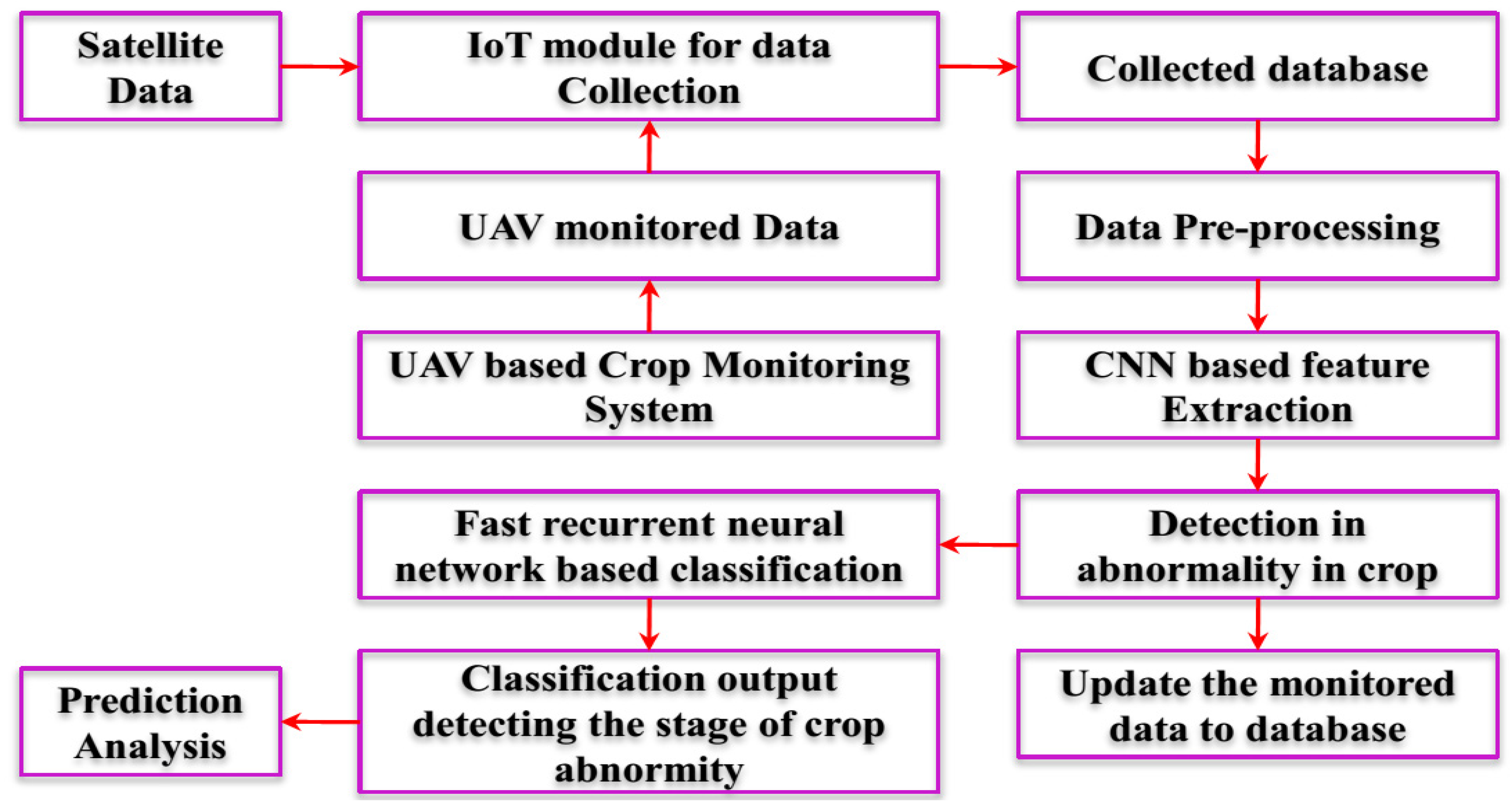
The recent advancements in technology using UAV and Deep Learning approaches have made several impossible things possible. UAV with IoT system help to collect the aerial data with the help of sensors. Geostationary satellites are used to obtain the data and are designed to provide more localized communication services. They typically have an altitude of 35,800 km and include both broadcast and telecommunications satellites in the C-band, Ku-band, and Ka-band frequencies. The useful data can further be used by feeding them to a trained deep learning approach like Artificial Neural Network for prediction. The results are highly helpful for determining an appropriate crop to sow in a particular field. This section presents the UAV design, IoT design, pre-processing phase, feature extraction, and classification of the weed from the original crop, which is considered abnormal data in this study. The proposed Architecture is given in Figure 1.
CNN methods are used for the detection of weeds from crops, mostly because they are the best for image recognition and classification tasks [30]. Unlike other techniques, CNNs are able to identify complex patterns and shapes in data, without having to use “expert knowledge” or manually crafted features. Additionally, CNNs are able to exploit the spatial correlations present in data more effectively, which is especially useful for tasks such as weed detection, as it requires understanding spatial relationships between pixels. Finally, CNNs are fast, powerful and can be used with large datasets, which is important for accurate and precise weed detection. The proposed system is shown in Figure 2.
Initially, the satellite data are pre-processed via resizing, noise removal, and data cleaning, which is then segmented for image enhancement, edge normalization, and smoothening. The segmented image has been pre-trained using CNN for extraction of the feature. Through this process, crop abnormality has been detected. When the abnormality of input data is detected then the data have been classified to predict the stage of crop abnormality. Here, the fast recurrent neural network-based classification has been used. pH and soil nutrient levels are two essential pieces of information provided by electrochemical sensors for precision farming. Specific ions in the soil are found using sensor electrodes to gather data. High-resolution crop data are gathered by drones like the DJI Inspire 2 to spot any problems with the crops and alert growers so they may take prompt action before damage occurs. At the moment, sensors mounted on specifically constructed “sleds” assist in gathering, processing, and mapping soil chemical data. The following section will briefly discuss the extraction of features and data classification.

2.1. CNN-Based Feature Extraction

CNN is used to generate features automatically and combine these with the classifier. Out of all classifiers, the recording of stages that transform appropriate volume into output volume is straightforward in this approach, which is one of the benefits of the CNN classifier [16,17,18,19,20,21,22,23,24]. There are a few distinct layers, and each layer transforms the input into the output using a special function [24,25,26,27,28,29]. This classifier’s disadvantage is that it does not factor in the article’s position and orientation while making predictions. Compared to, say, max pool, both backward and forwards, convolution is a significant leisure operation. Each training step is meant to become significantly longer if indeed the network is large [30,31,32,33,34,35].
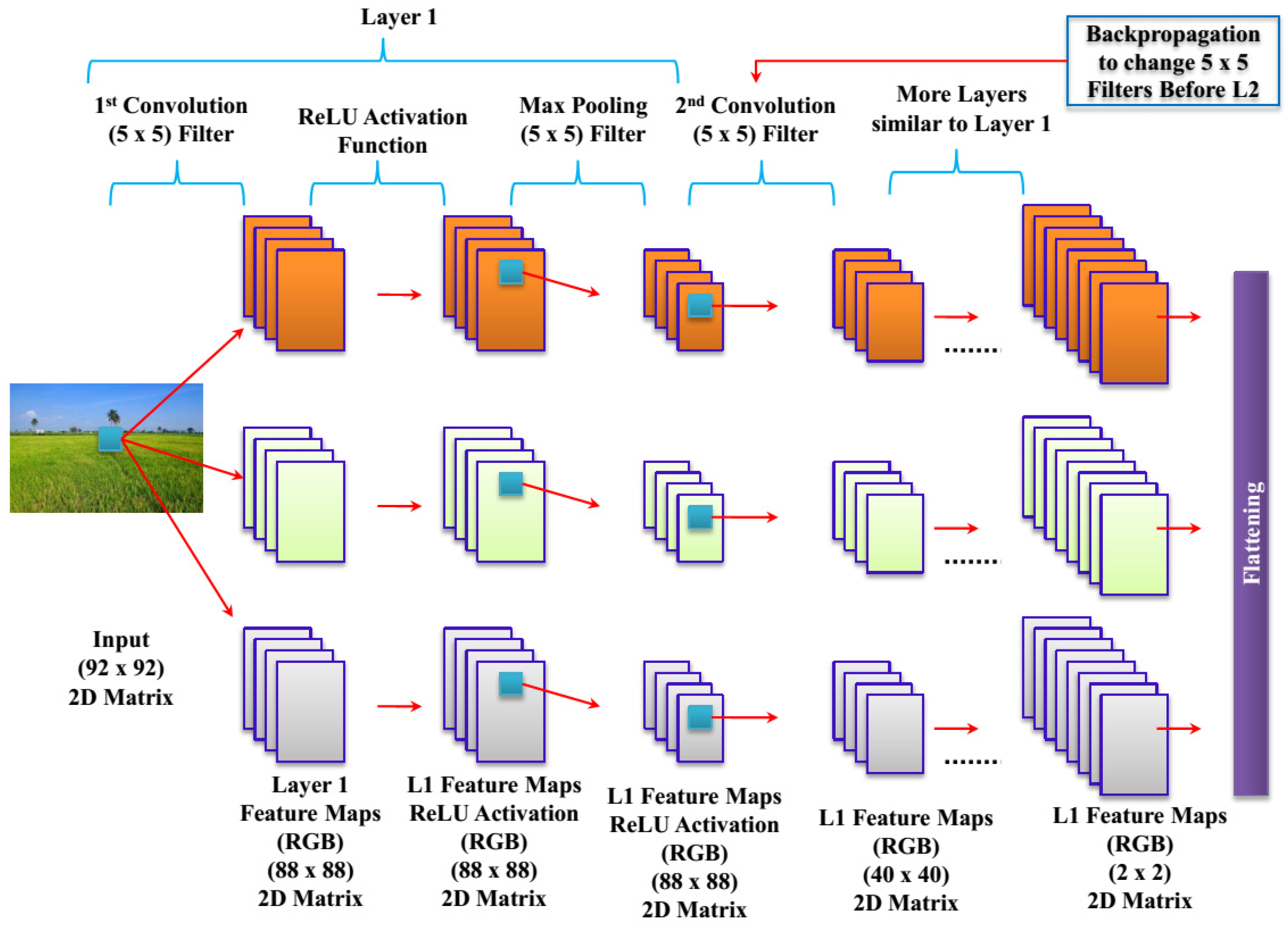
Initially, a Convolutional neural network is employed when the input images are sent to several layers, like convolution, pooling, flattening, and fully connected layers, and a product of CNN is created that categorizes video frame images [34,35,36,37,38,39,40]. After it is established, CNN builds its models from scratch and then uses picture augmentation to improve them. To categorize pictures and assess accuracy for training and testing data, a few of the pre-trained CNNs are employed.
Pool: The pooling layer is referred to as this. In CNN, only maximum pooling is employed, and the pooled kernel size is typically 2 by 2 along a stride of 2.
Fully Connected (FC) layer: The size configuration of this layer’s convolution in CNN is n1 n2, where n1 and n2 are the incoming and outgoing tensors’ respective sizes. N2 is often an integer, whereas N1 is indeed a triplet (7 7 512).
Dropout: The “Drop” layer is used to improve the deep learning technique. In both dropout layers, it puts a small portion of the amount that has been connected to a certain node % networking to 0 and MVGG 16 is set to 0.5.
It is believed that remote sensing provides advantages to some extent over other image-analyzing and machine learning approaches [41,42,43,44,45]. Such methods employ on-ground images successfully to motivate further research works in this area. But few limitations are found with proximal sensing, which makes it difficult to use practically in real-time applications, and increases its nonlinearity [46,47,48,49]. Both of the pooling layers’ convolution layers have the same link code, block size, and stride. In reality, combining two 3 × 3 convolution layers yields one 5 × 5 layer and three 3 × 3 convolution kernels yield one 7 × 7 layer, respectively. A single large convolution kernel performs substantially more slowly than stacking two or three smaller ones. Additionally, the number of parameters has been reduced. Really helpful ReLU layers are those that are added between convolution layers that are too thin.
The object-oriented approach was used to extract useful objects using the multi-resolution segmentation [16] and classification approach [17], where better classification accuracy was obtained compared to the pixel-based approach for spectrum information [18,19,20,21,22,23]. The computational load was heavy while pre-processing and processing data. The high spatial resolution images of UAV produced complex pre-processing and took more time for classifications; thus, it is believed that remote sensing provides advantages to some extent over the other image analyzing and machine learning approaches [23,24,25,26,27,28]. Designing a model that maps StoM with the aid of certain learning data is the main goal. Learning the distribution across labels model, which is denoted as follows, models this as a probabilistic technique.
P ( n ( M , i , w m ) | n ( S , i , w s ) )
where in n (I, i,w) is a rework for an image I that is centered on pixel I and has a size of w * w. In this case, a greater value of w s is better, since it allows for the extraction of more contextual data.
f i s = σ a i s = P ( m i = 1 | s )
where as I and f i respectively represent the total intake once more for the ith output and also the significance of the ith collecting information. The expression for a technical value, (x), is
σ x = 1 1 + e x p ( x )
CNN is used in conjunction with both of the pooling layers’ convolution layers, which have the same link code, block size, and stride. It is given as:
f i l s = e x p ( a i l ( S ) Z = P ( m i = l | s )
where f i l s is the prediction probability in which the pixels mapped to label j.
The structure of CNN is given in Figure 3 below.
The benefits of the suggested technique are enumerated as follows:
  • First, CNN could be able to process enormous amounts of labeled data from different domains.
  • Second, it runs quicker when parallelized with graphics processing units (GPU). As a result, this is also expanded to include additional pixels.
  • Training data are simulated by reducing kernel size through the computational learning procedure of the suggested technique. Optimization becomes challenging, since there are so many training patches. A binary classifier with minimal changes can be used for this. A few of the hyperparameters have been slightly changed. The hyperparameters have been analyzed using sensitivity so that they may be tweaked more precisely.

2.2. Fast Recurrent Neural Networks (FRNN) Based Classification

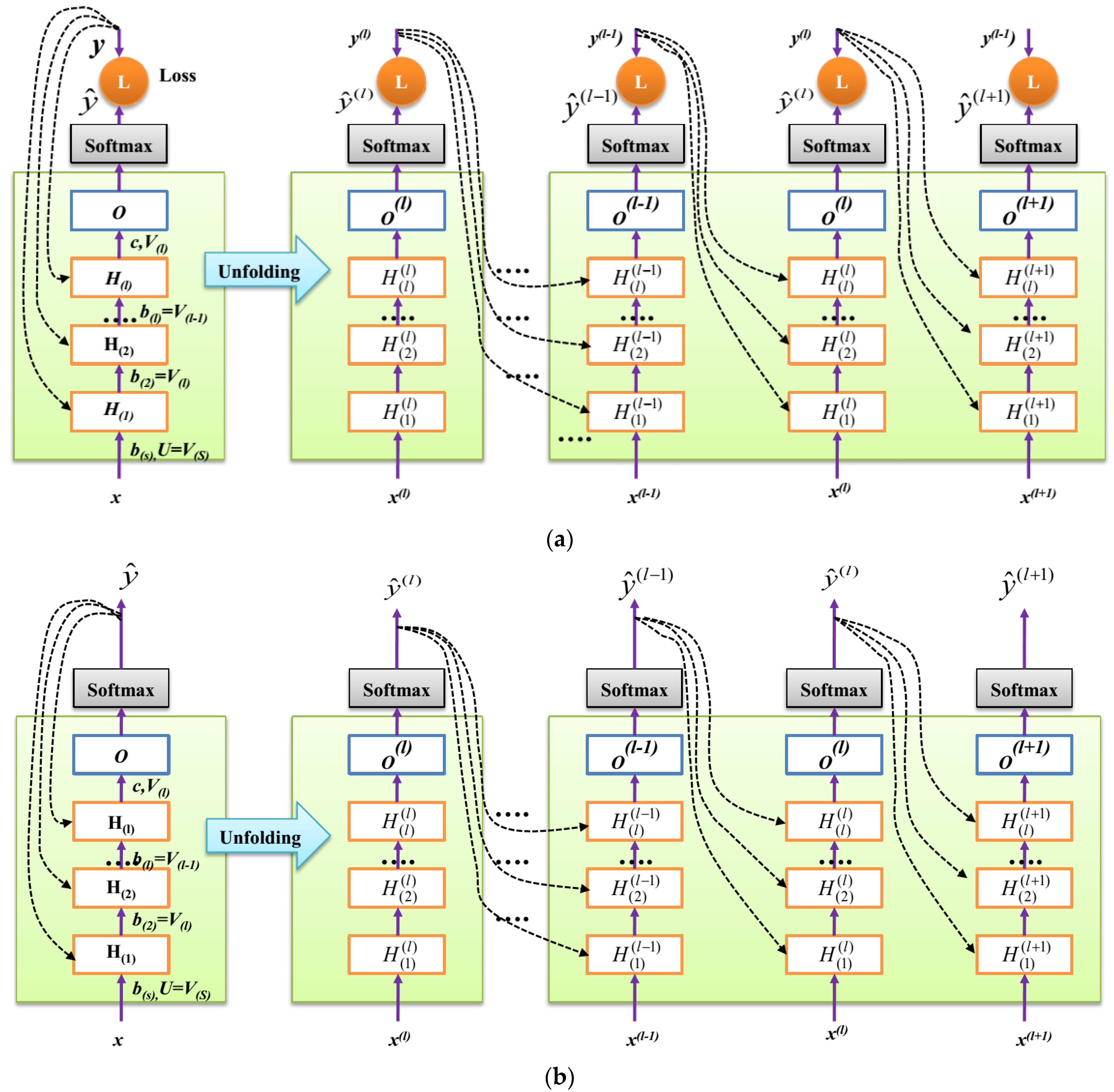
The recurrent architecture along with its unfolded graph of computation for the proposed FRNN is illustrated in Figure 4 for the training and testing phases. As shown in Figure 4a, for each step t, x(t) is provided as follows, and thus x(t) R D, in which D is the component of the functionality input, initiation of the hidden layer is represented by H(t) (k), in which H(t) (k) R ek, signifies the hidden layers number for the layer k, in which 1 k l), and O(t), symbolizes the un-normalized (t).
The m—dimensional U [e1D] is used to parameterize connections between both the hidden and output layer, the graded matrix V(k) [ek + 1ek] is used to characterize interconnection between both the hidden and hidden forwards layers, and the weighted matrix V(k) [Sek] is used to characterize interconnection between both the hidden and output layers. It is interesting that, depending on the distribution of varying input data, ek (1 k l) might change; this refers to k with both the data streams while training. Additionally, in the P-FRNN structure illustrated in Figure 4, recurring connections here between hidden layers are explicitly maintained via hyperplane activity and are indicated as dot-filled arrows.
Additionally, P-FRNN does not maintain an external set of weights for the efficient system between the hidden layer and the output.
As a result, especially for deep networks, the set of indicators in the system is drastically decreased. Further, exploiting the relationship between hidden and outputs is advantageous for the system in terms of learning from exact inputs with older date stamps, and even facilitates greater parallelization when training.
In this section, (k) ∈ bias at level k is R, ek with respect to the (k − 1)th feature plane in which dimension is added. In general, it is noteworthy that the outcome of the previous age stamp implicitly impacts each learning algorithm—with this stimulation being hyperplane dependent—without implicating either parameter or external strength training. Particularly, during testing, the anticipated output, denoted by yb(t1), substitutes for the output, denoted by y(t1), which was acquired as a real forward-propagation estimate Hyperplane in P-FRNN that is implemented by activating the concealed layer. This is used to produce this:
H k = e η d k i t m a x d k i t
where I ranges from 1. Both of the pooling layers’ convolution layers have the same link code, block size, and stride. At the kth hidden layer, di(t) (k) is (t − 1)th data and ith feature in the hyperplane distance as:
d ( 1 ) i ( t ) = y t 1 1 S ( b 1 i + U i x ( t ) ) 1 + j = 1 D U i j 2
where k is 1, the 1-norm of y is |y|1, the dimension of output is S, and R e1 equals the bias at level 1 that belongs to b(1), with respect to the additional aspect of the feature plane. Likewise, for 1 < k ≤ l,
d ( 1 ) i ( t ) = y t 1 1 S . ( b k i + V ( k 1 ) i ) H ( k 1 ) ( t ) 1 + j = 1 e k 1 V ( k 1 ) i j 2
The output that is non-normalized at example t is calculated after obtaining the hidden layer installations, as shown in Figure 4b using:
O t = c + V ( K ) H k ( t )
Therefore, c is the hidden and output bias, denoted by R S, whereas k is equal to l. In order to obtain the expected output yb(t), the non-normalized logarithmic probability is generated and is again normalized using the softmax activation function, and this is provided by:
y ( t ) ^ = s o f t m a x O t
L y , y ^ = i y i . log y ^
L stands for loss which is produced in various ways, and measured outputs at the given time are represented by the y band y.

2.3. Gradient Computing with Back-Propagation

The Back-Propagation SGD technique for the graph that is unwrapped for computation is all that is required in P-FRNN to compute gradients. Additionally, the repeated relationship between the hidden layer and the output is unclear. The traditional back-propagation through-time technique used on RNN for the efficient system between hidden units exhibits problems about exploding/vanishing trend lines, but this approach uses back-propagation to isolate each time stamp, which significantly reduces the calculation time or even defeats those issues. As a result, the following P-FRNN gradient calculation for each timestamp is presented: recursive calculation initially starts with L/L(t) = 1 and is expanded for both the output units and for hidden units, which are as follows:
L O i ( t ) = O t L i = y ^ t y i t
H ( k ) ( t ) L = V k T O t L
H ( k ) ( t ) L = H k + 1 t H k t H k + 1 t L = V k T η M . H k + 1 t . H k + 1 t L
where ‘◦’ indicates the product element-wise and M is the maximum distance beginning on the sample towards the feature plane (k + 1). Both of the pooling layers’ convolution layers have the same link code, block size, and stride. In reality, combining two 3 × 3 convolution layers yields one 5 × 5 layer and three 3 × 3 convolution kernels yield one 7 × 7 layer, respectively. A single large convolution kernel performs substantially more slowly than stacking two or three smaller ones. Additionally, the number of parameters has been reduced. Really helpful ReLU layers are those that are added between convolution layers that are too thin.
For bias parameters, the gradient computation is:
c L = O t c T O t L = O t L
b ( k ) L = ( H k + 1 i H k i ) T H k t L = η M . H k + 1 i · H k t L
where in 1 ≤ k ≤ l. M is indeed the ideal separation between the features on showcase plane k and the samples on a particular occurrence.
The gradients calculation for the weighting component is:
( k ) L = i L O i t V O i t = O i L
If k is assigned as l, then
v ( k ) L = i L H k + 1 i t v k i H k + 1 i t = ( η M . H k + 1 t ) · H k + 1 t L H k t T
if 1 ≤ k < l.
At this point, ∇V(t) represents the weight donation to the gradient at instance t.

2.4. Hidden Layer Online Adaptation

The formalization of the P-self-evolution FRNN’s plan, which would be predicated upon that network significance (NS) model, is presented in this section. Essentially, NS is the theoretically expressed derived form of the mean square error (MSE) for prediction, which is expressed as follows:
N S = V a r O + B i a s ( O ) 2
by directly examining the potential for overfitting or underfitting conditions, where (k) ∈ bias at level k is R ek with respect to the (k − 1)th feature plane in which dimension is added. In general, it is noteworthy that the outcome of the previous age stamp implicitly impacts each learning algorithm with this hyperplane-based stimulation, without implicating either parameter or the external strength training. In addition, by default, they view learning using the instructor forcing strategy whilst also training. In particular, during testing, the anticipated output, denoted by yb(t1), substitutes the output, denoted by y(t1), which was acquired as real. Additionally, NS can determine the model’s accuracy throughout the whole data domain for given data distribution. Large NS values indicate either a large dimensionality or a high bias issue. The former shows that the model is underfitting, whereas the former shows that the model is overfitting. The bias-variance in P-FRNN is calculated as follows:
N S = E O 2 E O 2 + E O y 2
In the above equation, E[O] indicates the output of non-normalized expectation. In some instances, t, the E[O] for P-FRNN is recurrently computed as shown below.
E O = c + V · H p H d H = c + V . E H
where
E H = e d max d p ( d ) d d = e ( E ( d ) m a x ( E ( d ) ) )
Now,
E d = ( E d 1 , E d 2 , E d 3 , . E d e k 1 )
where
E d i k = 1 = y 1 b 1 i + U i . x 1 + j = 1 D U i j p x d x
Most of the existing works consider the data normally distributed, and thus p(x) is assumed to be as follows:
N x μ = 1 ( 2 π ) D / 2 1 | x | 1 / 2 { 1 / 2 x μ T x 1 ( x μ ) }
x stands for the vector with dimension D. However, the data streams do not adhere to a particular density strategy and instead represent a combination of distributions. By presuming this rigid normality assumption, p(x) is defined utilizing the Gaussian mixture modeling asp(x) = (i = 1) to release this innovative P-FRNN. ^K[N(x|μi,∑x i)] K stands for the available components, and I is the mixing coefficient where 0 I 1 and _(i = 1) k I = 1. In this case, the class number, K = S, is taken into consideration. After determining the values of the I variance, and mean parameters, the expectation maximization (EM) technique was used to modify each sample individually. So, it is stated as
E | d i | k = 1 = 1 S m = 1 S | y | 1 ( b i + U i · μ m ) 1 + j = 1 D U i j
where µ ≡ [µ1, µ2, · · ·, µS], and µ > m(m = 1,···S) ∈ R D. Conversely, when the level of the hidden layer k > 1:
E d i k > 1 = y 1 b k i + V k 1 i . H k 1 1 + j = 1 D V k 1 i j p H d H = y 1 b k i + V k 1 i . E H k 1 1 + j = 1 D V k 1 i j = | y | 1 b k i + V k 1 i . e E ( d k 1 ) m a x ( k ( d ) ) 1 + j = 1 D V k 1 i j
Following the computation of NS, it is engaged in altering the structural configuration of the hidden layer in the P-FRNN, as follows: The strategy of growing hidden units: This strategy failed to address the growing issue of prejudice. By increasing the complexity of the structural network or by including multiple hidden units in the hidden layer, the higher bias value denoting an equivalent circumstance is resolved. When the following condition is met, these units are added:
μ B i a s t + σ B i a s t μ B i a s m i n + π σ B i a s m i n
where σ B i a s t , μ B i a s t are the SD and mean where b(k) ∈ bias at level k is R ek in respect to the (k − 1)th feature plane in which dimension is added. In general, it is noteworthy that the outcome of the previous age stamp implicitly impacts each learning algorithm with this hyperplane-based stimulation, without implicating either parameter or external strength training. In addition, by default, learning is achieved using the instructor forcing strategy whilst training. Particularly, during testing, the anticipated output, denoted by yb(t1), substitutes the output, denoted by y(t1), which was acquired as real. The parameters b and V are then randomly selected from the range [−1,1] once the hidden node has been added as a new node. However, as the model does not always converge to the range [−1, 1], parameters may potentially be chosen using an adaptive scope selection strategy.
Technique for removing Hidden units: This approach aims to deal with high variance issues that point to overfitting conditions. This problem may be resolved by either simplifying the network layout or by lowering the number of hidden units in the hidden layer. When the following criterion is met, this situation is recognized:
μ V a r t + σ V a r t μ V a r m i n + 2 π σ V a r min
where σ V a r t , μ V a r t are the SD and mean, respectively, at instance, and σ V a r m i n , μ V a r m i n represents the variance’s SD and least mean, respectively, at case t. (k) ∈ bias at level k is R ek with respect to the (k − 1)th feature plane in which dimension is added. In general, it is noteworthy that the outcome of the previous age stamp implicitly impacts each learning algorithm with this hyperplane-based stimulation, without implicating either parameter or external strength training. In addition, by default, the view learning uses the instructor forcing strategy whilst also training. In particular, during testing, the anticipated output, denoted by yb(t1), substitutes the output, denoted by y(t1), which was acquired as real
H S i = lim T i = 1 T H l i ( t ) T
P r u n i n g min i = 1 . e 1 H S i
Inputs are the data obtained from sensors, like temperature, humidity, and moisture sensors. The number of hidden layers present is directly proportional to the level of accuracy. The output will be the decision of the detection of crop abnormality, determining whether it is suitable to grow in that area in the present and future climatic conditions.

3. Experimental Results and Discussion

3.1. Parameter Settings

The experiment was conducted using the present weather conditions as the input values, namely values of temperature, humidity, rain, and moisture sensors. To obtain the results, around 32 truth frames are taken into account. For every frame, the percentage of soil, crop and weed pixels was calculated approximately and then compared with the ones produced by the proposed model. The simulation results are represented below in Figure 4.
The experiment was conducted using the present weather conditions as the input values, namely values of temperature, humidity, rain, and moisture sensors from Table 1. To obtain the results, around 32 truth frames were taken into account. For every frame, the percentage of soil, crop and weed pixels was calculated approximately and then compared with the ones produced by the proposed model. These introduced several solutions for dealing with highly complex segmentation and classification process. The few advantages of UAVs are flying at a lower altitude, being small in size, being lightweight, having high resolution, and their portability. Machine learning approaches with UAVs have attained more scope in scientific areas. Previous research was conducted in the same area using Faster RCNN, SVM and ANN. The result was obtained in terms of accuracy: 87%, 78%, and 83%, respectively. Similarly, the previous study included very limited and similar datasets and obtained some variations in the previous results, whereas our current research study focuses on UAVs and implementing a machine-learning approach and produces the results in terms of accuracy, precision, specificity, and mean error and produced the best result compared to the existing models.
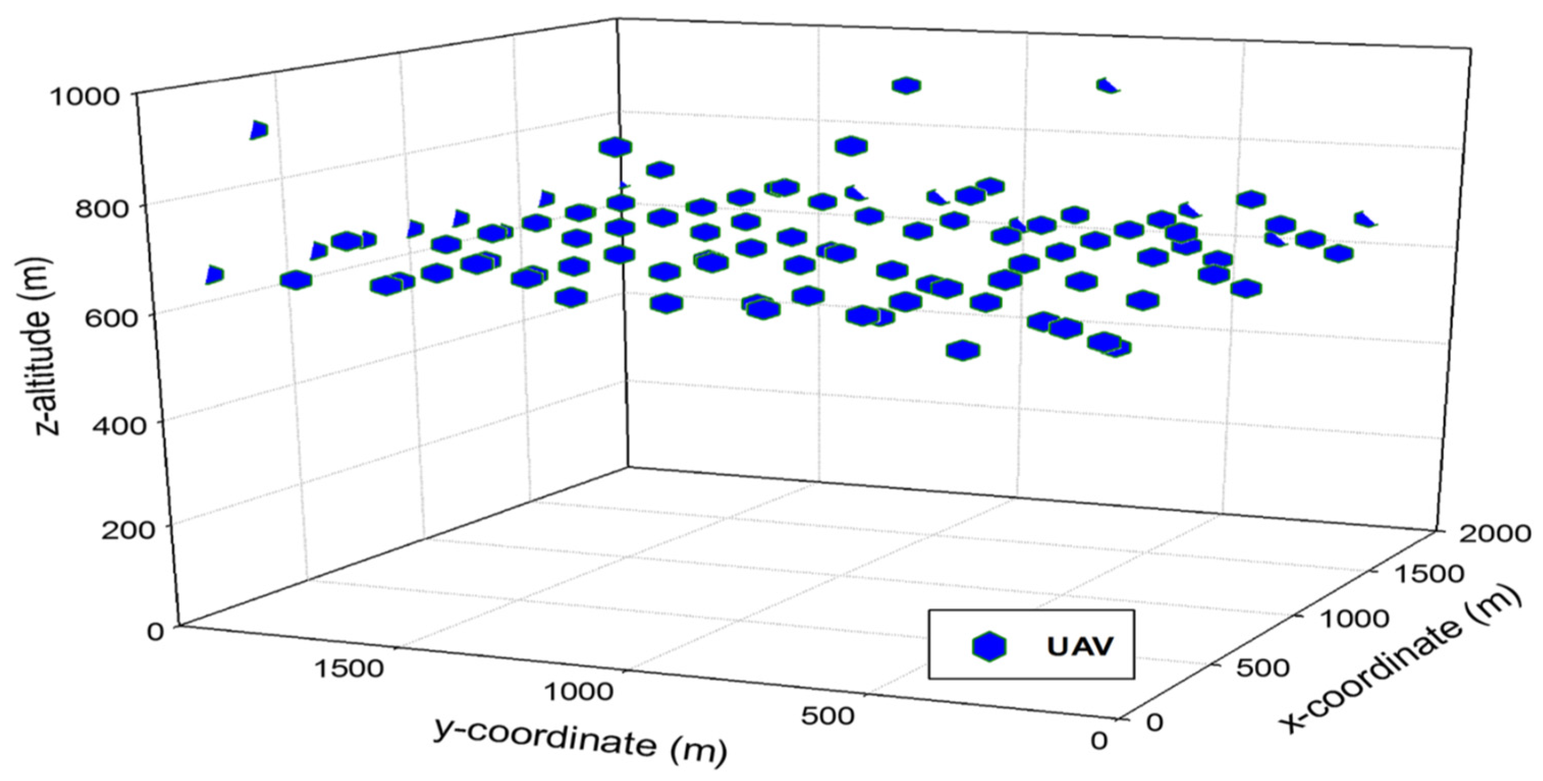
About 100 UAVs were selected because, as can be seen in the writing about UAV correspondence systems, this number is seen as a standard for UAV networks. For all V2V interchanges and for transmitting direct impressions, we set a break term of 1000 s, as this time period is typically used in writing about helpful UAVs, as shown in Figure 5. A representation of the parameters and ranges can be found in Table 1.

3.2. Performance Analysis

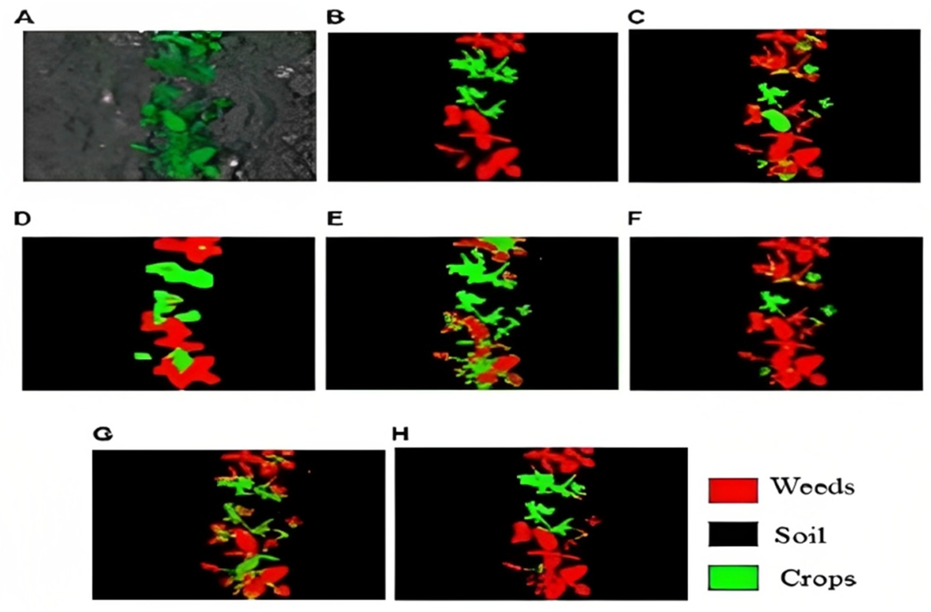
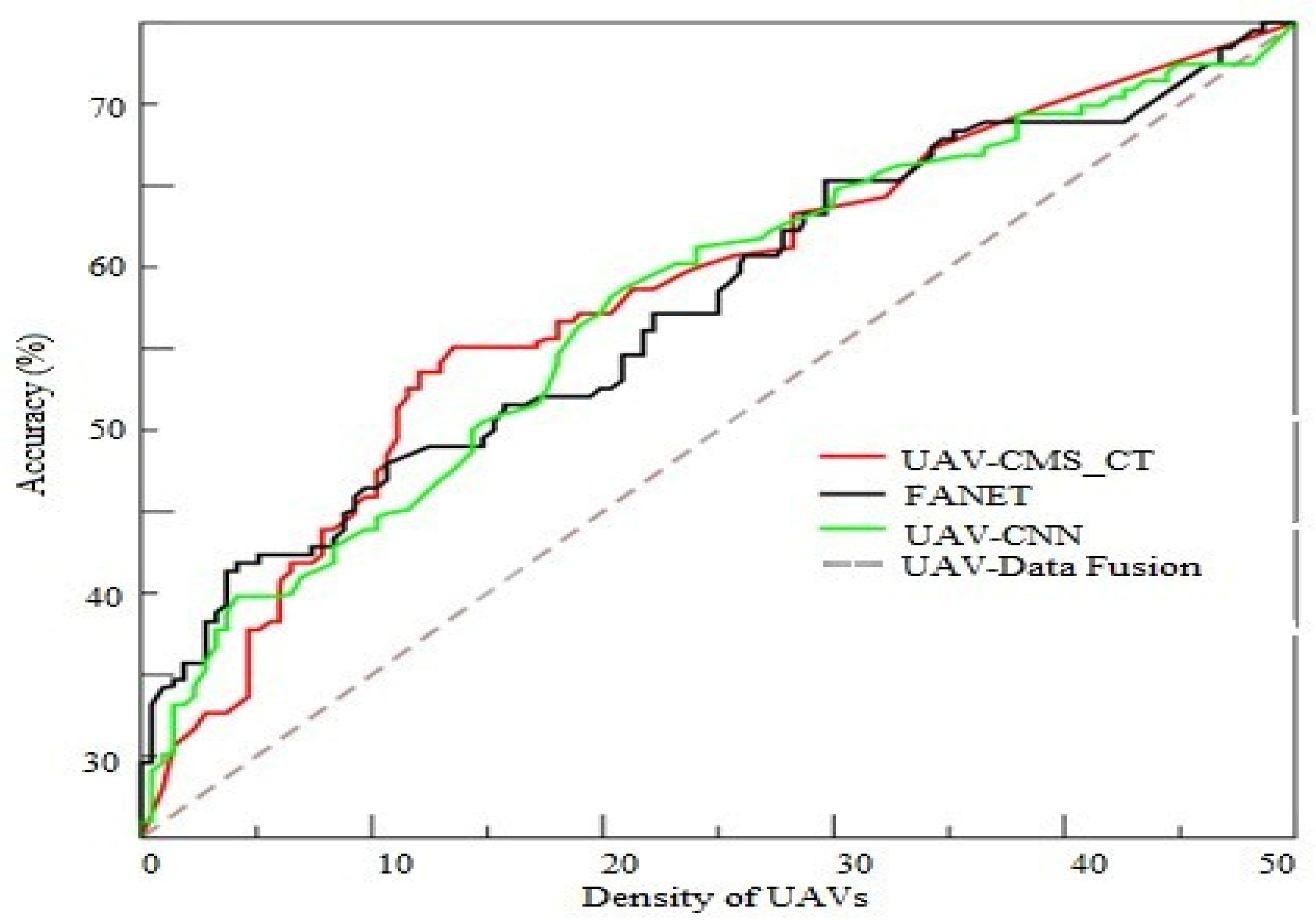
Figure 6 and Figure 7 below represent the weed prediction process of the proposed UAV_ data fusion model with the existing techniques, and the respective qualitative result analysis part has been shown. Figure 7 represents the sugarcane weed prediction and the result analysis of the proposed and existing system is shown. The color shown in both figures represents the crop and weed images taken from the aerial view. The green color represents the crop and the red color represents the weed from the field, which was taken from the UAV aerial images. In the other section, Figure 8 shows the accuracy, precision, specificity, and mean average error comparison for the proposed and existing techniques. The experiment was conducted by giving the present weather conditions as the input values, namely values of temperature, humidity, rain, and moisture sensors. To obtain the results, around 32 truth frames were taken into account. For every frame, the percentage of soil, crop and weed pixels was calculated approximately and then compared with the ones produced by the proposed model.
Figure 8 provides the recent works conducted for weed prediction using computer vision techniques such as UAV-CMS_CT, FANET, UAV-CNN, as well as UAV-data fusion, in which the images are augmented by adding color channels and then trained. The results of the proposed method show a significant improvement in accuracy over the traditional methods. This also indicates that the proposed method can be used for different crop types and different weed species. This experimental analysis provides a detailed analysis of the factors of the proposed model of UAV-data fusion that lead to increased accuracy (93%) compared to the existing techniques UAV-CMS_CT (84%). FANET (87%) and UAV-CNN (91%).
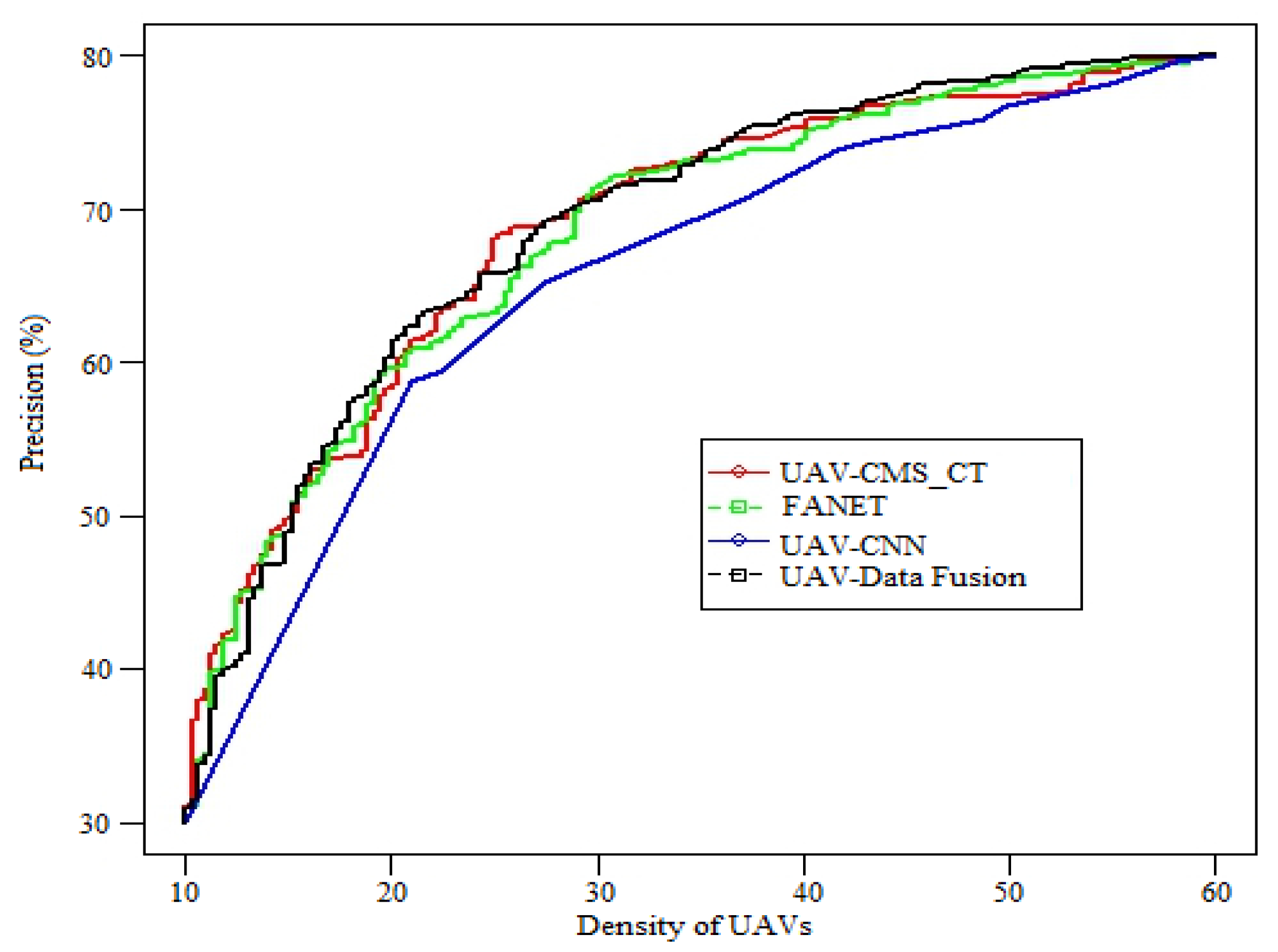
The comparative graphical performance used to determine the precision rate was carried out for various methods, namely the UAV-CMS_CT, FANET, UAV-CNN, as well as UAV-data fusion in Figure 9. A graphical analysis was performed to determine the precision and density of UAV. The experiment was carried out and based on the analysis, the results demonstrate that the proposed approach attained a high precision rate compared with the other existing techniques, as mentioned in Figure 10.
Soil moisture is an important factor in weed detection using UAV-IoT (unmanned aerial vehicle–internet of things). To detect the presence of weeds, UAV-IoT equipped with airborne sensors can measure the soil moisture content near the surface. The soil moisture data collected by the airborne sensors can then be compared with a mapped threshold weed moisture value. If the measured soil moisture content is higher than the mapped threshold value, then it is likely that weeds are present. These data can be used to inform decision-making in weed management initiatives. Additionally, the use of UAV-IoT sensors combined with other variables (e.g., temperature, pH, fertility, etc.) can help enhance weed detection accuracy. Soil moisture is typically calculated using a combination of several methods, including the manual measurements of soil’s water content, soil probes, and soil moisture sensors. Soil probes use both humidity frequency domain reflectometry (H-FDR) and time domain reflectometry (TDR) to measure the dielectric constant of soil, which can then be converted to moisture content.
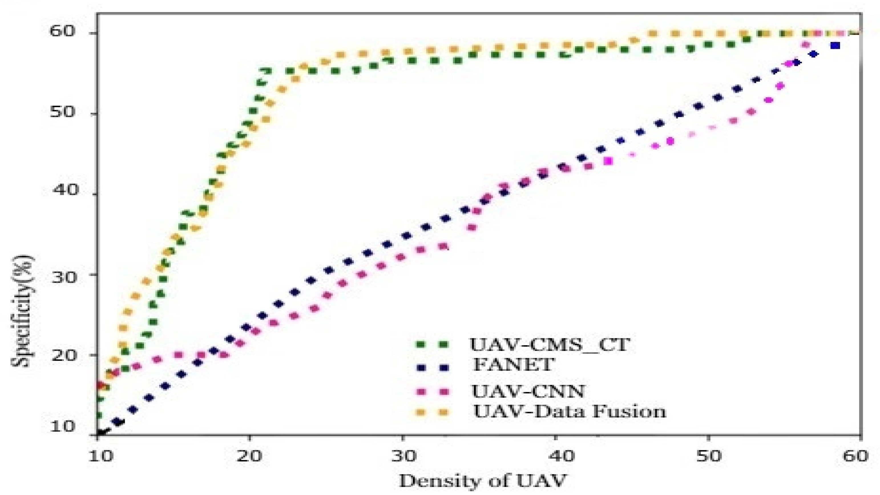
Table 2 also displays the data collected during the initial iterations experiment on this phenomenon, involving the use of sugarcane, potato, and tomato plants. Photosynthesis is a vital process whereby plants generate their own food and energy using light, carbon dioxide, and water. To help achieve this, the stem aids in transporting water and minerals from the roots to the leaves and the products from the leaves to other parts of the plant, such as the roots. Experiments showed that increased soil moisture, meaning higher water content, had a correlation with larger stem diameters. In Figure 11, the comparative analysis is carried out for various methods, namely UAV-CMS_CT, FANET, UAV-CNN, and UAV-data fusion, to determine the specificity rate. The graph plots the accuracy and density of the UAV. The experiment was carried out, and based on the analysis, the results demonstrated that the proposed approach attained a high specificity rate compared with the other existing techniques. Figure 8 shows the mean average error (MAE) value of various methods, namely UAV-CMS_CT, FANET, UAV-CNN, and UAV-data fusion. The proposed method achieved the best MAE value compared to other methods, whereas the other techniques achieved a higher mean absolute error rate compared with other techniques.

4. Conclusions

Agriculture, in the future, may employ sophisticated IoT approaches like temperature and moisture sensors, self-driving agricultural machines, aerial images as well as UAVs, hyper-spectral and multi-spectral imaging devices, as well as positioning technologies, such as GPS. This will depend on the type of sensors being used. This research includes weed sensors used to collect the data from the field and the climate conditions to be measured using thermometers, infrared sensors, and microwave radiometers. Numerous data collected using these technologies are combined with growing technologies of parallel and GPU computing, which have attracted researchers to employ as well as deploy data-driven analysis and deep learning approaches in the agricultural domain. The limitations found using the existing artificial intelligence techniques such as UAV-CNN, UAV_CMS_CT, and FANET are low-resolution images, a lack of high trained data and the need for in-field validation. Here, the IoT-based module is used to collect the data and then CNN-based feature extraction and machine learning-based classification are carried out for the detection of weeds and crops. This system also monitors abnormalities in crops and detects them via feature extraction, and then its level is predicted using an FRNN-based classification technique. The simulation results obtained reveal the optimal accuracy, precision, specificity, and MAE for the proposed design has 0.058 improvement compared with the existing technique. The major benefit of this proposed architecture is the ability of automatic feature extraction achieved by analyzing the time correlation of multiple images, thereby reducing manual feature engineering and modeling crops.

Author Contributions

Conceptualization, Writing—original draft K.V.; Supervision, M.A.A., S.A.-O. and R.S.; Writing—original draft and review and editing, L.A. and T.P.A.; Validation, M.A.A., S.A.-O. and R.S.; propose the new method or methodology, M.A.A., S.A.-O., R.S. and S.S.K.; Formal Analysis, Investigation M.A.A., S.A.-O. and R.S.; Software, L.A. All authors have read and agreed to the published version of the manuscript.

Funding

This work was supported through the Annual Funding track by the Deanship of Scientific Research, Vice Presidency for Graduate Studies and Scientific Research, King Faisal University, Saudi Arabia (Project No. Grant No. 3332) and Princess Nourah bint Abdulrahman University Researchers Supporting Project number (PNURSP2023R136), Princess Nourah bint Abdulrahman University, Riyadh, Saudi Arabia.

Institutional Review Board Statement

Not applicable.

Informed Consent Statement

Not applicable.

Data Availability Statement

Data will be shared for review based on the editorial reviewer’s request.

Conflicts of Interest

The authors declare no conflict of interest.

References

  1. Maimaitijiang, M.; Sagan, V.; Sidike, P.; Daloye, A.M.; Erkbol, H.; Fritschi, F.B. Crop Monitoring Using Satellite/UAV Data Fusion and Machine Learning. Remote Sens. 2020, 12, 1357. [Google Scholar] [CrossRef]
  2. Kwak, G.-H.; Park, N.-W. Impact of texture information on crop classification with machine learning and UAV images. Appl. Sci. 2019, 9, 643. [Google Scholar] [CrossRef] [Green Version]
  3. Vittorio, M. UAV and machine learning based refinement of a satellite-driven vegetation index for precision agricul-ture. Sensors 2020, 20, 2530. [Google Scholar]
  4. Villegas-Ch, W.; García-Ortiz, J.; Urbina-Camacho, I. Framework for a Secure and Sustainable Internet of Medical Things, Requirements, Design Challenges, and Future Trends. Appl. Sci. 2023, 13, 6634. [Google Scholar] [CrossRef]
  5. Su, J.; Coombes, M.; Liu, C.; Zhu, Y.; Song, X.; Fang, S.; Guo, L.; Chen, W.-H. Machine Learning-Based Crop Drought Mapping System by UAV Remote Sensing RGB Imagery. Unmanned Syst. 2020, 8, 71–83. [Google Scholar] [CrossRef]
  6. Zhou, X.; Yang, L.; Wang, W.; Chen, B. UAV Data as an Alternative to Field Sampling to Monitor Vineyards Using Machine Learning Based on UAV/Sentinel-2 Data Fusion. Remote Sens. 2021, 13, 457. [Google Scholar] [CrossRef]
  7. Han, L. Modeling maize above-ground biomass based on machine learning approaches using UAV remote-sensing data. Plant Methods 2019, 15, 10. [Google Scholar] [CrossRef] [Green Version]
  8. Ge, X.; Wang, J.; Ding, J.; Cao, X.; Zhang, Z.; Liu, J.; Li, X. Combining UAV-based hyperspectral imagery and machine learning algorithms for soil moisture content monitoring. PeerJ 2019, 7, e6926. [Google Scholar] [CrossRef]
  9. Ghazal, T.M.; Hasan, M.K.; Abdullah, S.N.; Bakar, K.A.; Al Hamadi, H. Private blockchain-based encryption framework using computational intelligence approach. Egypt. Inform. J. 2022, 23, 69–75. [Google Scholar] [CrossRef]
  10. Guo, Y.; Yin, G.; Sun, H.; Wang, H.; Chen, S.; Senthilnath, J.; Wang, J.; Fu, Y. Scaling Effects on Chlorophyll Content Estimations with RGB Camera Mounted on a UAV Platform Using Machine-Learning Methods. Sensors 2020, 20, 5130. [Google Scholar] [CrossRef]
  11. Eskandari, R.; Mahdianpari, M.; Mohammadimanesh, F.; Salehi, B.; Brisco, B.; Homayouni, S. Meta-Analysis of Unmanned Aerial Vehicle (UAV) Imagery for Agro-Environmental Monitoring Using Machine Learning and Statistical Models. Remote Sens. 2020, 12, 3511. [Google Scholar] [CrossRef]
  12. Zhang, Z.; Al Hamadi, H.; Damiani, E.; Yeun, C.Y.; Taher, F. Explainable artificial intelligence applications in cyber security: State-of-the-art in research. IEEE Access 2022, 10, 93104–93139. [Google Scholar] [CrossRef]
  13. Lottes, P. UAV-based crop and weed classification for smart farming. In Proceedings of the IEEE International Conference on Robotics and Automation (ICRA), Singapore, 29 May–3 June 2017. [Google Scholar]
  14. Ezuma, M.; Erden, F.; Anjinappa, C.K.; Ozdemir, O.; Guvenc, I. Micro-UAV Detection and Classification from RF Fingerprints Using Machine Learning Techniques. In Proceedings of the 2019 IEEE Aerospace Conference, Big Sky, MT, USA, 2–9 March 2019. [Google Scholar] [CrossRef] [Green Version]
  15. Mahmood, S.; Chadhar, M.; Firmin, S. Cybersecurity challenges in blockchain technology: A scoping review. Hum. Behav. Emerg. Technol. 2022, 2022, 7384000. [Google Scholar] [CrossRef]
  16. Zhou, X. Predicting within-field variability in grain yield and protein content of winter wheat using UAV-based mul-tispectral imagery and machine learning approaches. Plant Prod. Sci. 2020, 24, 137–151. [Google Scholar] [CrossRef]
  17. Radoglou-Grammatikis, P.; Sarigiannidis, P.; Lagkas, T.; Moscholios, I. A compilation of UAV applications for precision agriculture. Comput. Netw. 2020, 172, 107148. [Google Scholar] [CrossRef]
  18. Almaiah, M.A.; Al-Zahrani, A.; Almomani, O.; Alhwaitat, A.K. Classification of cyber security threats on mobile devices and ap-plications. In Artificial Intelligence and Blockchain for Future Cybersecurity Applications; Springer International Publishing: Cham, Switzerland, 2021; pp. 107–123. [Google Scholar]
  19. Böhler, J.; Schaepman, M.; Kneubühler, M. Crop classification in a heterogeneous arable landscape using uncalibrated UAV data. Remote Sens. 2018, 10, 1282. [Google Scholar] [CrossRef] [Green Version]
  20. Hall, O.; Dahlin, S.; Marstorp, H.; Archila Bustos, M.; Öborn, I.; Jirström, M. Classification of maize in complex smallholder farming systems using UAV imagery. Drones 2018, 2, 22. [Google Scholar] [CrossRef] [Green Version]
  21. Sharma, B.; Sharma, L.; Lal, C.; Roy, S. Anomaly based network intrusion detection for IoT attacks using deep learning technique. Comput. Electr. Eng. 2023, 107, 108626. [Google Scholar] [CrossRef]
  22. Al Nafea, R.; Almaiah, M.A. Cyber security threats in cloud: Literature review. In Proceedings of the 2021 International Conference on Information Technology (ICIT), Amman, Jordan, 14–15 July 2021; pp. 779–786. [Google Scholar]
  23. Velayudhan, N.K.; Pradeep, P.; Rao, S.N.; Devidas, A.R.; Ramesh, M.V. IoT-enabled water distribution systems-a comparative technological review. IEEE Access 2022, 10, 101042–101070. [Google Scholar] [CrossRef]
  24. Almaiah, M.A.; Hajjej, F.; Ali, A.; Pasha, M.F.; Almomani, O. A Novel hybrid trustworthy decentralized authentication and data preservation model for digital healthcare Iot based CPS. Sensors 2022, 22, 1448. [Google Scholar] [CrossRef]
  25. Nijhawan, R.; Sharma, H.; Sahni, H.; Batra, A. A deep learning hybrid CNN framework approach for vegetation cover mapping using deep features. In Proceedings of the 13th International Conference on SignalImage Technology and Internet-Based Systems, Jaipur, India, 4–7 December 2017; pp. 192–196. [Google Scholar]
  26. Baeta, R.; Nogueira, K.; Menotti, D.; Santos, J.A.D. Learning Deep Features on Multiple Scales for Coffee Crop Recog-nition. In Proceedings of the 30th Conference on Graphics, Patterns and Images, Niteroi, Brazil, 17–20 October 2017; pp. 262–268. [Google Scholar]
  27. Almaiah, M.A.; Ali, A.; Hajjej, F.; Pasha, M.F.; Alohali, M.A. A lightweight hybrid deep learning privacy preserving model for FC-based industrial internet of medical things. Sensors 2022, 22, 2112. [Google Scholar] [CrossRef]
  28. Siam, A.I.; Almaiah, M.A.; Al-Zahrani, A.; Elazm, A.A.; El Banby, G.M.; El-Shafai, W.; El-Samie, F.E.A.; El-Bahnasawy, N.A. Secure health monitoring communication systems based on IoT and cloud computing for medical emergency applications. Comput. Intell. Neurosci. 2021, 2021, 5016525. [Google Scholar] [CrossRef]
  29. Bubukayr, M.A.; Almaiah, M.A. Cybersecurity concerns in smart-phones and applications: A survey. In Proceedings of the 2021 International Conference on Information Technology (ICIT), Amman, Jordan, 14–15 July 2021; pp. 725–731. [Google Scholar]
  30. Alamer, M.; Almaiah, M.A. Cybersecurity in Smart City: A systematic mapping study. In Proceedings of the 2021 International Conference on Information Technology (ICIT), Amman, Jordan, 14–15 July 2021; pp. 719–724. [Google Scholar]
  31. AlMedires, M.; AlMaiah, M. Cybersecurity in Industrial Control System (ICS). In Proceedings of the 2021 International Conference on Information Technology (ICIT), Amman, Jordan, 14–15 July 2021; pp. 640–647. [Google Scholar]
  32. Bah, M.D.; Hafiane, A.; Canal, R. Weeds detection in uav imagery using slic and the hough transform. In Proceedings of the 2017 Seventh International Conference on Image Processing Theory, Tools and Applications (IPTA), Montreal, QC, Canada, 28 November—1 December 2017; pp. 1–6. [Google Scholar]
  33. Kampourakis, V.; Gkioulos, V.; Katsikas, S. A systematic literature review on wireless security testbeds in the cyber-physical realm. Comput. Secur. 2023, 103383. [Google Scholar] [CrossRef]
  34. Almudaires, F.; Almaiah, M. Data an Overview of Cybersecurity Threats on Credit Card Companies and Credit Card Risk Mitigation. In Proceedings of the 2021 International Conference on Information Technology (ICIT), Amman, Jordan, 14–15 July 2021; pp. 732–738. [Google Scholar] [CrossRef]
  35. Suleski, T.; Ahmed, M.; Yang, W.; Wang, E. A review of multi-factor authentication in the Internet of Healthcare Things. Digit. Health 2023, 9, 20552076231177144. [Google Scholar] [CrossRef]
  36. dos Santos Ferreira, A.; Matte Freitas, D.; Gonc¸alves da Silva, G.; Pistori, H.; TheophiloFolhes, M. Weed detection in soybean crops using ConvNets. Comput. Electron. Agric. 2017, 143, 314–324. [Google Scholar] [CrossRef]
  37. Albalawi, A.M.; Almaiah, M.A. Assessing and reviewing of cyber-security threats, attacks, mitigation techniques in IoT envi-ronment. J. Theor. Appl. Inf. Technol. 2022, 100, 2988–3011. [Google Scholar]
  38. Rahnemoonfar, M.; Sheppard, C. Real-time yield estimation based on deep learning. In Proceedings Volume 10218, Autonomous Air and Ground Sensing Systems for Agricultural Optimization and Phenotyping II; SPIE: Bellingham, WA, USA, 2017. [Google Scholar]
  39. Sampathkumar, A.; Murugan, S.; Rastogi, R.; Mishra, M.K.; Malathy, S.; Manikandan, R. Energy Efficient ACPI and JEHDO Mechanism for IoT Device Energy Management in Healthcare. In Internet of Things in Smart Technologies for Sustainable Urban Development; Springer: Berlin/Heidelberg, Germany, 2020; pp. 131–140. [Google Scholar]
  40. Huang, H.; Deng, J.; Lan, Y.; Yang, A.; Zhang, L.; Wen, S.; Zhang, H.; Zhang, Y.; Deng, Y. Detection of helminthosporium leaf blotch disease based on UAV imagery. Appl. Sci. 2019, 9, 558. [Google Scholar] [CrossRef] [Green Version]
  41. Almaiah, M.A.; Hajjej, F.; Lutfi, A.; Al-Khasawneh, A.; Alkhdour, T.; Almomani, O.; Shehab, R. A conceptual framework for deter-mining quality requirements for mobile learning applications using Delphi Method. Electronics 2022, 11, 788. [Google Scholar] [CrossRef]
  42. Latif, G.; Alghazo, J.M.; Maheswar, R.; Sampathkumar, A.; Sountharrajan, S. IoT in the Field of the Future Digital Oil Fields and Smart Wells. In Internet of Things in Smart Technologies for Sustainable Urban Development; Springer: Cham, Switzerland, 2020; pp. 1–17. [Google Scholar]
  43. Wiling, B. Monitoring of Sona Massori Paddy Crop and its Pests Using Image Processing. Int. J. New Pract. Manag. Eng. 2017, 6, 1–6. [Google Scholar] [CrossRef]
  44. Althunibat, A.; Almaiah, M.A.; Altarawneh, F. Examining the factors influencing the mobile learning applications usage in higher education during the COVID-19 pandemic. Electronics 2021, 10, 2676. [Google Scholar] [CrossRef]
  45. Arumugam, S.; Shandilya, S.K.; Bacanin, N. Federated Learning-Based Privacy Preservation with Blockchain Assistance in IoT 5G Heterogeneous Networks. J. Web Eng. 2022, 21, 1323–1346. [Google Scholar] [CrossRef]
  46. Sampathkumar, A.; Tesfayohani, M.; Shandilya, S.K.; Goyal, S.B.; Jamal, S.S.; Shukla, P.K.; Bedi, P.; Albeedan, M. Internet of Medical Things (IoMT) and Reflective Belief Design-Based Big Data Analytics with Convolution Neural Network-Metaheuristic Optimization Procedure (CNN-MOP). Comput. Intell. Neurosci. 2022, 2022, 2898061. [Google Scholar] [CrossRef]
  47. Murugan, S.; Sampathkumar, A.; Raja, S.K.S.; Ramesh, S.; Manikandan, R.; Gupta, D. Autonomous Vehicle Assisted by Heads up Display (HUD) with Augmented Reality Based on Machine Learning Techniques. In Virtual and Augmented Reality for Automobile Industry: Innovation Vision and Applications. Studies in Systems, Decision and Control; Hassanien, A.E., Gupta, D., Khanna, A., Slowik, A., Eds.; Springer: Cham, Switzerland, 2022; pp. 45–64. [Google Scholar] [CrossRef]
  48. Jat, N.C.; Kumar, C. Design Assessment and Simulation of PCA Based Image Difference Detection and Segmen-tation for Satellite Images Using Machine Learning. Int. J. Recent Innov. Trends Comput. Commun. 2022, 10, 1–11. [Google Scholar] [CrossRef]
  49. Vaidhehi, M.; Malathy, C. An unique model for weed and paddy detection using regional convolutional neural networks. Acta Agric. Scand. Sect. B—Soil Plant Sci. 2022, 72, 463–475. [Google Scholar] [CrossRef]
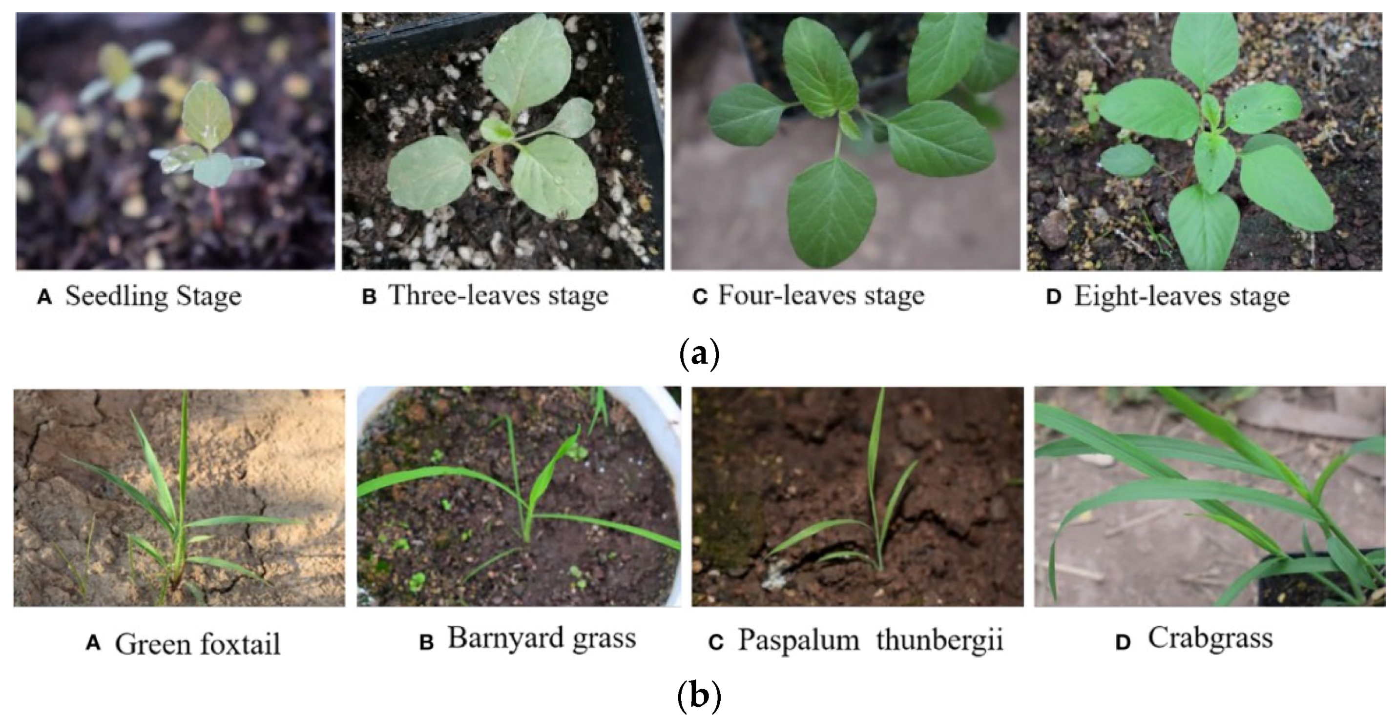
Figure 1. (a) Sample images of crops; (b) sample images of weeds.
Sustainability 15 11242 g001
Figure 2. Proposed Architecture.
Sustainability 15 11242 g002
Figure 3. CNN architecture for feature extraction.
Sustainability 15 11242 g003
Figure 4. Proposed FRNN design (a) Training phase, (b) test phase.
Sustainability 15 11242 g004
Figure 5. Simulation scenario.
Sustainability 15 11242 g005
Figure 6. Qualitative Analysis of Weed is achieved for CWFID dataset. (A) Input Images (B) Groundtruth (C) SegNet (D) UAV-CMS_CT (E) FANET (F) FCN (G) UAV_Data Fusion (H) UAV_CNN.
Sustainability 15 11242 g006
Figure 7. Qualitative Analysis of Weed is achieved for the sugarcane dataset. (A) Input Images (B) Groundtruth (C) SegNet (D) UAV-CMS_CT (E) FANET (F) FCN (G) UAv_Data Fusion (H) UAV_CNN.
Sustainability 15 11242 g007
Figure 8. Comparison of accuracy.
Sustainability 15 11242 g008
Figure 9. Comparison of precision.
Sustainability 15 11242 g009
Figure 10. Comparison of specificity.
Sustainability 15 11242 g010
Figure 11. Comparison of mean average error.
Sustainability 15 11242 g011
Table 1. Representation of parameters and ranges.
ParametersRanges
Pooling layer2 by 2 along a stride of 2
Activation functionReLu
Learning rate0.001
WeightRandom normal distribution
Method of poolingMax pooling function
Table 2. Soil moisture analysis table.
SL.NOSoil Moisture Experimental Analysis
Rainfall (mm)Soil Moisture (%)Temperature (°C)Humidity (%)
1100512478
2200492478
3300492478
4400492478
5500502478
Disclaimer/Publisher’s Note: The statements, opinions and data contained in all publications are solely those of the individual author(s) and contributor(s) and not of MDPI and/or the editor(s). MDPI and/or the editor(s) disclaim responsibility for any injury to people or property resulting from any ideas, methods, instructions or products referred to in the content.