Power-Weighted Prediction of Photovoltaic Power Generation in the Context of Structural Equation Modeling

Abstract

With the popularization of solar energy development and utilization, photovoltaic power generation is widely used in countries around the world and is increasingly becoming an important part of new energy generation. However, it cannot be ignored that changes in solar radiation and meteorological conditions can cause volatility and intermittency in power generation, which, in turn, affects the stability and security of the power grid. Therefore, many studies aim to solve this problem by constructing accurate power prediction models for PV plants. However, most studies focus on adjusting the photovoltaic power station prediction model structure and parameters to achieve a high prediction accuracy. Few studies have examined how the various parameters affect the output of photovoltaic power plants, as well as how significantly and effectively these elements influence the forecast accuracy. In this study, we evaluate the correlations between solar irradiance intensity (GHI), atmospheric density (ρ), cloudiness (CC), wind speed (WS), relative humidity (RH), and ambient temperature (T) and a photovoltaic power station using a Pearson correlation analysis and remove the factors that have little correlation. The direct and indirect effects of the five factors other than wind speed (CC) on the photovoltaic power station are then estimated based on structural equation modeling; the indirect effects are generated by the interaction between the variables and ultimately have an impact on the power of the photovoltaic power station. Particle swarm optimization-based support vector regression (PSO-SVR) and variable weights utilizing the Mahalanobis distance were used to estimate the power of the photovoltaic power station over a short period of time, based on the contribution of the various solar radiation and climatic elements. Experiments were conducted on the basis of the measured data from a distributed photovoltaic power station in Changzhou, Jiangsu province, China. The results demonstrate that the short-term power of a photovoltaic power station is significantly influenced by the global horizontal irradiance (GHI), ambient temperature (T), and atmospheric density (ρ). Furthermore, the results also demonstrate how calculating the relative importance of the various contributing factors can help to improve the accuracy when estimating how powerful a photovoltaic power station will be. The multiple weighted regression model described in this study is demonstrated to be superior to the standard multiple regression model (PSO-SVR). The multiple weighted regression model resulted in a 7.2% increase in R², a 10.7% decrease in the sum of squared error (SSE), a 2.2% decrease in the root mean square error (RMSE), and a 2.06% decrease in the continuous ranked probability score (CRPS).

1. Introduction

Solar energy is an important source of clean energy due to its plentiful supply and lack of pollutants. The use of solar energy on a large scale is essential to reaching the carbon peak and becoming carbon neutral. However, due to the variations in solar radiation and weather, solar power generation varies and is intermittent, which affects the dependability and security of the power grid [1,2,3]. At the same time, meteorological factors change in a short period, resulting in instantaneous or short-term volatility and randomness of photovoltaic power generation [4]. In order to use solar energy more efficiently, it is crucial to accurately predict the photovoltaic output power over a short period of time [5].

Numerous techniques have thus been developed to predict the photovoltaic output power over a short period of time, in accordance with the aforementioned variables, as solar radiation variations and meteorological conditions are significant factors that influence the photovoltaic output power variation [6]. Physical methods [7], statistical prediction methods [8], and integrated prediction methods [9] can all be used to predict the photovoltaic output power. The physical methods are typically based on the photovoltaic power generation principle, and the location of the photovoltaic power station, the installed capacity, the characteristic parameters of the photovoltaic panels, the installation inclination of the photovoltaic modules, and other information are all used to establish a prediction model describing the mapping relationship between the photovoltaic power station and solar irradiance [10]. However, systematic divergence will result if the established prediction model is unreliable and if the underlying data are incorrect or insufficient. Instead of the physical process of photovoltaic power generation, which has modest equipment requirements and a quick forecast time, the statistical prediction approach is typically based on the statistics of historical observation data [11,12]. However, there can be several extreme points of photovoltaic power under non-clear sky situations, because of the wide variation in meteorological elements, which causes forecasting instability. Based on physical methods and statistical prediction methods, the term “combined prediction method” refers to a prediction method that is created by fully combining the characteristics of the data from a photovoltaic power station and meteorological data, as well as by weighting the combinations of the different prediction methods, such as physical methods and statistical methods. The integrated prediction technique includes a significant role for artificial intelligence. There are currently two main combination methods. (1) Weighting of the predictions of the various prediction methods, with the multiple regression model (MRM), genetic algorithms, and artificial neural networks (ANNs) serving as a typical approach, is used to yield the final prediction results. (2) The historical photovoltaic data are decomposed into various sub-sequences, and the multiple sub-sequences are then independently predicted, and then superimposed to obtain the final prediction results. Typically, this is performed using wavelet analysis or empirical mode decomposition (EMD). The non-stationary data are decomposed before an ANN or another method is used to predict the power. The combined forecasting approach can maximize the benefit of each individual forecasting method and increase the precision of photovoltaic power forecasting. As a result, the combined forecasting methods are more frequently utilized when predicting the photovoltaic output power over a short period of time. A multi-channel convolutional neural network model was built by Heo et al. [13] to estimate photovoltaic output power using solar radiation and four additional meteorological parameters, which obtained promising prediction results. The method uses equal weights for the five input parameters to predict the photovoltaic output power, ignoring the variability in the contribution of solar radiation and additional weather elements. In order to study the relationship between the power output and environmental conditions, Luo et al. [14] developed a short-term prediction model based on support vector machine regression and a PSO-RIDGE wave neural network model based on principal component analysis (PCA-SVR). The number of input environmental elements is decreased, but the primary components are extracted by the use of PCA. The ridge wave neural network’s parameters are chosen using particle swarm optimization (PSO). Then, in order to improve the model’s performance, the network structure is optimized using the SVR model. This technique offers a good forecast accuracy, and essentially eliminates the impact of the interference of weather elements. However, this method only selects the elements that have a large impact on the photovoltaic output power and ignores the contribution of the less influential elements in the photovoltaic output power prediction. Pierro et al. [15] created a combined multi-model ensemble (MME) prediction model, which incorporates numerous sub-models and various meteorological elements as the input variables. Finally, a more precise prediction impact was attained by using the weighted combination of the results of the sub-models.

Most of the current research on the use of the combined prediction method to predict the solar output power has concentrated on how to increase the prediction accuracy by changing the model structure or parameters [16,17]. This kind of method can accurately predict the photovoltaic output power based on various methods [18]. However, the above combined prediction methods only achieve an accurate photovoltaic output power prediction from a “data-driven” perspective via the feature selection of input elements, the adjustment of the model structure, and the improvement in the training strategy, while ignoring the effect of different solar radiation and weather elements on the photovoltaic output power prediction under realistic conditions. In addition to negligible minor effects, elements that contribute less to the photovoltaic output power prediction should not be ignored. In view of this, in this paper, based on the contribution of solar radiation and meteorological conditions to the photovoltaic output power, combined with a combined forecasting model, we propose a short-term forecasting method for the photovoltaic output power. On the basis of analyzing the contribution of the different factors to the photovoltaic output power, a combined prediction model with weighted processing of the above factors is used to further improve the prediction performance and prediction effect. A technique used to artificially establish causation through correlation is the structural equation model (SEM) [19]. The complex causal relationship between the solar radiation, weather, and photovoltaic output power can be examined using the SEM. Based on this relationship, a set model can be created using a multiple weighted regression method to accurately predict the short-term photovoltaic output power.

The main contribution of this paper is to propose a short-term weighted prediction method for photovoltaic output power by combining the SEM with the multiple weighted regression technique. First, based on previously reported articles, the SEM was used to examine the effects of six factors, including solar radiation and weather, on the photovoltaic output power. It is worth noting that this influence is the effect of solar radiation and weather elements on photovoltaic output power in a realistic state, rather than feature selection from a “data-driven” perspective only. Then, using the multiple weighted regression approach, a weighted prediction model for the short-term photovoltaic power production was created. This work is aimed at (1) examining how the different variables affect the photovoltaic output power; (2) assessing the effect of the various factors on the photovoltaic output power from multiple aspects, including individual effectiveness and interaction; and (3) building an ensemble model to precisely forecast the short-term photovoltaic output power.

The rest of this paper is structured as follows. The research region and data processing are described in Section 2. Section 3 describes how we built a short-term weighted prediction model for a solar power plant and goes into depth on how to calculate the weights using multiple weighting modules and how to forecast the power using multiple regression modules. The experimental findings are described in Section 4. The validity of the SEM approach is covered in Section 5, along with an assessment of the weights of the photovoltaic power prediction model. The study is outlined and summarized in Section 6.

2. Data Collection and Processing

2.1. Data Collection

Measurement data for the photovoltaic output power (full-field power), global horizontal irradiance (GHI), and ambient temperature (T) of the photovoltaic power station of the Bridgestone Corporation in Changzhou, Jiangsu province, China, were obtained in this study. The power station is situated at an altitude of 10 m, at 31.87° N and 119.98° E, in Xinbei District, Changzhou City, Jiangsu province, China. The project capacity is 3MW. The average value of the total horizontal annual radiant irradiation in the area in the first half of 2018 is 1110.67 kWh/m². The meteorological circumstances have a significant impact on the solar energy resources in this area. The environment for solar power production is complicated and unstable, and the photovoltaic power plants exhibit substantial power fluctuation. Relative humidity (RH), wind speed (WS), cloud cover (CC), and the atmospheric density (ρ) for Changzhou were the simultaneously measured meteorological parameters. The sun radiation data, which refer to the impact of the global horizontal irradiance (GHI) on the power of a small-scale photovoltaic power station, are the major topic of discussion in this work. In addition to the impact of the solar radiation intensity on the photovoltaic power station power, the weather and the power station surroundings are the other factors that affect the power station power [20]. Clouds can be the most significant and direct meteorological phenomenon affecting the short-term full-field power variations of photovoltaic plants [21]. Other parameters that impact the full-field output of solar power plants include air density, humidity, and ambient temperature [22]. The following six variables were gathered as possible influencing factors in this study: global horizontal irradiance (GHI), atmospheric density (ρ), cloud cover (CC), wind speed (WS), relative humidity (RH), and ambient temperature (T).

2.2. Data Preprocessing

The solar irradiance intensity, air density, and ambient temperature were sampled as 15 min averages of the observations among the six potential components recorded from January to June 2018. The relative humidity (RH) and wind speed (WS) are averaged over one hour to form a sample. The cloud cover is a sample of observed 3 h averages. In order to ensure that the observation data and the full-field power of the photovoltaic power station are sampled at the same time, this paper will transform the above data at 3 h intervals. In the conversion, we select the samples of the global horizontal irradiance (GHI), atmospheric density (ρ), wind speed (WS), relative humidity (RH), and ambient temperature (T) that are closest to the sampling time of the cloud cover (CC) to form a data set. A total of 335 daylight samples with a 3 h interval were obtained after modification from January to June 2018. To evaluate the performance of the prediction model, 80% of the samples were randomly chosen as the training set, 10% were chosen as the validation set, and the rest were used as the test set.

3. Short-Cycle Weighted Prediction Model for a Photovoltaic Power Station

3.1. Construction of the Structural Equation Model

3.1.1. Structural Equation Model

A multivariate statistical technique called the structural equation model (SEM) was used to clarify the causal connection between the variables [23]. Different from the usual multivariate statistical method, which enables the measurement of variables with errors, the SEM employs a path graph model and makes it possible to analyze the relationship between the variables. Researchers in the field of ecology [24,25], solar energy [26], and those in other fields have also seen the widespread application of the SEM. The Changzhou photovoltaic power plant in this work is subject to the complicated combined influence of solar radiation, weather conditions, and other elements. It is important to take into account both the direct and indirect effects that the various parameters have on the power of solar power plants, in addition to the direct effects of such elements. Unlike correlation analysis, with which it is challenging to characterize the complex coupling relationship between variables, structural equation modeling is not constrained by the strict assumptions of path analysis and can analyze both the structural relationship between the potential variables and the measurement error. The basic task of the SEM analysis is to simultaneously estimate all of the model’s parameters using the maximum likelihood approach, and to evaluate the model’s overall fit by comparing the theoretical model covariance to the measured covariance. The path coefficients of the path graph model can be obtained via the SEM by computing the covariance matrix between the solar radiation, weather, and photovoltaic power. The method through which the different factors have an impact on the photovoltaic power is then quantitatively described. The relationship between the various influencing factors can be processed through the analysis of the factors affecting the photovoltaic power station, and the contribution of the various influencing factors to the power of the photovoltaic power station can be represented by the path coefficients obtained from the model results. This can then be used as the basis for determining the weights of the short-term weighted prediction model for the photovoltaic power station. The latent variables and the observed variables are the two categories of variables in an SEM. The latent variables are those factor variables that cannot be directly observed and characterized, whereas the observed variables are those that can be directly observed and measured. The potential factors affecting the power of a solar power station, which are collected in Section 2.1 of this article, can be directly observed and characterized. Therefore, in this study, to examine the interaction between the six aforementioned elements and the power of a solar power station, the SEM solely employs the observed variables as the model inputs.

3.1.2. Structural Equation Model Construction Method

Figure 1 depicts the precise procedure for building the SEM. The hypothesis that the solar irradiation intensity and meteorological factors interact with one another and ultimately have an impact on the power of the photovoltaic power station is first put forward. Secondly, the framework of the SEM is established in accordance with the aforementioned hypothesis, and the data are gathered. The model parameters and the model fitting condition are then evaluated. If the model fitting condition is not good, the number of model parameters needs to be readjusted. Finally, the model results are combined with the proposed hypothesis for analysis [19]. In order to establish the fair weight for each influencing component and create a more accurate prediction model, the SEM is utilized to examine the complete effect of the numerous aspects on the solar power station.

3.2. Construction of the Short-Term Weighted Prediction Model for a Photovoltaic Power Station

It is challenging for the current general models to correctly predict the power of a photovoltaic power plant because of the complexity and nonlinearity of photovoltaic power variations. Therefore, a weighted short-cycle prediction model for photovoltaic power plants is suggested based on the efficiency of the various components mentioned above. As shown in Figure 2, the model is composed of two parts; (1) the weight calculation module, which is also known as the multiple weighting module, is used to calculate a fair weight for each influencing element, and (2) the multivariate prediction module is used to perform the weighted regression of the different influencing factors.

3.2.1. Multivariate Weighting Module

The weight calculation module takes into account the direct and indirect contribution degrees of each element to the solar power station and calculates the fair weight for each influencing factor on the basis of route analysis and cluster analysis of the SEM. The Mahalanobis distance, which is independent of the measurement scale, is not impacted by the dimension between the coordinates. Furthermore, the interference of the correlation between the variables can be disregarded because of the wide disparity in the value range between the input variables and the complicated correlation between the variables. As a result, the module bases its weight calculation on the Mahalanobis distance between each factor and the power of the solar power station [27]. In order to eliminate the necessity for an independent and homogeneous distribution, the Mahalanobis distance creates a covariance matrix between the variables based on the Euclidean distance. The Mahalanobis distance is preferable for calculating the power weight of a solar power plant. The Mahalanobis distance is calculated as shown in Equation (1). ${\displaystyle {\sum }_{}^{-1}}$ is the SEM’s calculation of the covariance matrix between the variables, as indicated in Equation (2), where y is the solar power plant’s output, $x_n$ represents the factors influencing that output, Var is the variable’s variance, and Cov is the covariance across the variables. According to the covariance matrix of the SEM, the module calculates the Mahalanobis distance between each influencing factor and the power of the solar power station and inserts these values as weights into the multiple regression module.

$$D_M\left(x,y\right)=\sqrt{{(x-y)}^T{\sum }_{}^{-1}(x-y)}$$

(1)

$$\sum =\left[\begin{array}{ccc}var\left(y\right)& & \\ cov(x_1,y)& var\left(x_1\right)& \\ cov(x_2,y)& cov(x_2,x_1)& var\left(x_2\right)\\ cov(x_3,y)& cov(x_3,x_1)& cov(x_3,x_2)& \ddots & & \\ ⋮& ⋮& ⋮& & var\left(x_{n-1}\right)& \\ cov(x_n,y)& cov(x_n,x_1)& cov(x_n,x_2)& & cov(x_n,x_{n-1})& var\left(x_n\right)\end{array}\right]$$

(2)

3.2.2. Multiple Regression Module

A nonlinear supervised machine learning approach with a high overall performance is the support vector regression (SVR) model. Due to its properties of rapid convergence, minimal parameters, and high reliability, the support vector regression model based on particle swarm optimization (PSO-SVR) is frequently employed in the prediction of solar radiation intensity and photovoltaic power over short periods [14,28,29,30]. Particle swarm optimization (PSO) is used in the multivariate prediction module of the proposed model to optimize the main parameters in the support vector machine model, because of the complicated nonlinear connection between the impact variables chosen in this work and the power of the photovoltaic power. This approach can be used to optimize nonlinear issues and is comparable to genetic algorithms, which employ population fitness data to identify the best solution to a given problem [31,32]. Kennedy and Eberhart [33] were the first to suggest PSO, where each optimization issue solution is treated by the algorithm as a random particle, with a random location and velocity. Each particle records and updates its current location and velocity, as well as both its individual ideal position and the population’s optimal position during the iterative process [34,35]. The iterative formula for updating the velocity and position of each particle in the population is as follows [36,37]. When looking for an optimal solution through an n-dimensional space with m particles forming a population, the position of the i-th particle is denoted as $v_i=(v_1,v_2,\dots ,v_n)$.

$$v_i(t+1)=\omega v_i(t)+c_1{r}_1(p_i(t)-x_i(t))+c_2{r}_2(p_g(t)-x_i(t))$$

(3)

$$x_i(t+1)=x_i(t)+v_i(t+1)$$

(4)

where i = 1,2,3,…n; p_i is the position of an individual extreme point; p_g is the global extreme point position; ω is the initial value of the inertia weight; C₁ and C₂ are the acceleration coefficients; and R₁ and R₂ are random numbers between 0 and 1. For the SVR model, PSO with global convergence can better ensure the rationality of the parameter optimization [36]. The multivariate prediction module applies the aforementioned acceptable weights to the input data and uses the PSO approach to obtain the best model parameters. It is also possible to make SVR models using the PSO technique [38]. The SVR regression function is outlined as follows, in order to obtain quick convergence and prevent the model from being over- or under-fitted:

$$f(x)=\omega x+b$$

(5)

where $\omega$ and b are the SVR model parameters that were learned iteratively. x represents the data from January to June 2018 in Changzhou for the following variables: global horizontal irradiance (GHI), atmospheric density (ρ), cloud cover (CC), relative humidity (RH), and ambient temperature (T).

The inputs for the multiple regression module represented many orders of magnitude of possible variables. For instance, in the training set, the values for temperature varied from −6.8 to 36.7 °C, and those for cloud cover ranges from 0 to 1. As a result, all the input variables were normalized as follows to lie between −1 and 1:

$$X^{\prime }=\frac{X}{\max (X)}$$

(6)

where $X^{\prime }$ is the normalized input variable; $X$ denotes the value of an input variable; and max (X) is the input variable X’s maximum value found in the training set.

4. The Experimental Results

4.1. Multivariate Weighted Results

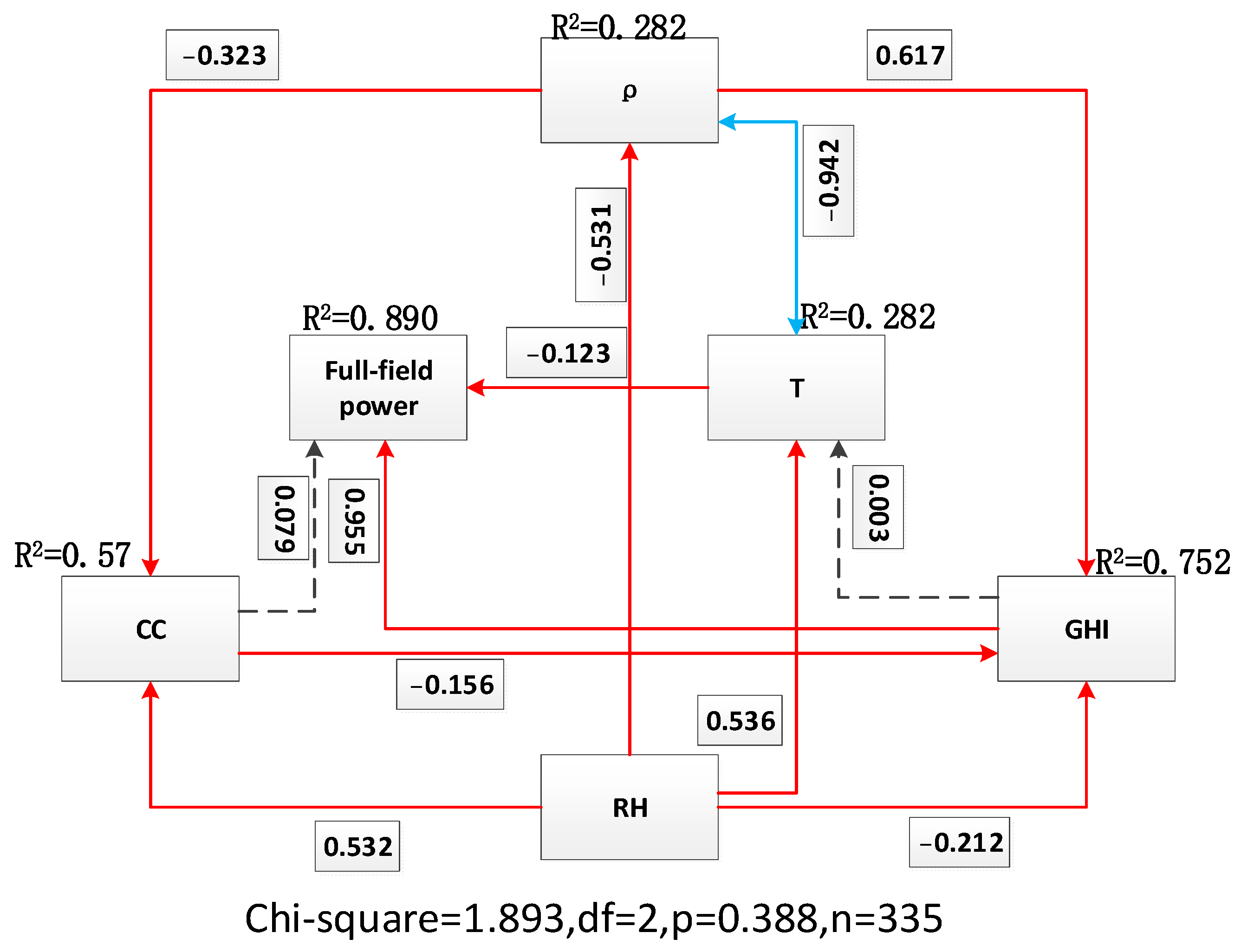
The photovoltaic power can be quickly and correctly forecasted using the multivariate weighted prediction model. Due to the small wind speed (WS) during the study period, its contribution to the photovoltaic power generation is weak [39]. The model’s input parameters are the global horizontal irradiance (GHI), the atmospheric density (ρ), the number of clouds (CC), the relative humidity (RH), and the ambient temperature (T). The path graph model between the solar power plant and the five observed variables is created using the multiple weighting module, as shown in Figure 3. The route diagram shows the observed variables as rectangular boxes, and it shows the causal link between two variables by connecting them with a solid line and a single arrow. A dotted line with an arrow is used to link two variables, showing that they have a minimal impact on one another. A solid line with a double arrow is used to connect two variables, demonstrating the correlation between them. The model was fitted using 335 groups of data in total. Following the fitting, the model’s chi-squared, degrees of freedom (DF), and p-value scores were 1.893, 2, and 0.388, respectively. It should be noted that the SEM’s p-value range differed from that of the p-value in the data processing task, with an effective interval of 0.05 < p < 1, and the greater the value, the better the model fitting effect. The model structure was found to be able to capture the complicated relationship between the five observable variables and the power of the solar power plant after we analyzed the model fitting. The SEM parameters were calculated using the partial least squares (PLS) method, and the figure displays all of the route coefficients. Because of its high path coefficient, the global horizontal irradiance (GHI) is what directly influences the output of the photovoltaic power plant the most. The complete path coefficient was computed according to the route from each factor to the solar power plant. The results are listed in

Table 1. Weight of 5 factors related to full-field power.

Variable	Comprehensive Path Coefficient	Weight
GHI	0.955	1.757
CC	0.149	3.161
RH	0.747	4.318
ρ	0.632	3.975
T	0.699	1.959

. There are four possible routes from T to the photovoltaic power station. The complete calculation of the power coefficient along the course of the solar power plant is as follows: (−0.942) × (−0.323) × (0.079) + (−0.942) × (−0.323) × (−0.156) × (0.955) + (−0.942) × (0.617) × 0.955 + (−0.123). Composition: 0.699. The primary variables impacting the power of the photovoltaic power station in terms of the path coefficients are the relative humidity (RH) and the global horizontal irradiance (GHI). We determined the weight of each variable according to the Mahalanobis distance between the variables, based on the above factors’ contributions to the power of the photovoltaic power plant, as shown in Table 1.

4.2. Multiple Regression Results

The inputs into the multiple regression module were the distance weights of the five variables generated by the multiple weighting module. The SVR model was then adjusted using the PSO approach, and the best SVR model parameters were chosen for the prediction. C was 1.126, Epsilon was 0.052, and Gamma was 0.992 for the model parameters. Based on the multivariate weighting module, in addition to considering the influencing factors that have a high correlation with the photovoltaic power generation, the low-correlation factors still contribute to the photovoltaic power generation. Compared with the previously reported prediction methods, our method is closer to the photovoltaic power generation situation in the natural environment with less loss in the contribution of low-correlation factors in the prediction task, and can integrate various solar radiation intensities and meteorological conditions for photovoltaic power generation. The power is accurately predicted.

To calculate the error between the predicted and observed values of the photovoltaic power generation, we use the continuous ranked probability score (CRPS) skill score, R2, SSE, and RMSE as evaluation criteria [40]. The CRPS skill score, s, is given as follows:

$$s=1-\frac{{CRPS}_{model}}{{CRPS}_{reference}}$$

(7)

$$CRPS=\frac{1}{n}\sum _{t=1}^n{\int }_{-\infty }^{\infty }(F^{\widehat{y_t}}\left(x\right)-1\left(x-y_t\right){)}^{2}dx$$

(8)

where $F^{\widehat{y_t}}$ is the distribution function of the forecast $\widehat{y_t}$ and $1\left(x-y_t\right)$ is the Heaviside step function shifted to $y_t$, i.e., the observation. The skill score is often written as a percentage, indicating the percentage improvement made over the reference model (or known as the baseline model) [41]. The short-term weighted prediction model for a photovoltaic power station is constructed based on the scikit-learn and lavaan modules. The model is trained using Intel Core i5-9500, and

Table 2. Calculation times of two photovoltaic output power short-term prediction methods.

Predictive Models	Calculation Time (s)	Predictive Models	Calculation Time (s)
Neural Network Regression	29.67	PSO-RFR	38.93
PSO—LightGBM	42.37	PSO-SVR	25.71
Short-term weighted prediction model for the photovoltaic power station.	45.32

shows the computational efficiency of other machine learning models with our proposed model for the photovoltaic output power prediction. From Table 2, it can be seen that our proposed method increases the amount of model operations due to the addition of the multivariate weighting module to the PSO-SVR model, which leads to a 64.74% increase in the model prediction time to 45.32 s. However, we believe that this computational time is acceptable for the photovoltaic output power prediction, and the prediction time will be further reduced with the increase in the computing power. To verify the accuracy of the short-term weighted prediction model for the photovoltaic output power, we selected neural network regression, the random forest regression model based on particle swarm optimization (PSO-RFR), the LightGBM model based on particle swarm optimization (PSO- LightGBM), and PSO-SVR, which are widely used in machine learning, as a comparison, as shown in Figure 4a–d. Among them, the PSO-SVR model only lags behind LightGBM and outperforms the other two machine learning models in the photovoltaic output power prediction. Figure 4e shows the accuracy of our proposed photovoltaic output power short-term weighted prediction model, and compared with the PSO-SVR, R² increases by 7.2%, SSE drops by 10.7%, RMSE drops by 2.2%, CRPS drops by 2.06%, and the CRPS skill score is 0.0583 after the weighing. In addition, in a previous report, the accuracy of the improved SVR-based multiple weighted regression model in the prediction of the photovoltaic output power would be improved to some extent compared to the PSO-SVR model [42]. Meanwhile, the contribution of the SEM to the field of solar energy prediction was also evidenced in the paper by Zhu et al. [26]. This confirms how well the suggested weighting strategy works for short-term photovoltaic power plant forecasting.

5. Discussion

The first set of experiments used to assess the impact of the different variables on the output of the solar power plant are described in Section 5.1. The second set of experiments described in Section 5.2 were used to assess how the elements interact to affect how powerful the solar power plant is. The SVR prediction outcomes of each impact factor weight based on the SEM and Mahalanobis distance were compared with the original model in the third series of tests, which are described in Section 5.3.

5.1. Effectiveness of a Single Factor

It is common practice to assess the connection between two variables using the Pearson correlation coefficient (r) [26]. This is determined by the following:

$$r^{}=\frac{{\displaystyle \sum _{i=1}^n(x_i-\overline{x}){(y_i-\overline{y})}^{}}}{\sqrt{{\displaystyle \sum _{i=1}^n{(x_i-\overline{x})}^2{\displaystyle \sum _{i=1}^n{(y_i-\overline{y})}^2}}}}$$

(9)

where $x_i$ and $y_i$ are the two relevant variables, $\overline{x}$ and $\overline{y}$ are their respective averages, and N is the total number of data pairs. In this study, the correlation coefficients were used to assess how well each of the six criteria affects the power of the solar power plant. When a factor and the power of a solar power station have a positive correlation coefficient, this indicates that the factor has a positive impact on the power of the photovoltaic power station, and vice versa. In addition, the association between this factor and the power of a solar power station are higher the larger r is. We determined the correlation coefficients between the solar power station and the six characteristics listed in Section 2.1 using the Pearson correlation coefficient (r). A positive correlation exists between the power of the photovoltaic power plant and the following six parameters: global horizontal irradiance (GHI), cloud cover (CC), atmospheric density (ρ), wind speed (WS), relative humidity (RH), and ambient temperature (T). The correlation between the relative humidity (RH) and photovoltaic power and that between the ambient temperature (T) and photovoltaic power are negative. The strongest association is found between the photovoltaic power and global horizontal irradiance (GHI). The power of the solar power plant is also significantly influenced by the variables of ambient temperature (T) and atmospheric density (ρ). The relative humidity (RH) and cloud cover (CC) both have an impact on the output of the solar power plant, but in different ways. The wind speed (WS) is thought to have a significant impact on how powerful a solar power plant is. The improvement in the photoelectric conversion efficiency and the reduction in the solar power plant’s ambient temperature (T) are both facilitated by an increase in the wind speed. However, as can be seen in Figure 5 most of the wind in the research region throughout the study period was at Level 3 or Level 4 (1.6–5.4 m/s), which represents a gentle to moderate breeze. Branches only tremble under third-level wind conditions, and the amplitude is minimal. Only an anemometer can be used to measure the first and second levels of wind because they cannot be immediately felt. As a consequence, the wind speed’s contribution to the ambient temperature of the photovoltaic power station in this study is extremely small and, as a result, the power of the photovoltaic power station is only slightly influenced by the wind speed. The correlation coefficient between the wind speed (WS) and the output of the solar power plant is the least in this study. Therefore, it can be said that, in this experiment, the impact of the wind speed (WS) on the power of the solar power plant is negligible and can be disregarded. The above conclusion has also been verified in the literature [39]. The correlation coefficients between each pair of variables, including the power of the photovoltaic station, are displayed in Figure 6. The non-diagonal components demonstrate the interdependence of two variables. In addition, these results offer some recommendations for the factor selection and ranking when building a short-cycle weighted prediction model for a photovoltaic power plant when some of these factors are not readily available. However, it is difficult to determine whether the influencing factor directly contributes to the power of the photovoltaic power station or whether there is an interaction between the factors, as the Pearson correlation coefficient (r) can only explain the correlation between the influencing factor and the power of the photovoltaic power station.

5.2. Effectiveness Analysis for the Path Based on the Structural Equation Model

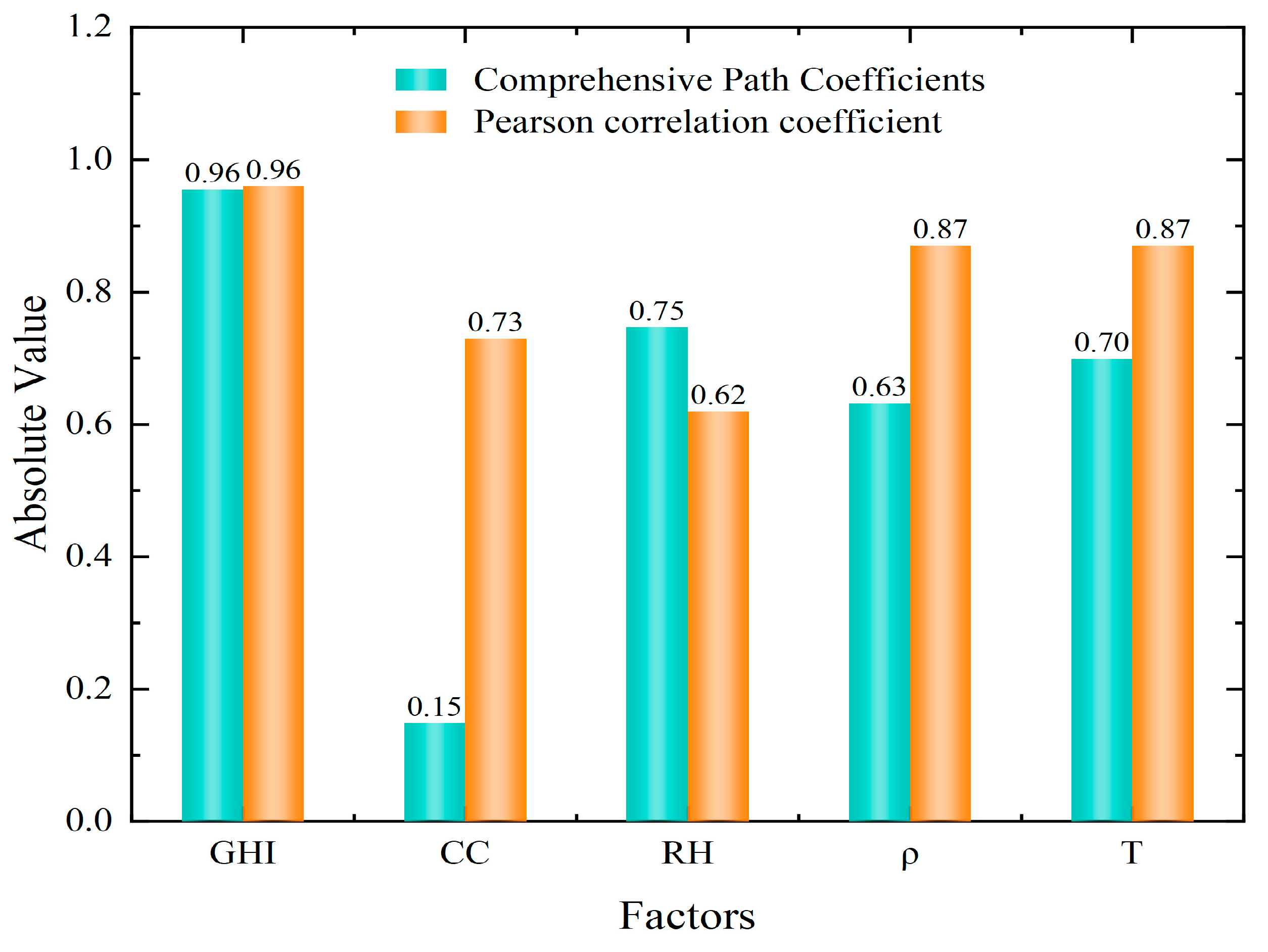
The correlation coefficient ignores the validity of the link between two or more factors and the power of a solar power station and only describes the linear relationship between the power of a photovoltaic power station and any one of the five elements. We therefore created a route graph model between the power of the solar power station and the different parameters, with the exception of wind speed, in order to quantitatively assess the effect of the interaction of the various factors on the power, as shown in Figure 3. The power of the solar power plant is directly influenced by the ambient temperature and the intensity of the sun’s radiation (GHI and T). The energy source for solar power generation is specifically solar radiation, and the power of a photovoltaic power plant is strongly positively correlated with the global horizontal irradiance (GHI). The working temperature of a photovoltaic panel is referred to as the ambient temperature. The photovoltaic conversion efficiency for a solar panel decreases as the ambient temperature increases [43]. The atmospheric density (ρ), relative humidity, and cloud cover have direct and indirect effects on the global horizontal irradiance (GHI). The local atmospheric movement and atmospheric density are also tightly connected. It is difficult for water vapor to condense when there is a strong vertical downdraft in a region with a high air density. The majority of bright days cause the intensity of the solar radiation to rise (GHI). The likelihood of precipitation rises with the increasing relative humidity (RH) and cloud cover (CC), and the decreasing impact of cloud cover on the global horizontal irradiance (GHI) is inversely connected with the global horizontal irradiance (GHI). According to Table 1, the relative humidity (RH) and global horizontal irradiance (GHI), which differ from the Pearson correlation coefficient (r) values in Figure 7, are the primary variables impacting the power of the photovoltaic power plant, in terms of the path coefficients. The interplay of these elements results in this effect.

5.3. Determination of the Weights for a Short-Term Prediction Model for a Photovoltaic Power Station

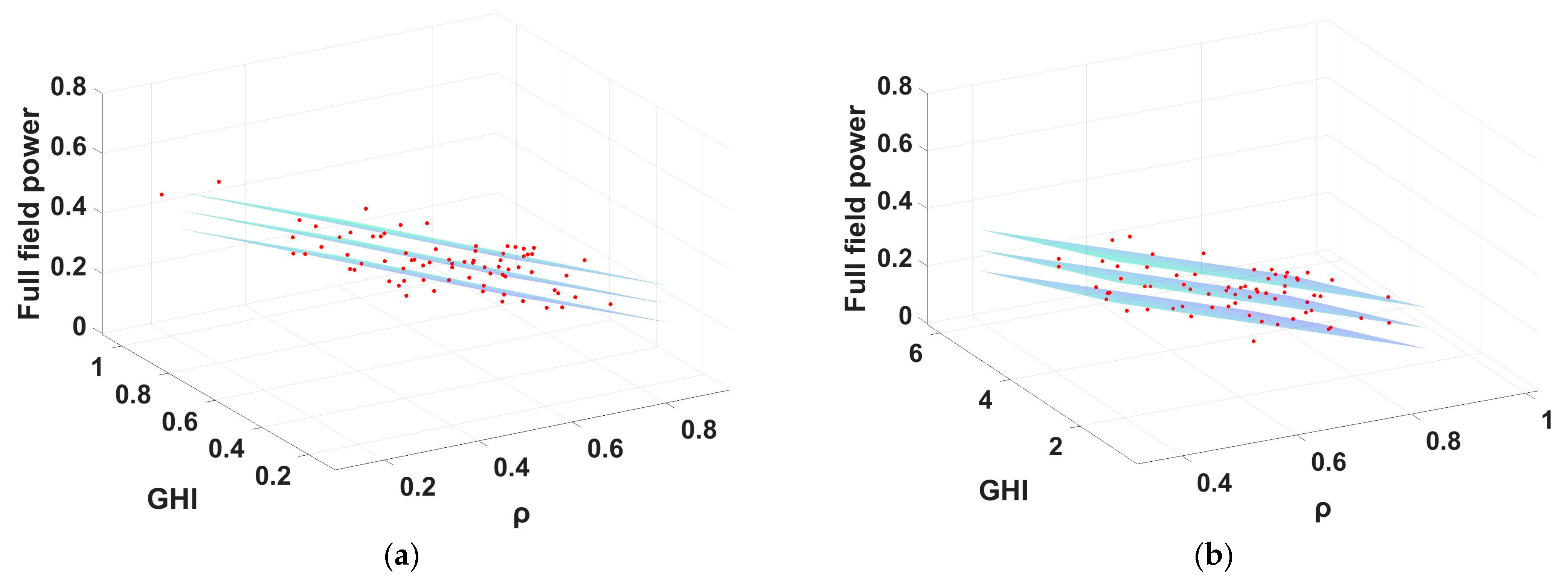
We use the support vector regression (SVR) model to make short-period predictions of the photovoltaic power plant power based on five factors except for wind speed. We created numerous weighting modules to ascertain the effect of the weights of the aforementioned elements on the power of the photovoltaic power station since the different factors contribute differently. In order for the point furthest from the hyperplane to have the shortest distance to the plane, the ideal hyperplane must be found using the SVR model. The data points outside of the two parallel planes are estimated as losses at the same time that the two parallel planes with $\frac{1}{2}{‖w‖}^2$ distance from the hyperplane are formed. We carried out a series of experiments to investigate the construction of numerous weighting modules based on the iterative convergence process of SVR. As illustrated in Figure 8, we performed multiple regression on GHI (x), ρ(y), and photovoltaic power (z) using the SVR model Figure 8a. In a different set of tests, we gave the atmospheric density (ρ) a lot of weight. The visualization outcomes for the ideal hyperplane of SVR after weighting are displayed in Figure 8b. In order to investigate the change in the correlation (R²) between the GHI (x), ρ(y), and photovoltaic power (Z) before and after weighting, we projected the SVR model before and after weighting, as shown in Figure 8, on planes X-O-Z and Y-O-Z, as shown in Figure 9.

The data points in Figure 9 are projections of the points within the two parallel hyperplanes in Figure 9 on planes X-O-Z and Y-O-Z, in accordance with the SVR loss function’s calculation concept. Figure 9 demonstrates that the correlation between ρ and the photovoltaic power decreases after the weighted regression of ρ. The overall model prediction accuracy is increased, as is the connection between the GHI and photovoltaic power. This effect is caused by the fact that we added a lot of weight to ρ, which somewhat contributes to the power of the photovoltaic power station. Actually, this was performed to expand the y-axis and the y-coordinate of the data points in the SVR prediction model in Figure 9 so that the data points are closer to the hyperplane, which is more favorable for model convergence and reduced loss. As a result, the distance weighting approach is employed in the SVR prediction model to provide more weight to the components with low contribution degrees, which can increase the model’s predictive accuracy [44,45].

6. Conclusions

In this study, six parameters that impact the output of a photovoltaic power station were chosen in order to assess both their individual and combined effects on the output of a solar power plant. A weighted prediction model for a photovoltaic power plant was also built. Firstly, the correlation analysis was used to evaluate the impact of the individual influencing elements on the power of the solar power plant, and then the SEM was used to quantify the overall impact of the aforementioned influencing factors. The findings indicate that parameters such as wind speed, which has a minimal effect on the output of a photovoltaic power station, can almost be ignored, and are outweighed by factors such as global horizontal irradiance (GHI), ambient temperature (T), and atmospheric density (ρ). Secondly, a multiple weighting module was constructed using the Mahalanobis distance to determine the weights of the aforementioned factors (with the exception of wind speed) in the power prediction task for a photovoltaic power station, based on the degree to which they contributed to the power of the photovoltaic power station. Finally, the SVR model based on PSO was used to perform the short-term weighted prediction of the photovoltaic power, and the impact of the various weighting modules on the model’s predictive accuracy was compared. The findings demonstrate that the significant variables with high correlation coefficients, such as solar radiation intensity, can partially reflect or forecast the output of a photovoltaic power plant (GHI). In addition, the factors with low correlation coefficients are crucial for estimating the photovoltaic power and enhancing the predictive ability. The prediction accuracy can be increased even further by the interplay of the many elements. Finally, a multivariate weighted module based on the Mahalanobis distance was constructed to calculate the weight of each factor in the photovoltaic power prediction task, after taking into account the univariate and multivariate effectiveness and evaluating the contribution level of each factor to the photovoltaic power station. The outcomes demonstrate that the suggested multiple weighted regression model can surpass the multiple regression model in terms of prediction accuracy. Compared to multiple regression (PSO-SVR), the R² showed an improvement of 7.2%, the SSE showed a 10.7% improvement, and the RMSE showed a 2.2% improvement.

The short-term weighted prediction model for a photovoltaic power station proposed in this paper can accurately predict the short-term photovoltaic output power by inputting the solar irradiation intensity and meteorological conditions to obtain the fluctuating and intermittent photovoltaic output power variations. Photovoltaic output power monitoring systems are widely used in the field of photovoltaic power station management because they can remotely monitor the grid-connected photovoltaic power station [46]. In grid-connected power generation, it is necessary to keep an eye on the power of the photovoltaic power station. Based on this, our proposed photovoltaic output power short-term weighted prediction model combined with the photovoltaic output power monitoring system will serve for the monitoring and management of grid-connected PV power generation, which will help to maintain the stability and security of the power grid.

This research only offers a method for creating a multiple weighted regression model based on the field measurements of ground stations, and preliminarily explores the effect of the prospective variables on the power of a solar power plant. Future field tests are required to evaluate the proposed model’s performance and accuracy in real-world settings. The link between these elements and photovoltaic power may differ, and the efficacy of these factors may vary from site to site, which is another problem worth considering. In order to enhance the effectiveness of the forecasting, the structure of the route graph model could be modified to examine the impact of various combinations of factors on the power of a solar power plant. The accuracy of the prediction could also be increased by taking into account the input sequence of past measurement data.

References

1. Jia, Y.; Alva, G.; Fang, G. Development and Applications of photovoltaic—Thermal systems: A review. Renew. Sustain. Energy Rev. 2019, 102, 249–265. [Google Scholar] [CrossRef]
2. Hernandez-Callejo, L.; Gallardo-Saavedra, S.; Alonso-Gomez, V. A review of photovoltaic systems: Design, operation and maintenance. Sol. Energy 2019, 188, 426–440. [Google Scholar] [CrossRef]
3. Ahmed, R.; Sreeram, V.; Mishra, Y.; Arif, M.D. A review and evaluation of the state-of-the-art in PV solar power forecasting: Techniques and optimization. Renew. Sustain. Energy Rev. 2020, 124, 109792. [Google Scholar] [CrossRef]
4. Feng, J.; Chen, M.; Li, Y.; Zhong, J. An Implementation of Full Cycle Strategy Using Dynamic Blending for Rapid Refresh Short-range Weather Forecasting in China. Adv. Atmos. Sci. 2021, 38, 943–956. [Google Scholar] [CrossRef]
5. Li, Y.; Wan, Y.; Xiao, J.; Zhu, Y. Prediction of Photovoltaic Power Generation Based on POS-BP Neural Network. In Bio-Inspired Computing: Theories and Applications: 14th International Conference, BIC-TA 2019, Zhengzhou, China, 22–25 November 2019, Revised Selected Papers, Part II 14; Springer: Singapore, 2020. [Google Scholar]
6. Brusco, G.; Burgio, A.; Menniti, D.; Pinnarelli, A.; Sorrentino, N.; Vizza, P. Quantification of Forecast Error Costs of Photovoltaic Prosumers in Italy. Energies 2017, 10, 1754. [Google Scholar] [CrossRef] [Green Version]
7. Gueymard, C. Critical analysis and performance assessment of clear sky solar irradiance models using theoretical and measured data. Sol. Energy 1993, 51, 121–138. [Google Scholar] [CrossRef]
8. Feng, Y.; Gong, D.; Zhang, Q.; Jiang, S.; Zhao, L.; Cui, N. Evaluation of temperature-based machine learning and empirical models for predicting daily global solar radiation. Energy Convers. Manag. 2019, 198, 111780. [Google Scholar] [CrossRef]
9. Yang, L.; Gao, X.; Hua, J.; Wu, P.; Li, Z.; Jia, D. Very Short-terms Surface Solar Irradiance Forecasting Based On FengYun-4 Geostationary Satellite. Sensors 2020, 20, 2606. [Google Scholar] [CrossRef] [PubMed]
10. Gueymard, C.A. REST2: High-performance solar radiation model for cloudless-sky irradiance, illuminance. Sol. Energy 2008, 82, 272–285. (In Chinese) [Google Scholar] [CrossRef]
11. Voyant, C.; Notton, G.; Kalogirou, S.; Nivet, M.L.; Paoli, C.; Motte, F.; Fouilloy, A. Machine learning methods for solar radiation forecasting: A review. Renew. Energy 2017, 105, 569–582. [Google Scholar] [CrossRef]
12. Shen, Y.; Wei, H.; Zhu, T.; Zhao, X.; Zhang, K. A Data-driven Clear Sky Model for Direct Normal Irradiance. J. Phys. Conf. 2018, 1072, 012004. [Google Scholar] [CrossRef] [Green Version]
13. Heo, J.; Song, K.; Han, S.; Lee, D.E. Multi-channel convolutional neural network for integration of meteorological and geographical features in solar power forecasting. Appl. Energy 2021, 295, 117083. [Google Scholar] [CrossRef]
14. Luo, Z.; Fang, F. Prediction of Photovoltaic Power Generation Based on PSO-RNN and SVR Model. In Proceedings of the 2019 International Conference on Sensing, Diagnostics, Prognostics, and Control (SDPC), Beijing, China, 15–17 August 2019. [Google Scholar]
15. Pierro, M.; Bucci, F.; De Felice, M.; Maggioni, E.; Moser, D.; Perotto, A.; Spada, F.; Cornaro, C. Multi-Model Ensemble for day ahead prediction of photovoltaic power generation. Sol. Energy 2016, 134, 132–146. [Google Scholar] [CrossRef]
16. Aslam, M.; Lee, J.M.; Kim, H.S.; Lee, S.J.; Hong, S. Deep Learning Models for Long-Term Solar Radiation Forecasting Considering Microgrid Installation: A Comparative Study. Energies 2019, 13, 147. [Google Scholar] [CrossRef] [Green Version]
17. Xiong, T.; Pu, Z.; Yi, J.; Tao, X. Fixed-time observer based adaptive neural network time-varying formation tracking control for multi-agent systems via minimal learning parameter approach. IET Control Theory Appl. 2020, 14, 1147–1157. [Google Scholar] [CrossRef]
18. Yang, Z.; Mourshed, M.; Liu, K.; Xu, X.; Feng, S. A novel competitive swarm optimized RBF neural network model for Short-terms solar power generation forecasting. Neurocomputing 2020, 397, 415–421. [Google Scholar] [CrossRef]
19. Grace, J.B. Structural Equation Modeling and Natural Systems: Principles of Estimation and Model Assessment; Cambridge University Press: Cambridge, UK, 2006. [Google Scholar]
20. Carrera, B.; Min, K.S.; Jung, J.Y. PVHybNet: A Hybrid Framework for Predicting Photovoltaic Power Generation Using Both Weather Forecast and Observation Data. IET Renew. Power Gener. 2020, 14, 2192–2201. [Google Scholar] [CrossRef]
21. Sun, Y.; Venugopal, V.; Brandt, A.R. Short-terms solar power forecast with deep learning: Exploring optimal input and output configuration. Sol. Energy 2019, 188, 730–741. [Google Scholar] [CrossRef]
22. Chairperson, C. In Situ and Solar Radiometer Measurements of Atmospheric Aerosols in Bozeman, Montana. Ph.D. Thesis, Montana State University—Bozeman, College of Engineering, Bozeman, MT, USA, 2011. [Google Scholar]
23. Muthén, B. A General structural equation Model with dichotomous, ordered categorical, and continuous latent variable indicators. Psychometrika 1984, 49, 115–132. [Google Scholar] [CrossRef] [Green Version]
24. Lefcheck, J.S. piecewise SEM: Piecewise structural equation modelling in r for ecology, evolution, and systematics. Methods Ecol. Evol. 2016, 7, 573–579. [Google Scholar] [CrossRef]
25. Mardani, A.; Streimikiene, D.; Zavadskas, E.K.; Cavallaro, F.; Nilashi, M.; Jusoh, A.; Zare, H. Application of Structural Equation Modeling (SEM) to solve environmental sustainability problems: A comprehensive review and meta-analysis. Sustainability 2017, 9, 1814. [Google Scholar] [CrossRef] [Green Version]
26. Zhu, T.; Guo, Y.; Wang, C.; Ni, C. Inter-hour forecast of solar radiation based on the structural equation model and ensemble model. Energies 2020, 13, 4534. [Google Scholar] [CrossRef]
27. De Maesschalck, R.; Jouan-Rimbaud, D.; Massart, D.L. The Mahalanobis distance. Chemom. Intell. Lab. Syst. 2000, 50, 1–18. [Google Scholar] [CrossRef]
28. Zhu, W.; Ma, H.; Cai, G.; Chen, J.; Wang, X.; Li, A. Research on PSO-ARMA-SVR Short-terms Electricity Consumption Forecast Based on the Particle Swarm Algorithm. Wirel. Commun. Mob. Comput. 2021, 2021, 6691537. [Google Scholar] [CrossRef]
29. Ghazvinian, H.; Mousavi, S.F.; Karami, H.; Farzin, S.; Ehteram, M.; Hossain, M.S.; Fai, C.M.; Hashim, H.B.; Singh, V.P.; Ros, F.C.; et al. Integrated support vector regression and an improved particle swarm optimization-based model for solar radiation prediction. PLoS ONE 2019, 14, e0217634. [Google Scholar] [CrossRef] [Green Version]
30. Abo-Khalil, A.G. Maximum Power Point Tracking for a PV System Using Tuned Support Vector Regression by Particle Swarm Optimization. J. Eng. Res. 2020, 8, 139–152. [Google Scholar] [CrossRef]
31. Soleimani, H.; Kannan, G. A hybrid particle swarm optimization and genetic algorithm for closed-loop supply chain network design in large-scale networks. Appl. Math. Model. 2015, 39, 3990–4012. [Google Scholar] [CrossRef]
32. Fadhillah, M.F.; Lee, S.; Lee, C.W.; Park, Y.C. Application of Support Vector Regression and Metaheuristic Optimization Algorithms for Groundwater Potential Mapping in Gangneung-si, South Korea. Remote Sens. 2021, 13, 1196. [Google Scholar] [CrossRef]
33. Kennedy, J.; Eberhart, R. Particle Swarm Optimization. In Proceedings of the ICNN95-International Conference on Neural Networks, Perth, WA, Australia, 27 November–1 December 1995. [Google Scholar]
34. Hosseini, M.; Naeini, S.A.; Dehghani, A.A.; Khaledian, Y. Estimation of soil mechanical resistance parameter by using particle swarm optimization, genetic algorithm and multiple regression methods. Soil Tillage Res. 2016, 157, 32–42. [Google Scholar] [CrossRef]
35. Fu, C.; Gan, S.; Yuan, X.; Xiong, H.; Tian, A. Determination of Soil Salt Content Using a Probability Neural Network Model Based on Particle Swarm Optimization in Areas Affected and Non-Affected by Human Activities. Remote Sens. 2018, 10, 1387. [Google Scholar] [CrossRef] [Green Version]
36. Li, Y.; Tian, Y.; Ouyang, Z.; Wang, L.; Xu, T.; Yang, P.; Zhao, H. Analysis of soil erosion characteristics in small watersheds with particle swarm optimization, support vector machine, and artificial neuronal networks. Environ. Earth Sci. 2009, 60, 1559–1568. [Google Scholar]
37. Wei, Q.; Nurmemet, I.; Gao, M.; Xie, B. Inversion of Soil Salinity Using Multisource Remote Sensing Data and Particle Swarm Machine Learning Models in Keriya Oasis, Northwestern China. Remote Sens. 2022, 14, 512. [Google Scholar] [CrossRef]
38. Basak, D.; Srimanta, P.; Patranbis, D.C. Support Vector Regression. Neural Inf. Process. Lett. Rev. 2007, 11, 203–224. [Google Scholar]
39. Mohanty, R.; Kale, P.G. Influence of Wind Speed on Solar PV Plant Power Production—Prediction Model Using Decision-Based Artificial Neural Network. In Advances in Computational Intelligence and Communication Technology: Proceedings of CICT 2019; Springer: Singapore, 2021. [Google Scholar]
40. Hersbach, H. Decomposition of the Continuous Ranked Probability Score for Ensemble Prediction Systems. Wea Forecast. 2000, 15, 559–570. [Google Scholar] [CrossRef]
41. Yang, D. A universal benchmarking method for probabilistic solar irradiance forecasting. Sol. Energy 2019, 184, 410–416. [Google Scholar] [CrossRef]
42. Xu, R.; Chen, H.; Sun, X. Short-term photovoltaic power forecasting with weighted support vector machine. In Proceedings of the 2012 IEEE International Conference on Automation and Logistics (ICAL), Zhengzhou, China, 15–17 August 2012. [Google Scholar] [CrossRef]
43. Hughes, B.R.; Cherisa, N.; Beg, O. Computational study of improving the efficiency of photovoltaic panels in the UAE. World Acad. Sci. Eng. Technol. 2011, 5, 33–42. [Google Scholar]
44. Han, X.; Clemmensen, L. On Weighted Support Vector Regression. Qual. Reliab. Eng. Int. 2015, 30, 891–903. [Google Scholar] [CrossRef]
45. Xu, Y.; Wang, L. A weighted twin support vector regression. Knowl. Based Syst. 2012, 33, 92–101. [Google Scholar] [CrossRef]
46. Patcharaprakiti, N.; Premrudeepreechacharn, S. Maximum power point tracking using adaptive fuzzy logic control for grid-connected photovoltaic system. In Proceedings of the Power Engineering Society Winter Meeting, Boston, MA, USA, 1–5 May 2005. [Google Scholar] [CrossRef]
Figure 1. Structural equation model construction process.
Sustainability 15 10808 g001
Figure 2. Structure of the short-cycle weighted prediction model for a photovoltaic power station.
Sustainability 15 10808 g002
Figure 3. Path graph model between the photovoltaic power plant and the five factors (GHI is global horizontal irradiance, ρ is atmospheric density, CC is cloud cover, RH is relative humidity, T is ambient temperature, Full-field power is the photovoltaic power station, and the box number is the normalized path coefficient of each variable.).
Sustainability 15 10808 g003
Figure 4. Performance evaluation of short-term prediction model for photovoltaic output power ((a) is the prediction result of neural network regression; (b) is the prediction result of PSO-RFR; (c) is the prediction result of PSO-LightGBM; (d) is the prediction result of PSO-SVR; (e) is the prediction result of short-term weighted prediction model for the photovoltaic power station).
Sustainability 15 10808 g004
Figure 5. Statistical chart of the hourly wind speed in Changzhou during the study period.
Sustainability 15 10808 g005
Figure 6. Pearson correlation coefficients for every two different variables. (GHI is global horizontal irradiance, ρ is atmospheric density, CC is cloud cover, WS is wind speed, RH is relative humidity, T is ambient temperature, and full-field power is the photovoltaic power station power).
Sustainability 15 10808 g006
Figure 7. Histogram of the comprehensive path coefficients and Pearson correlation coefficient (r) values for the five factors affecting a photovoltaic power station.
Sustainability 15 10808 g007
Figure 8. Comparison of the models before and after weighting. ((a) shows the convergence result of unweighted SVR, and (b) shows the convergence result of ρ-weighted SVR).
Sustainability 15 10808 g008
Figure 9. Comparison of the model projections before and after weighting. ((a,c) are projections of the convergence results of unweighted SVR, and (b,d) are projections of the convergence results of ρ-weighted SVR).
Sustainability 15 10808 g009