Article

Impact of Climate Change on the Spatio-Temporal Variation in Groundwater Storage in the Guangdong–Hong Kong–Macao Greater Bay Area

1
Plateau Atmosphere and Environment Key Laboratory of Sichuan Province, Chengdu University of Information Technology, Chengdu 610225, China
2
State Key Laboratory of Numerical Modeling for Atmospheric Sciences and Geophysical Fluid Dynamics, Institute of Atmospheric Physics, Chinese Academy of Sciences, Beijing 100029, China
3
Key Laboratory of Hydrometeorological Disaster Mechanism and Warning of Ministry of Water Resources, Nanjing University of Information Science & Technology, Nanjing 210044, China
*
Author to whom correspondence should be addressed.
Sustainability 2023, 15(14), 10776; https://doi.org/10.3390/su151410776
Submission received: 29 April 2023 / Revised: 1 July 2023 / Accepted: 5 July 2023 / Published: 10 July 2023

Abstract

:
The Guangdong–Hong Kong–Macao Greater Bay Area (GBA) is one of the world’s four major bay areas. Groundwater is indispensable in ensuring water supply for human production and living, as well as social and economic development. Studying the spatial–temporal variation in groundwater storage (GWS) and exploring the impact of climate change on GWS is of great significance for water resource management in the GBA. In this work, we conducted a simulation using the Community Land Model version 5.0 (CLM5.0) and combined it with Gravity Recovery and Climate Experiment (GRACE) data to calculate GWS in the GBA. In addition, based on the multiple linear regression model, we quantitatively assessed the effects of different climate factors on the change in GWS in the GBA. Comparisons with groundwater wells, automatic weather stations, and satellite observations demonstrated reasonable results. Our results showed that precipitation and evapotranspiration are the main factors affecting the change in GWS in the GBA. Precipitation dominates GWS anomaly changes in areas where wetting and precipitation vary drastically, such as the northern part of Foshan. GWS is closely related to evapotranspiration, in which water and heat changes are significant.

1. Introduction

The Guangdong–Hong Kong–Macao Greater Bay Area (GBA) is one of the world’s four major bay areas. It is one of China’s most economically and culturally developed regions and plays an important strategic role in its development. The sound development of the GBA requires the support of adequate water resources. Due to the developed internal river networks and broad drainage basins, the GBA is rich in water resources. However, the spatio-temporal distribution of precipitation is uneven; as it is mainly concentrated in the period between April and September [1]. There are more water resources in mountainous areas than plain areas, in eastern areas than western areas, and in southeastern coastal areas than northwestern inland areas [2]. Given economic and social development and population growth, the distribution of social–economic productivity does not match the allocation of water resources. Many cities in the GBA face severe water shortage, with the per capita water resources (the average amount of available water per person) below the threshold for severe water shortage (500 m3) in populated areas [3], such as Hong Kong, Macao, Shenzhen, Zhuhai, and Guangzhou [4]. The massive discharge of waste water also leads to water shortages caused by pollution [3,5,6], further reducing water resource availability. Under the combined effects of the above factors, water resource shortages, water security, and water environmental pressures have become increasingly prominent issues in the GBA.
Groundwater is a water resource stored in subsurface pore spaces and defined channels [7], and it is the largest available store of global freshwater [8]. It can meet agricultural and industrial water demands and is vital for human production activities. The GBA has a great potential for groundwater exploitation because of its hydrogeological characteristics (see Section 2.1 for details), while the third series reconstruction layer sequence, karst layer, and cataclastic rocks constitute rich groundwater layers [9,10]. In addition, water demand in the Pearl River Basin, including the GBA, is mainly met by a huge system of dams and reservoirs [11], and the aquifers in GBA are underutilized. The development and utilization of groundwater can effectively solve the contradiction between water supply and demand related to future economic growth. Therefore, studying the spatio-temporal variation in groundwater water storage (GWS) in the GBA is of great significance.
The method of estimating GWS based on observation wells is limited due to the sparse number of in situ observation stations and the high cost of human and material resources, which makes it difficult to provide long-term and large-scale measurements of GWS changes. Gravity Recovery and Climate Experiment (GRACE) gravity satellite data [12] provide an effective approach for monitoring changes in terrestrial water storage (TWS) on a large scale. Land surface models (LSMs) can be used to study changes in hydrological components, such as soil moisture (SM), snow water, and surface water [13,14,15]. Combined with a water balance equation (see Section 2.4.1 for details) and LSMs [16], GWS changes can be separated from changes in TWS [17]. Bhanja et al. (2016) combined GRACE and a LSM to estimate the GWS anomaly (GWSA) in 12 major river basins in India; the estimated results were in good agreement with most observational estimates [18]. Using GRACE and the Global Land Data Assimilation System dataset, Liu et al. (2022) analyzed the changes in GWS in the Taihang Mountains in the period 2003–2016 and the dominant driving factors influencing changes [19]. Alghafli et al. (2023) used GRACE and Global Land Data Assimilation System products to calculate the changes in GWS from 2010 to 2016, comparing these changes with a time series of groundwater observations to verify the effectiveness of GRACE [20]. Meanwhile, the Community Land Model (CLM), Noah model, and variable infiltration capacity model have also been used to assess groundwater recharge [20]. Feng et al. (2013) utilized GRACE and four hydrological models to estimate groundwater depletion in North China, and the results were consistent with those sourced from monitoring well stations [21]. Feng et al. (2018) used GRACE data with hydrological models and LSMs, including CLM, to estimate GWS changes in China’s three major aquifers [22]. The results showed that GRACE could be used to estimate GWS changes, and CLM simulated the lowest magnitudes of SM storage (SMS) rates among the four models used. Rateb et al. (2020) [23] compared GRACE with groundwater level monitoring data and eight hydrologic models and LSMs, finding that LSMs were more responsive to changes in GWS than the hydrologic models in six aquifer regions in the southwestern and south–central United States. This result occurred because most LSMs do not include surface water storage (SWS) or human intervention [23].
The above studies illustrate that combining GRACE and a LSM is an effective way to estimate GWS changes. However, these studies have mainly focused on hot spots of GWS loss, such as the North China Plain [24], Colorado River Basin [17], Alberta [25], and American High Plain Aquifer [26]. There are few studies on GWS changes in the GBA, and there have been a lack of satellite monitoring data analyses in recent years. In this work, we estimated the GWS changes in the GBA from 2003 to 2016 based on the water mass budget (Equation (1)) using GRACE satellite data and land surface model CLM version 5.0 (CLM5.0). The hydrologic variables in the water mass budget, including snow water storage (SnWS), canopy water storage (CWS), and SMS, were calculated using CLM5.0. In addition, the influencing factors of GWS change in the GBA were analyzed based on a multiple linear regression method.

2. Materials and Methods

2.1. Study Area

The GBA is located in the south subtropical zone along the southeastern coast of Guangdong Province, China, extending from 21° N to 25° N and 111° E to 116° E. It covers an area of approximately 5.6 × 10⁴ km2 and includes nine municipalities directly administered by the governments of Guangzhou, Shenzhen, Foshan, Zhaoqing, Dongguan, Zhongshan, Huizhou, Jiangmen, and Zhuhai, as well as the special administrative regions of Hong Kong and Macao (Figure 1). It is located in a tropical monsoon region and has an annual average temperature range of 21–23 °C. The average annual precipitation is 1300–2400 mm [27]. Under the influence of typhoons that occur in the East China Sea, rainfall increases from the northwest to the southeast. The annual relative humidity is 75–85% [2]. The hydrogeological characteristic of the GBA mainly comprises the Quaternary sequence and upper Mesozoic intrusion unit. The Quaternary sequence is characterized by anisotropic and heterogeneous groundwater flow [28]. Below the Quaternary sequence, the third series reconstruction layer sequence, karst layer, and cataclastic rocks constitute rich groundwater layers [9,11].

2.2. Model

This study used CLM5.0 to simulate the hydrological components in the GBA in the period 2003–2016. CLM5.0 is the land surface model of the Community Earth System Model [29]. Based on previous versions, CLM5.0 incorporated new changes in photosynthesis and stomatal conductance, improved the CLM’s snow physics, added MOSART for river routing, described external inputs to the nitrogen cycle, and updated the CROP option. [29,30,31]. In CLM5.0, the vertical soil moisture transport was calculated via the mass conservation equation and Darcy’s law [29,32].

2.3. Datasets

2.3.1. Meteorological Forcing Data

The Chinese Meteorological Forcing Dataset (CMFD) was adopted, which was developed by the Institute of Tibetan Plateau Research, the Chinese Academy of Sciences, for the study of land surface processes in China [33,34,35]. The CMFD was obtained from Princeton reanalysis data, National Aeronautics and Space Administration/Global Energy and Water Cycle Experiment–Surface Radiation Budget radiation data, Tropical Rainfall Measuring Mission precipitation data, and Global Land Data Assimilation System data, and it was combined with the observation data from nearly 700 meteorological stations managed by the China Meteorological Administration via ANU-Spline statistical interpolation. The time span of CMFD is 1979–2018, the time resolution is 3 h, and the spatial resolution is 0.1° × 0.1°. It contains seven near-surface meteorological element variables, including the air temperature at 2 m above the ground, surface pressure, specific humidity, the wind speed at 10 m above the ground, downward short-wave radiation, downward long-wave radiation, and the precipitation rate.

2.3.2. Soil Properties Data

The soil properties data were based on a gridded Chinese soil properties dataset developed by ShangGuan et al. (2013) [36]. Its spatial resolution is 30 arcs × 30 arcs, covering an area of approximately 1 km × 1 km, including eight soil layers. In the dataset, 9000 soil profiles from the second National Soil Survey (1979–1985) of the China Soil Map (1:1,000,000) were used [37], and the spatial distribution of soil properties was deduced via the polygonal linkage method [38].

2.3.3. Plant Functional Types Data

The plant functional types data used in the model comprised the plant functional types map in China with a resolution of 1 km released by the Cold and Arid Regions Data Center [39]. These data were obtained by applying the climate rules for land cover and plant functional type conversion proposed by Bonan et al. (2002) to the Multi-Source Integrated Chinese Land Cover map [39,40,41,42,43]. The Multi-Source Integrated Chinese Land Cover data include Chinese land use, Chinese plant types, Chinese glacier distribution, Chinese marsh wetland, and land cover.

2.3.4. GRACE Satellite Data

GRACE is a twin satellite that was launched by NASA and the German Aerospace Centre in 2002 to monitor changes in the Earth’s gravity [12]. The GRACE data mainly estimate the monthly mean global gravity field data based on the accurate K-band ranging measurements of the K-band ranging system [44]. These measurements were obtained from the release datasets of the Center for Space Research at the University of Texas [45,46]. The spatial resolution of the data was 0.25° × 0.25°, the temporal resolution was months, and the time span was 2003–2016.

2.3.5. In Situ Groundwater Table Depth Data

To validate the estimation of GWS changes, the monthly groundwater table depth data of 26 in situ observation stations were collected for the period 2005–2016 from the Geological Environment Monitoring Institute of the China Geological Survey. Outliers that deviated from the average by three standard deviations were removed, and the values were averaged from these 26 in situ observation stations. This analysis was performed because of the large number of missing observations (15 in situ observation stations with more than 45% missing data). It should be noted that since the 0.25° resolution of the estimated GWSA can only reflect the average state within a grid cell, few observations were available and they were clustered together with similar hydrogeological information. Thus, we used the average value of observations to validate the estimated GWS with 0.25° resolution. In addition, there are few fast recharge systems available in the locations of the groundwater table depth stations used in this study [47]; thus, it was reasonable to utilize the above processing method for groundwater table depth data. Most in situ observation stations were located in the northwestern area of the GBA, and there were a few in situ observation stations in the southeastern area. The locations of the sites are shown by black triangular dots in Figure 1.

2.3.6. In Situ SM Data

Monthly SM data collected from six in situ observation stations from September 2015 to December 2016 were used to evaluate the simulated SM, as provided by the China Meteorological Administration. The six in situ observation stations were Conghua, Nanhai, Dongguan, Guangning, Taishan, and Longmen, as shown by the red dots in Figure 1. The SM values at different depths of the model grid cells were interpolated to the depths for each station via a linear interpolation method.

2.3.7. ESA CCI SM Data

As a further evaluation, SM data version 6.1 for the period 2003–2016 from the European Space Agency’s Climate Change Initiative (ESA CCI) were used [48]. These data were obtained using a combination of active and passive microwave sensors that measured microwave radiation emitted or reflected from the surface. The spatial resolution of the data was 0.25°, and the temporal resolution was 1 day. For the convenience of comparison and verification, the monthly average of the time dimension was obtained.

2.4. Study Methods

2.4.1. Calculation of GWSA

The TWS anomaly (TWSA), which was provided by GRACE, was the anomaly of TWS relative to the long-term (2004–2009) mean, and it was a vertically integrated hydrologic variable [49] that consisted of GWSA, SnWS anomaly (SnWSA), SMS anomaly (SMSA), CWS anomaly (CWSA), and SWS anomaly (SWSA). The filtering process used to smoothen the GRACE data weakened the geophysical signal, using a set of scaling factors for signal recovery [50,51], though this method ignored some of the effects of surface water [52]. In addition, most of the LSMs did not contain SWS [23]. Therefore, GWSA was calculated as follows [17,25]:
GWSA = TWSA − SnWSA − CWSA − SMSA
where, SnWSA, CWSA, and SMSA were calculated using CLM5.0. All storage anomalies were those values relative to the mean value of the period 2004–2009 (Figure 2).

2.4.2. Multiple Linear Regression

Multiple linear regression was used to evaluate the contribution of different meteorological elements to the GWS. Due to the problem of different units and scales between variables, each variable required standardization.
The equation for standard deviation normalization was as follows:
x = x μ σ
where x is the variable that needs to be standardized, x is the standardized variable, μ is the mean value of the variable, and σ is the standard deviation of the variable. After standardization, multiple linear regression was used to calculate the corresponding regression coefficient for each variable.
The regression equation was as follows [53,54]:
y = a 1 x 1 + a 2 x 2 + a 3 x 3 + b
where, y is the monthly average value of GWS at a given grid cell, and x1, x2, and x3 are the monthly average precipitation, evapotranspiration, and temperature of each grid cell, respectively. a1, a2, and a3 are regression coefficients, and b is the residual term. The monthly average precipitation and the monthly average temperature of each grid cell were derived using CMFD forcing data, and the monthly average evapotranspiration was obtained via CLM5.0 simulation.
The contribution of precipitation, temperature, and evapotranspiration to GWS was quantified via the following equation [54]:
C o n t r i b u t i o n i = a i i 3 a i
where a i is the contribution coefficient of each variable to GWS.

2.4.3. Mann–Kendall (MK) Test

This study used the MK trend test to determine whether the trend was significant [55,56,57]. The MK trend test could be used for mutation testing, significance analysis, and evaluating the monotonicity or variability in time series. Its advantages were that the data did not need to obey a specific distribution, allowed missing data, were not disturbed by a few outliers, and had strong applicability. Given a time series with the length of n, the null hypothesis of no trend assumed that the time series were independently distributed. The standardized test statistic was calculated as follows:
Z = ( S 1 )   /   V a r ( S )         if   S > 0 0                                                                     if   S = 0 ( S + 1 )   /   V a r ( S )         if   S < 0
where the test statistic S is calculated as follows:
S = i = 1 n 1 j = i + 1 n s g n ( x j x i )
where a positive value of S indicates an increasing trend, while a negative value indicates a decreasing trend. The sgn(x) is a symbolic function, and xi and xj represent the values of sequence i and j, respectively. When n > 8 [55,56], S is approximately normally distributed, and variance Var(S) is calculated as follows:
V a r ( S ) = n ( n 1 ) ( 2 n + 5 ) k = 1 p q k ( q k 1 ) ( 2 q k + 5 ) 18
where qk is the number of data in the tied group, and p is the number of tied groups.
The null hypothesis of no trend was rejected when the absolute value was larger than the theoretical value, albeit within the statistical significance level concerned (this figure was set to 0.05 in this study).

2.4.4. Root Mean Square Error (RMSE)

Following previous studies [58,59], several statistical indicators are commonly used to assess the accuracy of simulated SM: the RMSE, Pearson’s correlation coefficient (R), and Taylor’s skill score (TSS).
The RMSE was calculated as follows [60]:
R M S E = 1 N i = 1 N ( D A i D P i ) 2
where N is the number of samples. D A i and D P i   are the observed and predicted values, respectively. In this study, this equation could be used to verify the reliability of simulated SM.

2.4.5. Pearson’s Correlation Coefficient (R)

The R was used to analyze the correlation between simulated SM and observed SM, as well as the correlation between the respective variables and dependent variables of the multiple linear regression. The R was calculated as follows:
r X Y = i = 1 n ( X X ¯ ) ( Y Y ¯ ) i = 1 n ( X X ¯ ) 2 · i = 1 n ( Y Y ¯ ) 2
where n is the number of samples, X ¯   is the mean value of variable X, and Y ¯   is the mean value of variable Y. The value range of r X Y   is [–1,1]. When r X Y > 0, X and Y variables were positively linearly correlated; when <0, X and Y variables were negatively linearly correlated.

2.4.6. Mean Squared Error (MSE)

The MSE was calculated as follows [61]:
M S E = 1 n i = 1 n ( Y i Y ^ i ) 2
where n is the number of samples, and Yi and Y ^ i are the observed and predicted values, respectively. The smaller the MSE value, the more accurate the prediction result. In this study, this equation was used to verify the reliability of simulated SM.

2.4.7. TSS

TSS [62] was used to quantitatively evaluate model performance and calculated as follows [59,63]:
T S S = 4 ( 1 + R ) 4 ( σ f + 1 / σ f ) 2 ( 1 + R 0 ) 4
where σf is the ratio of standard deviation between simulations and observations, R is the correlation coefficient between simulations and observations, and R0 is the maximum possible correlation coefficient. The value of TSS ranges from 0 to 1, with higher values reflecting better performance.

2.5. Experimental Design

The CMFD was used to drive the CLM5.0. The GBA surface data were obtained using the CLM5.0 tools, and the tools replaced the original soil properties and plant functional type data for each grid cell with high-resolution data (details in Section 2.3.2 and Section 2.3.3 [36,39]) based on the plural sampling method. The simulated domain range was 21° N–25° N and 110.5° E–115.5° E, with a spatial resolution of 5 km and a time step of 1800 s from 2003 to 2016. A cyclically spin-up run was conducted for 50 years to balance out the hydrological process before the formal simulation. Combined with the hydrological components from the CLM5.0 simulation and GRACE data, the GWSA from 2003 to 2016 relative to the average value from 2004 to 2009 were calculated in mm.

3. Results

3.1. Spatio-Temporal Distribution of GWSA

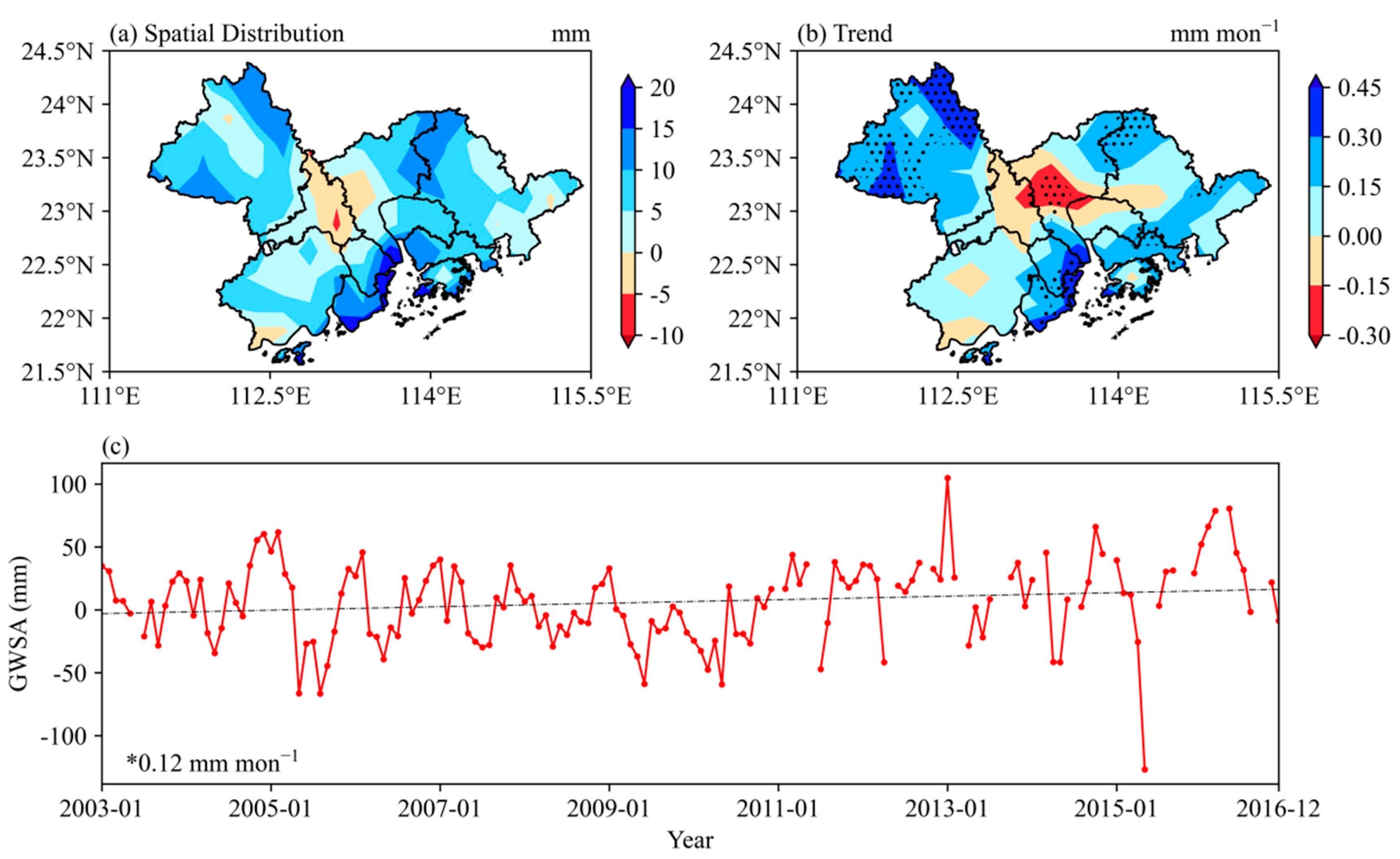
Regarding the spatial distribution (Figure 3a), the GWSA of the GBA was negative in the central region, generally positive in the surrounding areas, and slightly negative in the southwest region, though the absolute value was relatively small. The trends of change (Figure 3b) and spatial distribution were similar, showing a decreasing trend in the central region and an increasing trend in surrounding areas. The northwestern and northeastern areas are primarily mountainous, with high altitudes and fast groundwater flow rates, and are affected by short-term climate change; therefore, the changes here were more significant. In the central part of the GBA, increased precipitation results in increased evapotranspiration, and the groundwater shows a significant decreasing trend. Figure 3c shows the temporal variation in GWSA. Moreover, GWSA in the GBA showed a slowly increasing trend from 2003 to 2016, with a growth rate of 0.12 mm/month (Figure 3c). Moreover, the uncertainty in the estimated GWS in the GBA mainly originated from the SM due to the small values of SnWSA and CWSA, according to Equation (1). The relative deviation in the simulated SM from the ESACCI data is approximately 14.66%, which directly indicates that the SM simulated in this study is reasonable and indirectly indicates the reasonableness of the estimated GWS.

3.2. Verification of SM

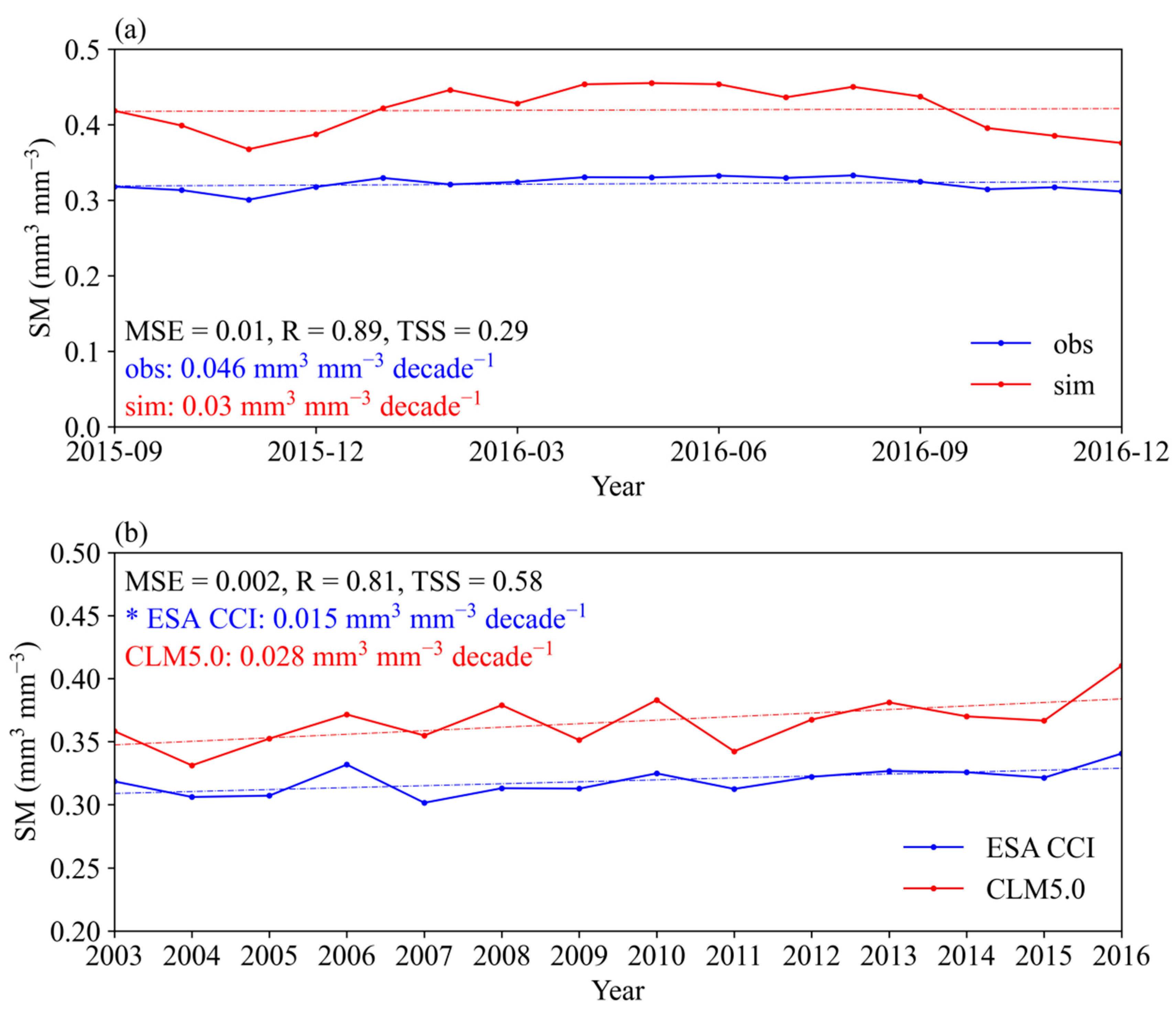
To verify the accuracy of the model simulation, the simulated SM was compared to the observed SM (Figure 4a). The observed SM was used for the top 100 cm (10, 20, 30, 40, 50, 60, 80, and 100 cm). The first nine soil layers (1, 4, 9, 16, 26, 40, 58, 80, and 106 cm) of the simulated SM were interpolated to the SM at the corresponding observed depth. The weighted averages of the observed and simulated SMs for the top 100 cm were then calculated and compared. The R and MSE between the observed and simulated results (see Figure 4a) indicated a reasonable simulated SM. The trend of the simulated SM was 0.03 mm3/mm3/decade, which was similar to the trend of observed SM (0.046 mm3/mm3/decade).
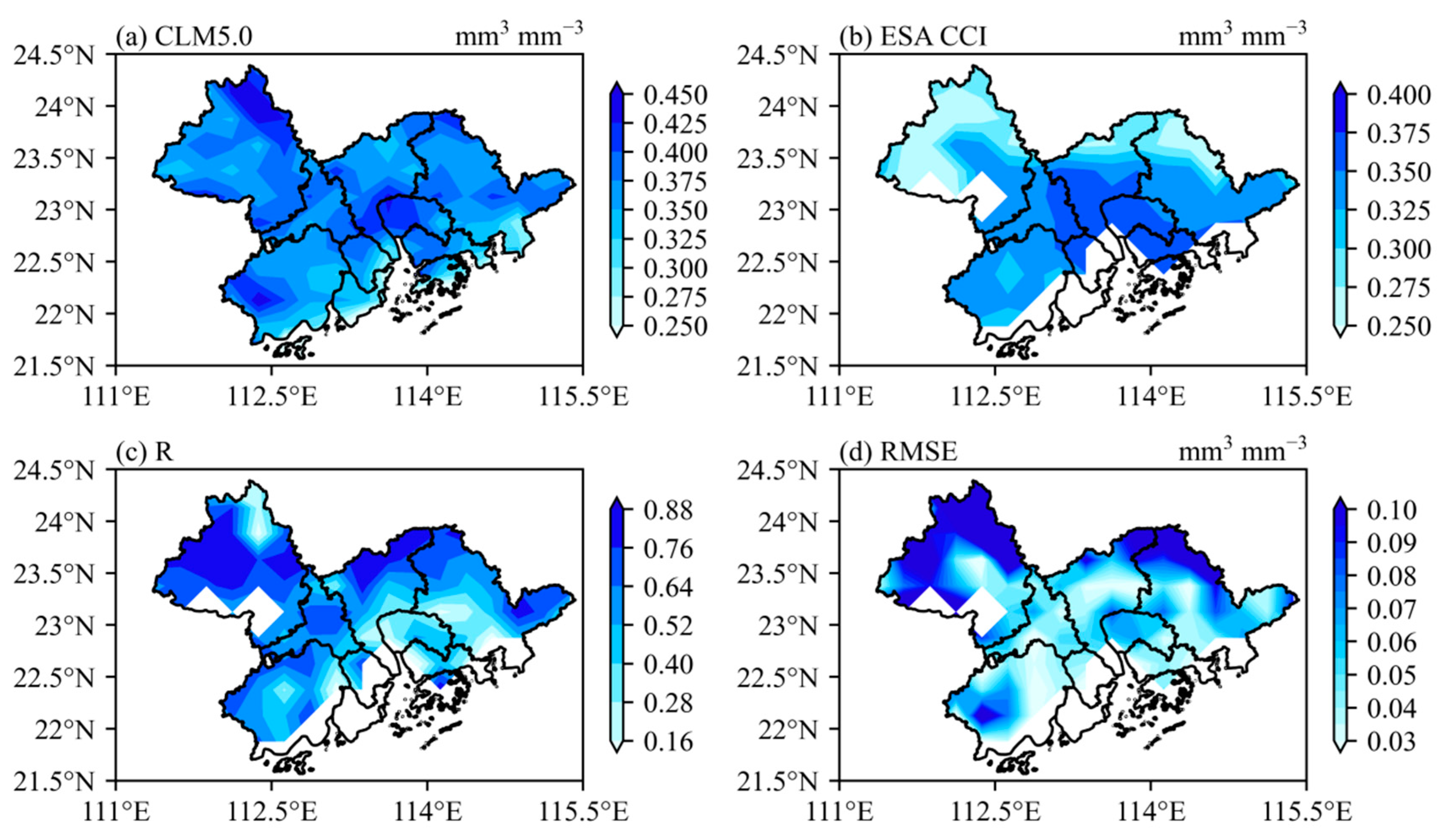
The SM simulated using CLM5.0 and ESA CCI SM v6.1 data were compared and verified via the spatial scale. The weighted average value of the first three soil layers (thickness: 2 cm, 4 cm, and 6 cm; weights: 0.2, 0.4, and 0.4) of the CLM5.0 simulation was compared to that of the ESA CCI. Figure 5 shows that the simulated SM was higher than the ESA CCI in central GBA, but lower in the northwestern mountainous area, as well as the northeastern and southwestern areas. The spatial distribution between the simulated SM and ESA CCI was consistent (Figure 5a,b). Figure 5c,d shows the R and RMSE of SM simulated via CLM5.0 and the SM simulated via ESA CCI, respectively. There was a good correlation between both methods (Table 1). From 2003 to 2016, the SM of the GBA increased at a rate of 0.028 mm3/mm3 per decade and peaked in 2016 (Figure 4b). Overall, CLM5.0 could reasonably reflect the SM changes in the GBA.

3.3. Verification of GWSA

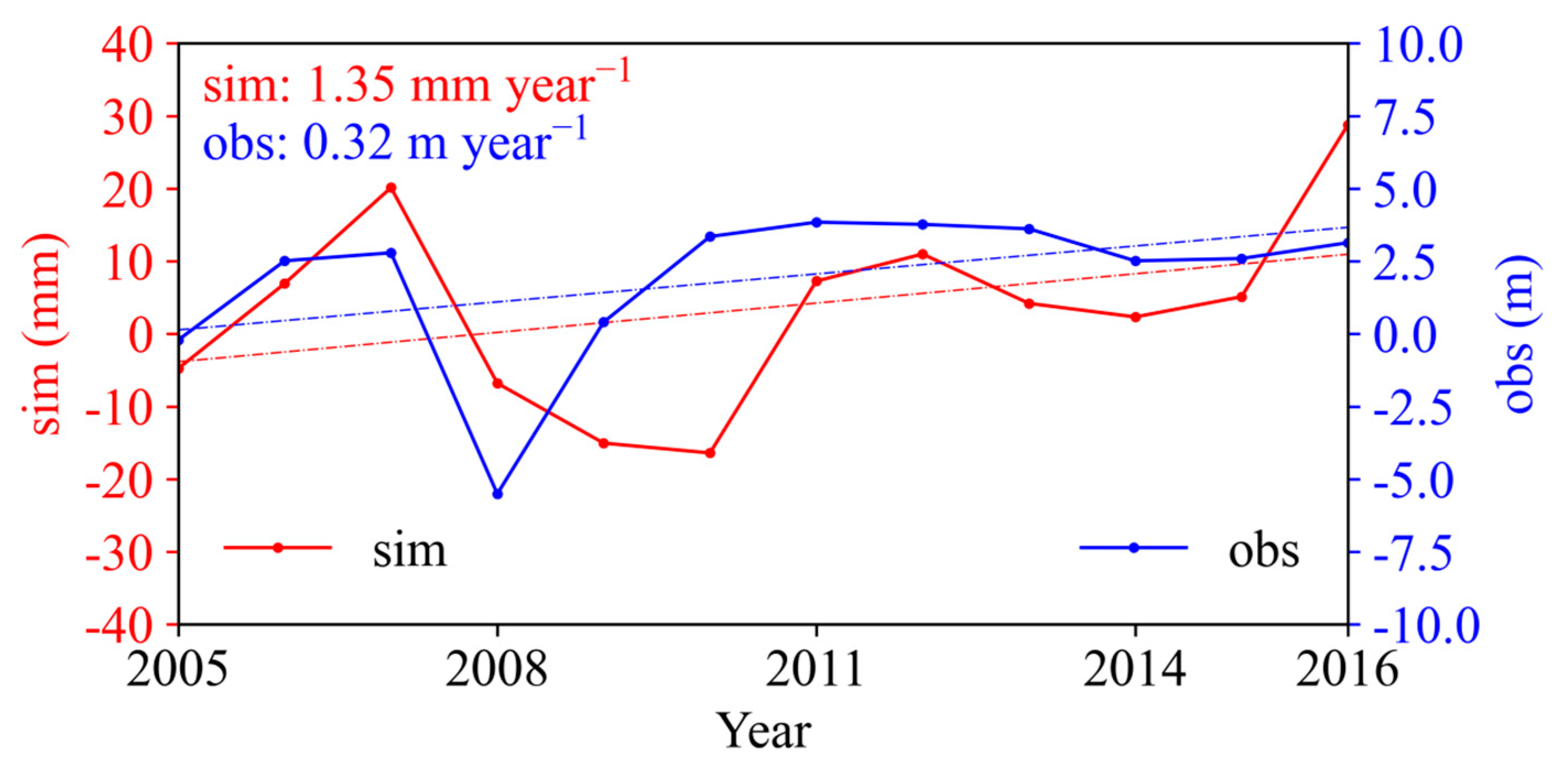
The calculated GWSA was then compared to the observed values (Figure 6). To validate the estimated GWSA, we processed the observed groundwater table depth data in the following way. Firstly, outliers that were more than three times the standard deviation of the average value were eliminated. We then calculated the average value of observations, and finally, for consistency with the estimated GWSA, the observation anomaly relative to the 2005–2009 mean value was calculated (considering the available time series of observed data). A detailed explanation of the reasonableness of the processing method is given in Section 2.3.5. Next, the observed groundwater table depth anomaly was converted to the groundwater level anomaly by multiplying it by −1. The observed station was at a single point, and the resolution of the calculated GWSA was 0.25°; some uncertainties may have occurred due to the mismatch between the different resolutions. Thus, the calculated GWSA was compared to the observed groundwater level anomaly from the GBA average value perspective. We noted that the groundwater level data obtained from the water wells needed to be multiplied by specific yields to estimate the GWS [19]. Due to unreliable specific yield data, GWSA was verified by comparing the annual variation and trends of observed and calculated data.
There was an increasing trend of GWSA in the GBA over the period 2005–2016. The consistency between the trend of calculated GWSA and the observed data indicates that the combination of GRACE and CLM5.0 simulation can better reflect variations in GWSA. However, differences occurred in 2009, which were possibly caused by the mismatch between the calculated GWSA and the groundwater table depth observations. Since the actual area of the GBA is 56,000 km2, with strong heterogenic hydrological and geological conditions, GRACE data with a coarse resolution cannot capture these heterogeneities (the original spatial resolution of GRACE data is 1° × 1° [64]). There was also a large gap in spatial scale between the sites and GRACE data, and the spatial scale mismatch caused part of the difference [65]. Although GRACE data are filtered on the balance of accuracy and spatial resolution to reduce noise interference [66], signal loss also increases with decreasing noise interference, meaning that smaller spatial scales will result in more errors, especially those associated with the leakage problem [67].

3.4. Spatio-Temporal Variation in Precipitation, Temperature, and Evapotranspiration

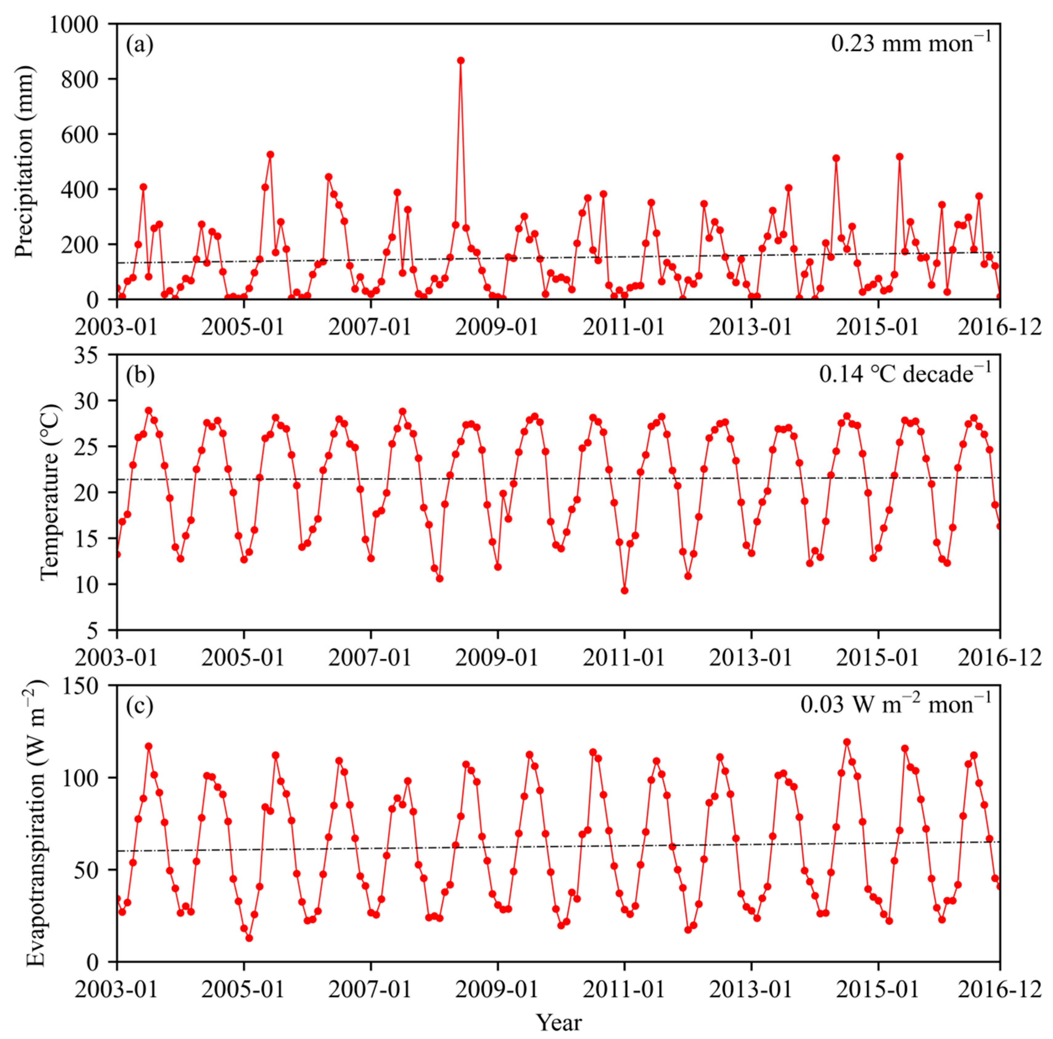
Precipitation and evapotranspiration affect the availability of water infiltration in the subsurface as recharge, and temperature is associated with evapotranspiration [68]. To deepen understanding of GWSA changes in the GBA, changes in climate factors were investigated. Figure 7 shows the monthly time series of precipitation, temperature, and evapotranspiration in the GBA from 2003 to 2016. As it has a critical role in the water cycle, precipitation was low in 2004 and had a prominent peak in 2008 (Figure 7). Xu et al. (2021) indicated a drought in the Pearl River Basin in 2004 [69]. However, large-scale floods occurred in 2005, 2006, and 2008 [69], which correspond with peak precipitation values.
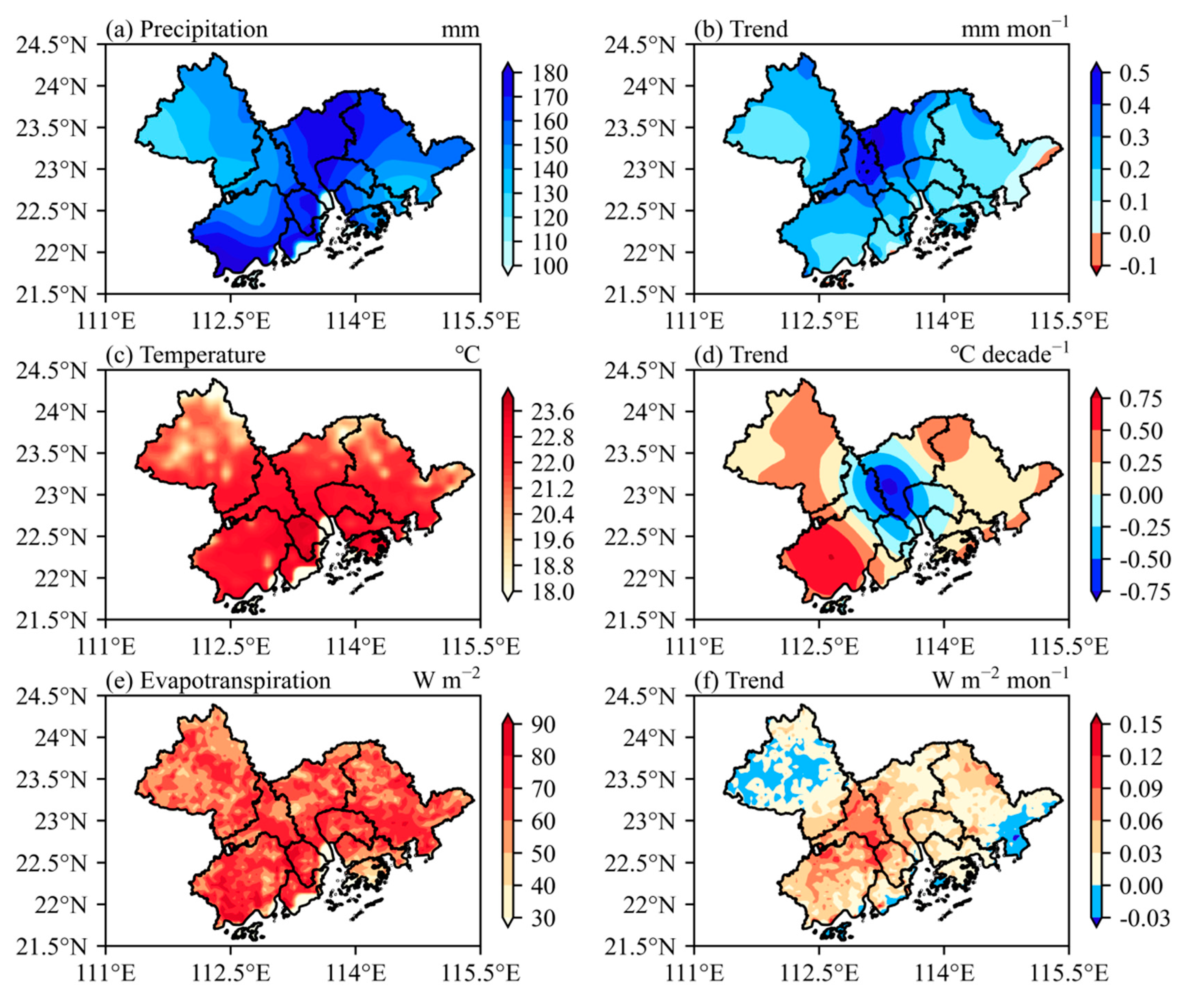
Regarding the spatial distribution (Figure 8a,c,e), precipitation was higher in the east and lower in the west, as well as higher on the southeast coast than in the northwest inland area, which is similar to the findings of Cao et al. (2021) [2]. The temperature in the Pearl River estuary is higher than that in other areas, especially in places such as Guangzhou, where the temperature differs significantly from the surrounding areas, and the average summer temperature can reach 31 °C. The spatial distribution of evapotranspiration was not apparent, though high-value areas were primarily located in the regions with greater precipitation and higher temperatures.
Figure 8b shows that precipitation had an increasing trend over a wide area in the GBA, especially in the central region, with a maximum increase of 0.51 mm/month. Only the precipitation in the eastern part of the GBA had a decreasing trend of −0.14 mm/month. Temperature variation (Figure 8e) was generally slight. However, there was a cooling trend in the central region of the GBA of approximately 0.8 °C per decade, while the temperature typically increased in other regions, with an increasing trend of up to 0.83 °C per decade in the southwestern GBA. Evapotranspiration (Figure 8f) increased in the central region of the GBA at 0.17 W/m2 per month, while it decreased in the northwestern and southeastern regions at −0.04 W/m2 per month. From the time series perspective, there was a slight increase in precipitation and evapotranspiration, as well as some fluctuations in temperature, but no significant trends, which is similar to a previous study’s results [27].

3.5. Contributions of Climatic Factors to GWSA

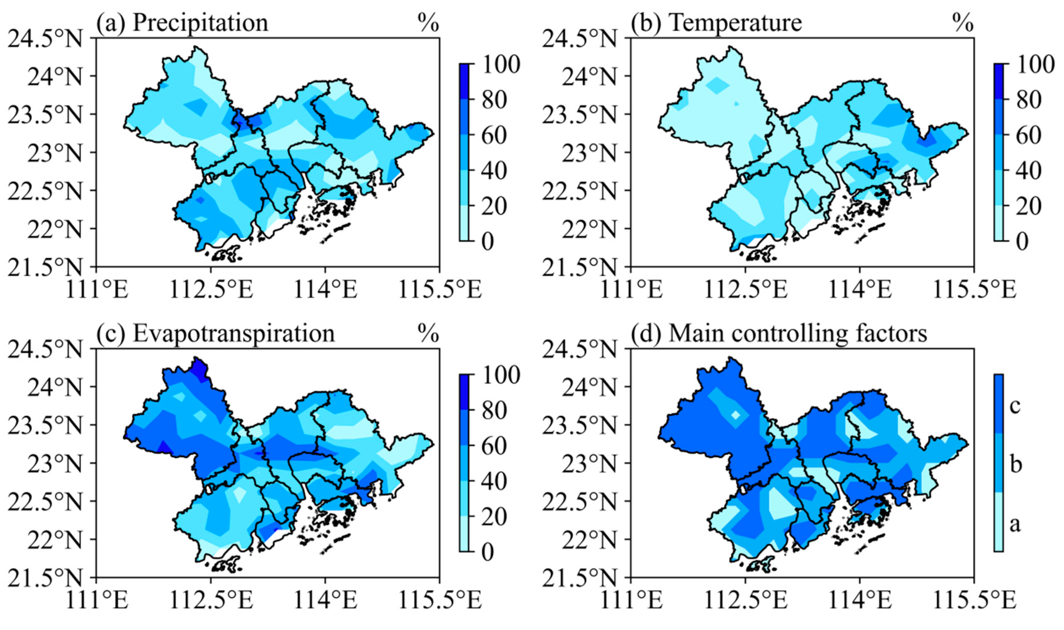
GWSA, precipitation, temperature, and evapotranspiration were standardized for each grid cell. A multiple linear regression model was established that used the standardized GWSA as the dependent variable and precipitation, temperature, and evapotranspiration as the independent variables. The contributions of each climatic factor to GWS were calculated based on Equation (1). Figure 9 shows that the average contribution of evapotranspiration was 58.53%, while average contributions of precipitation and temperature were 26.83% and 14.63%, respectively. The GWS of the GBA was mainly controlled via precipitation and evapotranspiration, while temperature had a relatively slight effect. The precipitation-controlled regions were located in the wetting areas of the GBA, while evapotranspiration-controlled regions were located in the northwestern mountainous area and the central region of the GBA.
The northwest region of the GBA is mountainous and composed of basement units. The permeability decreases rapidly with increasing depth, and the precipitation is low. The precipitation mainly replenishes the river with surface runoff, and the remaining water enters the soil, which is greatly affected by evapotranspiration. Therefore, evapotranspiration has a significant effect on GWS. In the southwestern region of the GBA, precipitation was high, and temperature increased significantly; therefore, GWSA in the southwest of GBA was closely related to evapotranspiration and temperature. In northern Foshan and western Guangzhou, precipitation increased significantly; hence, precipitation in this region played a dominant role in GWS changes. In the central region of the GBA, precipitation and temperature increased significantly, and evapotranspiration also changed drastically under sufficient water–heat recharge. The significant decrease in GWS in this region was closely related to evapotranspiration. In the southeastern coastal area of the GBA, precipitation was high, and GWSA was not limited by moisture; therefore, the influence of evapotranspiration here was more pronounced. Overall, precipitation dominated GWSA changes in areas where wetting and precipitation varied drastically, such as northern Foshan. The GWS was closely related to evapotranspiration, where water and heat changes were significant.

4. Discussion

4.1. Model Performance and Uncertainty

Combined GRACE data and CLM5.0 simulation in this work were successfully applied to GWSA estimation in the GBA. Many factors will affect the accuracy of the estimation. The initial resolution of GRACE was 1° × 1°, and the area of each grid cell was approximately 10,000 km2 [45], while the area of the GBA was 56,000 km2. The coarse resolution of GRACE could lead to uncertainties for a small region. The leakage problem of GRACE could also influence the accuracy of TWSA. During GRACE data processing, mass changes in the study area were affected by mass changes outside of the area, an effect known as the leakage problem, which caused deviation in the retrieved TWSA [70,71].
In addition, the accuracy of meteorological data, land cover data, and model structure could lead to some bias in the simulation of hydrological components (e.g., SM) [72]. Since CLM5.0 is a land component used for climate simulations and does not fully consider geological information, there may be biases in the simulation of deep soils. Furthermore, the interpolation process introduces uncertainties during data processing because of the different resolutions between CLM5.0 simulations and GRACE.

4.2. Limitations

However, it should be noted that there are still some limitations. The impact of human activities needs to be considered when estimating the GWSA for smaller areas. According to the Pearl River Basin Water Resources Bulletin, the groundwater supply of several major cities in the GBA only accounts for 0.616% of the total water supply, which has a negligible impact on the GWSA. Considering that the primary purpose of this study was to estimate the changes in GWSA at a large scale, with the results showing that our approach is reasonable, the role of human activities was not further explored, though it is worth investigating in the future.
Future work could focus on the sustainable development and management of groundwater resources in the GBA; for example, the potential for groundwater extraction and changes in groundwater quality could be considered. Groundwater extraction potential is influenced by geological conditions, land use, topographic density, drainage density, slope, soil type, rainfall, elevation, and groundwater table fluctuations [73]. The hydrogeologic structure includes the hydro-lithologic characteristics of aquifers, which affect the variation in the groundwater table [74]. The suitability of groundwater for extraction is also related to groundwater quality, with pollutants from population growth and industrialization increasing the pressure on surface and groundwater [75]. Future studies could focus on strategies to address these aspects.

5. Conclusions

In this study, GRACE data were combined with the CLM5.0 simulation to calculate GWSA in the GBA, and the reliability of simulated SM and calculated GWSA was verified. Based on the multiple linear regression model, the influence of different climate factors on GWS changes in the GBA were quantitatively evaluated. The following findings were obtained.
The simulated SM using CLM5.0 was highly correlated with the observed data and could reflect the spatio-temporal changes in SM. A combination of GRACE data and CLM5.0 land surface simulation used to calculate GWSA in the GBA had a certain reliability. GWSA in the GBA showed a slowly increasing trend from 2003 to 2016, with a growth rate of 0.12 mm/month. Precipitation and evapotranspiration were the main factors affecting GWS changes in the GBA. Precipitation dominated GWSA changes in areas where wetting and precipitation varied drastically, such as northern Foshan and western Guangzhou. GWS was closely related to evapotranspiration in regions with significant water and heat changes.

Author Contributions

Conceptualization, Q.H., L.W. and B.J.; data collection, L.W.; data analysis, Q.H.; formal analysis, Q.H. and L.W.; methodology, Q.H., L.W., B.J., X.L. and Q.P.; writing—original draft; Q.H., reviewing and editing, L.W. and B.J. All authors have read and agreed to the published version of the manuscript.

Funding

This work was jointly supported by the National Natural Science Foundation of China (42205176), the Youth Innovation Promotion Association CAS (2021073), the China Postdoctoral Science Foundation (2022M723095), the Open Foundation of the Key Laboratory of Hydrometeorological Disaster Mechanism and Warning of the Ministry of Water Resources (HYMED202202), and the National Key Scientific and Technological Infrastructure project “Earth System Science Numerical Simulator Facility” (EarthLab).

Institutional Review Board Statement

Not applicable.

Informed Consent Statement

Not applicable.

Data Availability Statement

Data are available on request.

Acknowledgments

The CMFD dataset was provided by the National Tibetan Plateau Data Center (http://data.tpdc.ac.cn, accessed on 4 July 2023). The soil properties dataset was provided by the Land–Atmosphere Interaction Research Group at Sun Yat-sen University (Data Description and Source: http://globalchange.bnu.edu.cn/research/soil2, accessed on 4 July 2023). The plant functional types dataset was provided by the Cold and Arid Regions Data Center (Data Description and Source: http://poles.tpdc.ac.cn/zh-hans/data/ab193a70-63a5-4df6-9bc1-d9b5ac5fb044/, accessed on 4 July 2023). The GRACE RL06 is available via the following link: http://www2.csr.utexas.edu/grace, accessed on 4 July 2023). The ESA CCI SM dataset was provided by the European Space Agency’s Climate Change Initiative (Data Description and Source: https://climate.esa.int/en/odp/#/project/soil-moisture, accessed on 4 July 2023). All data were presented in the netCDF4 format.

Conflicts of Interest

The authors declare that they have no known competing financial interest or personal relationship that could have appeared to influence the work reported in this paper.

References

  1. Deng, F.; Yang, Y.; Zhao, E.-G.; Xu, N.; Li, Z.; Zheng, P.; Han, Y.; Gong, J. Urban Heat Island Intensity Changes in Guangdong–Hong Kong–Macao Greater Bay Area of China Revealed by Downscaling MODIS LST with Deep Learning. Int. J. Environ. Res. Public Health 2022, 19, 17001. [Google Scholar] [CrossRef] [PubMed]
  2. Cao, J.; Xia, R.; Tang, Z.; Zhao, L.; Wang, Z.; Luan, S.; Wang, S. Groundwater resources in Guangdong–Hong Kong–Macao Greater Bay Area and its development potential. Geol. China 2021, 48, 1075–1093, (In Chinese with English abstract). [Google Scholar]
  3. Wang, Y.; Huang, C.; Wu, G.; Wang, W. Status and Challenges of Water Resources and Supply in the Guangdong–Hong Kong–Macao Greater Bay Area (GBA) of China. Water Cycle 2022, 3, 65–70. [Google Scholar] [CrossRef]
  4. Cheng, L.; Song, S.; Xie, Y. Evaluation of Water Resources Utilization Efficiency in Guangdong Province Based on the DEA–Malmquist Model. Front. Environ. Sci. 2022, 10, 819693. [Google Scholar] [CrossRef]
  5. Wang, X.; Liu, L.; Qin, J. Integrated Model Framework for the Evaluation and Prediction of the Water Environmental Carrying Capacity in the Guangdong–Hong Kong–Macao Greater Bay Area. Ecol. Indic. 2021, 130, 108083. [Google Scholar] [CrossRef]
  6. Chen, Z.; Zhu, Z.; Yin, L.; Wei, S.; Deng, L. The Changing Water Quality Characteristics from Urban Drinking Water Sources in Guangdong, China. Water Resour. Manag. 2014, 29, 987–1002. [Google Scholar] [CrossRef]
  7. Brands, E.; Rajagopal, R.; Eleswarapu, U.; Li, P. Groundwater. Int. Encycl. Geogr. 2016, 3237–3253. [Google Scholar] [CrossRef]
  8. Cuthbert, M.O.; Gleeson, T.; Moosdorf, N.; Befus, K.M.; Schneider, A.; Hartmann, J.M.; Lehner, B. Global Patterns and Dynamics of Climate–Groundwater Interactions. Nat. Clim. Chang. 2019, 9, 137–141. [Google Scholar] [CrossRef]
  9. Cui, Q.; Shen, S.-L.; Shen, S.-L.; Wu, H.-N.; Yin, Z.-Y. Mitigation of Geohazards during Deep Excavations in Karst Regions with Caverns: A Case Study. Eng. Geol. 2015, 195, 16–27. [Google Scholar] [CrossRef]
  10. Lancia, M.; Su, H.W.; Tian, Y.; Xu, J.; Andrews, C.M.; Lerner, D.N.; Zheng, C. Hydrogeology of the Pearl River Delta, Southern China. J. Maps 2020, 16, 388–395. [Google Scholar] [CrossRef]
  11. Liu, X.; Shen, S.-L.; Cheng, W.S.; Horpibulsuk, S. Investigation of Hydraulic Parameters of a Weathered Mylonite Fault from Field Pumping Tests: A Case Study. Bull. Eng. Geol. Environ. 2016, 76, 1431–1448. [Google Scholar] [CrossRef]
  12. Tapley, B.D.; Bettadpur, S.; Ries, J.C.; Thompson, P.M.; Watkins, M.T. GRACE Measurements of Mass Variability in the Earth System. Science 2004, 305, 503–505. [Google Scholar] [CrossRef] [Green Version]
  13. Fan, Y.; Clark, M.R.; Lawrence, D.; Swenson, S.; Band, L.E.; Brantley, S.L.; Brooks, P.D.; Dietrich, W.D.; Flores, A.N.; Grant, G.E.; et al. Hillslope Hydrology in Global Change Research and Earth System Modeling. Water Resour. Res. 2019, 55, 1737–1772. [Google Scholar] [CrossRef] [Green Version]
  14. Ozdogan, M.; Rodell, M.; Beaudoing, H.K.; Toll, D.G. Simulating the Effects of Irrigation over the United States in a Land Surface Model Based on Satellite-Derived Agricultural Data. J. Hydrometeorol. 2010, 11, 171–184. [Google Scholar] [CrossRef]
  15. Xie, Z.; Liu, S.; Zeng, Y.; Gao, J.; Qin, P.; Jia, B.; Xie, J.; Liu, B.; Li, R.; Wang, Y.; et al. A High-Resolution Land Model with Groundwater Lateral Flow, Water Use, and Soil Freeze-Thaw Front Dynamics and Its Applications in an Endorheic Basin. J. Geophys. Res. Atmos. 2018, 123, 7204–7222. [Google Scholar] [CrossRef]
  16. Long, D.; Longuevergne, L.; Scanlon, B.R. Uncertainty in evapotranspiration from land surface modeling, remote sensing, and GRACE satellites. Water Resour. Res. 2014, 50, 1131–1151. [Google Scholar] [CrossRef] [Green Version]
  17. Scanlon, B.R.; Zhang, Z.; Reedy, R.C.; Pool, D.R.; Save, H.; Long, D.; Chen, J.; Wolock, D.M.; Conway, B.; Winester, D. Hydrologic implications of GRACE satellite data in the Colorado River Basin. Water Resour. Res. 2015, 51, 9891–9903. [Google Scholar] [CrossRef]
  18. Bhanja, S.N.; Mukherjee, A.; Ganguly, S.; Velicogna, I.; Famiglietti, J.S. Validation of GRACE based groundwater storage anomaly using in-situ groundwater level measurements in India. J. Hydrol. 2016, 543, 729–738. [Google Scholar] [CrossRef]
  19. Liu, M.; Pei, H.; Shen, Y. Evaluating dynamics of GRACE groundwater and its drought potential in Taihang Mountain Region, China. J. Hydrol. 2022, 612, 128156. [Google Scholar] [CrossRef]
  20. Alghafli, K.; Shi, X.; Sloan, W.; Shamsudduha, M.; Tang, Q.; Sefelnasr, A.; Ebraheem, A.A. Groundwater recharge estimation using in-situ and GRACE observations in the eastern region of the United Arab Emirates. Sci. Total Environ. 2023, 867, 161489. [Google Scholar] [CrossRef] [PubMed]
  21. Feng, W.; Zhong, M.; Lemoine, J.; Biancale, R.; Hsu, H.; Xia, J. Evaluation of groundwater depletion in North China using the Gravity Recovery and Climate Experiment (GRACE) data and ground-based measurements. Water Resour. Res. 2013, 49, 2110–2118. [Google Scholar] [CrossRef]
  22. Feng, W.; Shum, C.K.; Zhong, M.; Pan, Y. Groundwater Storage Changes in China from Satellite Gravity: An Overview. Remote Sens. 2018, 10, 674. [Google Scholar] [CrossRef] [Green Version]
  23. Rateb, A.; Scanlon, B.R.; Pool, D.R.; Sun, A.Y.; Zhang, Z.; Chen, J.; Clark, B.C.; Faunt, C.C.; Haugh, C.J.; Hill, M.C.; et al. Comparison of Groundwater Storage Changes from GRACE Satellites with Monitoring and Modeling of Major U.S. Aquifers. Water Resour. Res. 2020, 56, e2020WR027556. [Google Scholar] [CrossRef]
  24. Rodell, M.; Velicogna, I.; Famiglietti, J.S. Satellite-based estimates of groundwater depletion in India. Nature 2009, 460, 999–1002. [Google Scholar] [CrossRef] [Green Version]
  25. Bhanja, S.N.; Zhang, X.; Wang, J. Estimating long-term groundwater storage and its controlling factors in Alberta, Canada. Hydrol. Earth Syst. Sci. 2018, 22, 6241–6255. [Google Scholar] [CrossRef] [Green Version]
  26. McGuire, V.L. Water-Level Changes in the High Plains Aquifer, Predevelopment to 2009, 2007–2008, and 2008–2009, and Change in Water in Storage, Predevelopment to 2009; U.S. Geological Survey: Reston, VA, USA, 2011. [Google Scholar]
  27. Feng, X.; Zeng, Z.; He, M. A 20-year vegetation cover change and its response to climate factors in the Guangdong–Hong Kong–Macao Greater Bay Area under the background of climate change. Front. Ecol. Evol. 2023, 10, 1080734. [Google Scholar] [CrossRef]
  28. Huang, G.; Sun, J.; Zhang, Y.; Jing, J.; Liu, J. Distribution of Arsenic in Sewage Irrigation Area of Pearl River Delta, China. J. Earth Sci. 2011, 22, 396–410. [Google Scholar] [CrossRef]
  29. Lawrence, D.; Fisher, R.; Koven, C.D.; Oleson, K.W.; Swenson, S.; Bonan, G.B.; Collier, N.; Ghimire, B.; Van Kampenhout, L.; Kennedy, D.P.; et al. The Community Land Model Version 5: Description of New Features, Benchmarking, and Impact of Forcing Uncertainty. J. Adv. Model. Earth Syst. 2019, 11, 4245–4287. [Google Scholar] [CrossRef] [Green Version]
  30. Wang, L.; Xie, Z.; Jia, B.; Wang, Y.; Li, R.; Xie, J.; Chen, S.; Qin, P.; Shi, C. Recent Progress in the Land Surface Process Studies: A Case Study of CASLSM. Plateau Meteorol. 2021, 40, 1347–1363. [Google Scholar]
  31. Peng, Q.; Jia, B.; Lai, X.; Wang, L.; Huang, Q. Characteristics of near-surface soil freeze–thaw status using high resolution CLM5.0 simulations on the Tibetan Plateau. Atmos. Sci. Lett. 2023. [CrossRef]
  32. Dingman, S.L. Physical Hydrology, 2nd ed.; Prentice Hall: Upper Saddle River, NJ, USA, 2002. [Google Scholar]
  33. He, J.; Yang, K.; Tang, W.; Lu, H.; Qin, J.; Chen, Y.; Li, X. The first high-resolution meteorological forcing dataset for land process studies over China. Sci. Data 2020, 7, 25. [Google Scholar] [CrossRef] [Green Version]
  34. Yang, K.; He, J.; Tang, W.; Qin, J.; Cheng, C.C. On downward shortwave and longwave radiations over high altitude regions: Observation and modeling in the Tibetan Plateau. Agric. For. Meteorol. 2010, 150, 38–46. [Google Scholar] [CrossRef]
  35. Yang, K.; He, J. China Meteorological Forcing Dataset (1979–2018). A Big Earth Data Platform for Three Poles; National Tibetan Plateau Data Center: Beijing, China, 2019. [Google Scholar]
  36. Shangguan, W.; Dai, Y.; Liu, B.; Zhu, A.; Duan, Q.; Wu, L.; Ji, D.; Liang, X.; Yuan, H.; Zhang, Q.; et al. A China data set of soil properties for land surface modeling. J. Adv. Model. Earth Syst. 2013, 5, 212–224. [Google Scholar] [CrossRef]
  37. Liu, J.; Yang, Z.; Jia, B.; Wang, L.; Wang, P.; Zheng-Hui, X.; Shi, C. Elucidating Dominant Factors Affecting Land Surface Hydrological Simulations of the Community Land Model over China. Adv. Atmos. Sci. 2022, 40, 235–250. [Google Scholar] [CrossRef]
  38. Shangguan, W.; Dai, Y.; Liu, B.; Liang, X.; Yuan, H. A soil particle-size distribution dataset for regional land and climate modelling in China. Geoderma 2012, 171–172, 85–91. [Google Scholar] [CrossRef]
  39. Ran, Y.; Li, X. Plant Functional Types Map in China (1 km). A Big Earth Data Platform for Three Poles; National Tibetan Plateau Data Center: Beijing, China, 2019. [Google Scholar]
  40. Bonan, G.B.; Levis, S.; Kergoat, L.; Oleson, K.W. Landscapes as patches of plant functional types: An integrating concept for climate and ecosystem models. Glob. Biogeochem. Cycles 2002, 16, 5–23. [Google Scholar] [CrossRef] [Green Version]
  41. Ran, Y.; Li, X.; Lu, L. China Land Cover Classification at 1 km Spatial Resolution Based on a Multi-Source Data Fusion Approach. Adv. Earth Sci. 2009, 24, 192–203. [Google Scholar]
  42. Ran, Y.; Li, X.; Lu, L.; Li, Z.B. Large-scale land cover mapping with the integration of multi-source information based on the Dempster–Shafer theory. Int. J. Geogr. Inf. Sci. 2012, 26, 169–191. [Google Scholar] [CrossRef]
  43. Ran, Y.; Ma, H. 1 km Plant Functional Types Map over China in 2000. Remote Sens. Technol. Appl. 2016, 31, 827–832. [Google Scholar]
  44. Pie, N.; Bettadpur, S.; Tamisiea, M.E.; Krichman, B.; Save, H.; Poole, S.; Nagel, P.; Kang, Z.; Jacob, G.; Ellmer, M.; et al. Time Variable Earth Gravity Field Models from the First Spaceborne Laser Ranging Interferometer. J. Geophys. Res. Solid Earth 2021, 126, e2021JB022392. [Google Scholar] [CrossRef] [PubMed]
  45. Save, H.; Bettadpur, S.; Tapley, B.D. High-resolution CSR GRACE RL05 mascons. J. Geophys. Res. Solid Earth 2016, 121, 7547–7569. [Google Scholar] [CrossRef]
  46. Save, H. CSR GRACE and GRACE-FO RL06 Mascon Solutions v02. 2020. Available online: https://www2.csr.utexas.edu/grace/RL06_mascons.html (accessed on 4 July 2023).
  47. Lancia, M.; Yao, Y.; Andrews, C.M.; Wang, X.; Kuang, X.; Ni, J.; Gorelick, S.M.; Scanlon, B.R.; Wang, Y.; Zheng, C. The China groundwater crisis: A mechanistic analysis with implications for global sustainability. Sustain. Horiz. 2022, 4, 100042. [Google Scholar] [CrossRef]
  48. Preimesberger, W.; Scanlon, T.; Su, C.; Gruber, A.; Dorigo, W. Homogenization of Structural Breaks in the Global ESA CCI Soil Moisture Multisatellite Climate Data Record. IEEE Trans. Geosci. Remote Sens. 2021, 59, 2845–2862. [Google Scholar] [CrossRef]
  49. Khorrami, B.; Ali, S.; Gunduz, O. Investigating the Local-Scale Fluctuations of Groundwater Storage by Using Downscaled GRACE/GRACE-FO JPL Mascon Product Based on Machine Learning (ML) Algorithm. Water Resour. Manag. 2023, 37, 3439–3456. [Google Scholar] [CrossRef]
  50. Liu, R.; Zou, R.; Li, J.; Zhang, C.; Zhao, B.; Zhang, Y. Vertical Displacements Driven by Groundwater Storage Changes in the North China Plain Detected by GPS Observations. Remote Sens. 2018, 10, 259. [Google Scholar] [CrossRef] [Green Version]
  51. Rahaman, M.; Thakur, B.; Kalra, A.; Ahmad, S. Modeling of GRACE-Derived Groundwater Information in the Colorado River Basin. Hydrology 2019, 6, 19. [Google Scholar] [CrossRef] [Green Version]
  52. Sakumura, C.; Bettadpur, S.; Bruinsma, S. Ensemble prediction and intercomparison analysis of GRACE time-variable gravity field models. Geophys. Res. Lett. 2014, 41, 1389–1397. [Google Scholar] [CrossRef]
  53. Luo, X.; Jia, B.; Lai, X. Quantitative analysis of the contributions of land use change and CO2 fertilization to carbon use efficiency on the Tibetan Plateau. Sci. Total Environ. 2020, 728, 138607. [Google Scholar] [CrossRef]
  54. Wu, W.; Lo, M.; Wada, Y.; Famiglietti, J.S.; Reager, J.T.; Yeh, P.J.; Ducharne, A.; Yang, Z. Divergent effects of climate change on future groundwater availability in key mid-latitude aquifers. Nat. Commun. 2020, 11, 3710. [Google Scholar] [CrossRef]
  55. Mann, H. Non-parametric tests against trend. Econometrica 1945, 13, 245–259. [Google Scholar] [CrossRef]
  56. Kendall, M.G. Rank Correlation Methods. Biometrika 1957, 44, 298. [Google Scholar] [CrossRef]
  57. Sang, Y.-F.; Wang, Z.; Liu, C. Comparison of the MK Test and EMD Method for Trend Identification in Hydrological Time Series. J. Hydrol. 2014, 510, 293–298. [Google Scholar] [CrossRef]
  58. Wang, A.; Kong, X.; Chen, Y.; Ma, X. Evaluation of Soil Moisture in CMIP6 Multimodel Simulations over Conterminous China. J. Geophys. Res. Atmos. 2022, 127, e2022JD037072. [Google Scholar] [CrossRef]
  59. Qiao, L.; Zuo, Z.; Xiao, D. Evaluation of Soil Moisture in CMIP6 Simulations. J. Clim. 2022, 35, 779–800. [Google Scholar] [CrossRef]
  60. Pham, Q.B.; Kumar, M.; Di Nunno, F.; Elbeltagi, A.; Granata, F.; Islam, A.R.M.T.; Pal, S.; Nguyen, X.; Ahmed, A.; Anh, D.T. Groundwater level prediction using machine learning algorithms in a drought-prone area. Neural Comput. Appl. 2022, 34, 10751–10773. [Google Scholar] [CrossRef]
  61. Rabinowitz, L.; Rice, J.A. Mathematical Statistics and Data Analysis. Technometrics 1989, 31, 390. [Google Scholar] [CrossRef]
  62. Taylor, K.E. Summarizing Multiple Aspects of Model Performance in a Single Diagram. J. Geophys. Res. 2001, 106, 7183–7192. [Google Scholar] [CrossRef]
  63. Althoff, D.; Rodrigues, L.N. Goodness-of-Fit Criteria for Hydrological Models: Model Calibration and Performance Assessment. J. Hydrol. 2021, 600, 126674. [Google Scholar] [CrossRef]
  64. Huang, Z.; Yeh, P.J.; Jiao, J.J.; Luo, X.; Pan, Y.; Long, Y.; Zhang, C.; Zheng, L. A New Approach for Assessing Groundwater Recharge by Combining GRACE and Baseflow with Case Studies in Karst Areas of Southwest China. Water Resour. Res. 2023, 59, e2022WR032091. [Google Scholar] [CrossRef]
  65. Tang, Q.; Gao, H.; Yeh, P.J.; Oki, T.; Su, F.; Lettenmaier, D.P. Dynamics of Terrestrial Water Storage Change from Satellite and Surface Observations and Modeling. J. Hydrometeorol. 2010, 11, 156–170. [Google Scholar] [CrossRef] [Green Version]
  66. Swenson, S.; Wahr, J. Estimating signal loss in regularized GRACE gravity field solutions. Geophys. J. Int. 2011, 185, 693–702. [Google Scholar] [CrossRef] [Green Version]
  67. Landerer, F.W.; Swenson, S. Accuracy of scaled GRACE terrestrial water storage estimates. Water Resour. Res. 2012, 48, W04531. [Google Scholar] [CrossRef]
  68. Condon, L.E.; Markovich, K.H.; Kelleher, C.; McDonnell, J.J.; Ferguson, G.; McIntosh, J. Where Is the Bottom of a Watershed? Water Resour. Res. 2020, 56, e2019WR026010. [Google Scholar] [CrossRef] [Green Version]
  69. Xu, F.; Yuyan, Z.; Zhao, L. Spatial and temporal variability in extreme precipitation in the Pearl River Basin, China from 1960 to 2018. Int. J. Climatol. 2021, 42, 797–816. [Google Scholar] [CrossRef]
  70. Chen, J.; Wilson, C.R.; Li, J.; Zhang, Z. Reducing Leakage Error in GRACE-Observed Long-Term Ice Mass Change: A Case Study in West Antarctica. J. Geod. 2015, 89, 925–940. [Google Scholar] [CrossRef]
  71. Tripathi, V.; Groh, A.; Horwath, M.; Ramsankaran, R. Scaling Methods of Leakage Correction in GRACE Mass Change Estimates Revisited for the Complex Hydro-Climatic Setting of the Indus Basin. Hydrol. Earth Syst. Sci. 2022, 26, 4515–4535. [Google Scholar] [CrossRef]
  72. Scanlon, B.R.; Zhang, Z.; Save, H.; Sun, A.Y.; Schmied, H.M.; Van Beek, L.P.H.; Wiese, D.; Wada, Y.; Long, D.; Reedy, R.C.; et al. Global models underestimate large decadal declining and rising water storage trends relative to GRACE satellite data. Proc. Natl. Acad. Sci. USA 2018, 115, E1080–E1089. [Google Scholar] [CrossRef] [Green Version]
  73. Khan, U.; Faheem, H.; Jiang, Z.; Wajid, M.; Younas, M.; Zhang, B. Integrating a GIS-Based Multi-Influence Factors Model with Hydro-Geophysical Exploration for Groundwater Potential and Hydrogeological Assessment: A Case Study in the Karak Watershed, Northern Pakistan. Water. 2021, 13, 1255. [Google Scholar] [CrossRef]
  74. Zhang, B.; Zeng, F.; Wei, X.; Khan, U.; Zou, Y. Three-Dimensional Hierarchical Hydrogeological Static Modeling for Groundwater Resource Assessment: A Case Study in the Eastern Henan Plain, China. Water 2022, 14, 1651. [Google Scholar] [CrossRef]
  75. Gödeke, S.; Malik, O.A.; Lai, D.T.C.; Bretzler, A.; Schirmer, M.; Mansor, N.N. Water Quality Investigation in Brunei Darussalam: Investigation of the Influence of Climate Change. Environ. Earth Sci. 2020, 79, 419. [Google Scholar] [CrossRef]
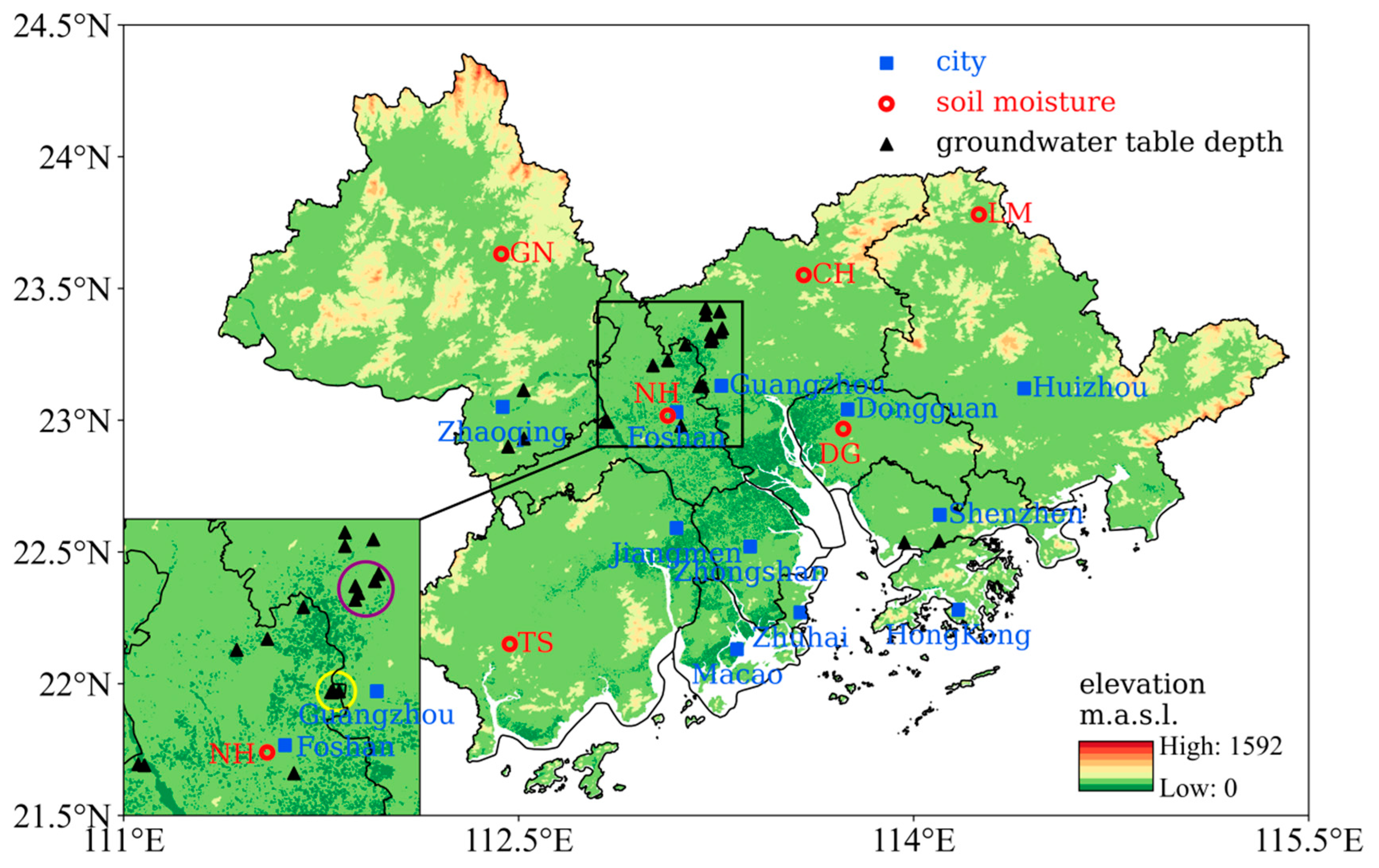
Figure 1. Map of the Guangdong–Hong Kong–Macao Greater Bay Area and station locations. Red dots indicate the six in situ observation stations of soil moisture observations, blue square dots indicate the main cities, and black triangular dots indicate the 26 water wells of groundwater table depth. The yellow circle contains five water wells of groundwater table depth, and the purple circle contains seven water wells of groundwater table depth.
Sustainability 15 10776 g001
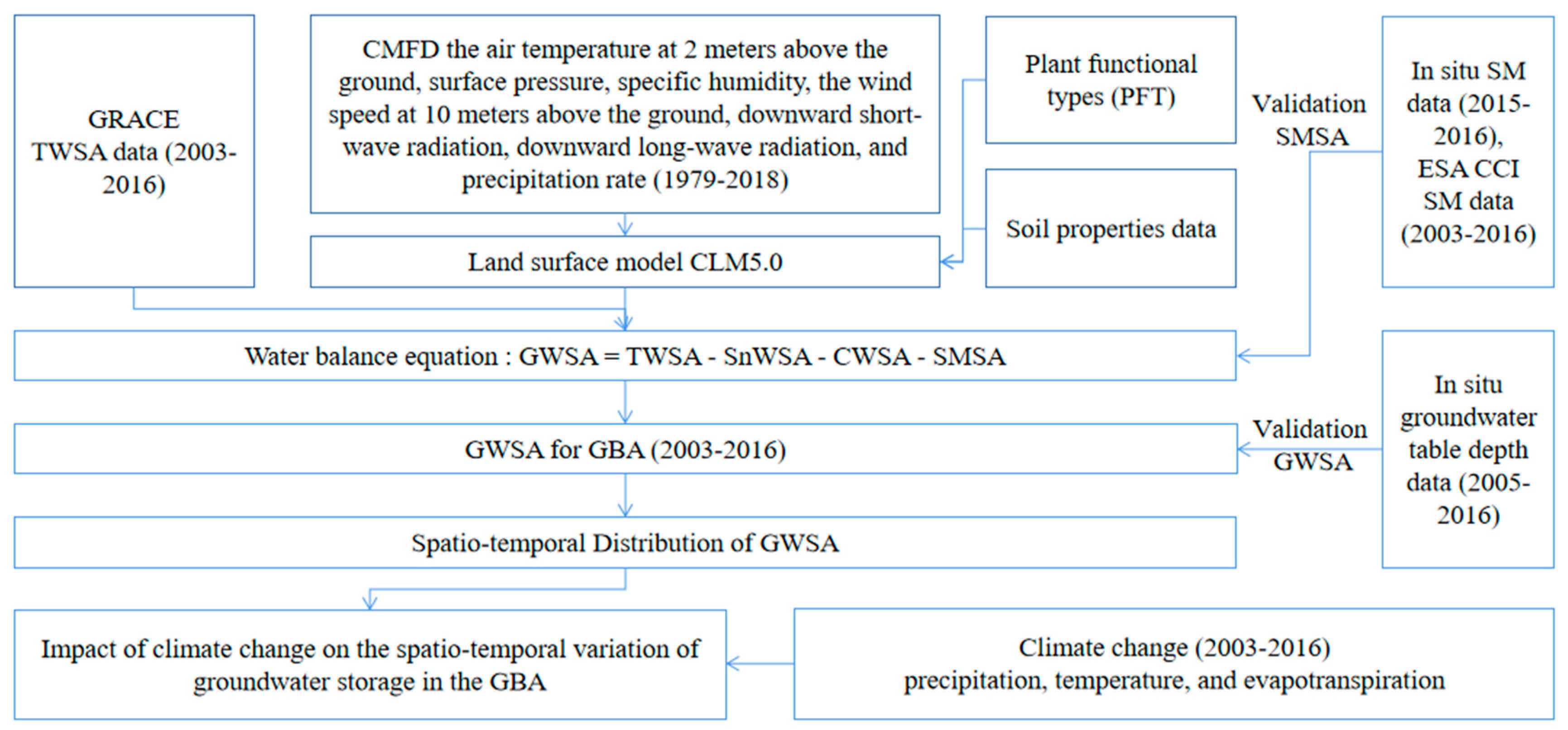
Figure 2. Technical flowchart for estimating the GWSA of the GBA (2003–2016) using GRACE and CLM5.0. SM and GWSA were also validated, and the impact of climate change on the spatio-temporal variation in GWSA in the GBA was quantitatively assessed.
Sustainability 15 10776 g002
Figure 3. (a) Spatial distribution, (b) spatial distribution of the linear trend, and the (c) time series of groundwater storage anomaly in the Guangdong–Hong Kong–Macao Greater Bay Area in the period 2003–2016. The shaded areas represent grids with statistically significant trends, * p < 0.05.
Sustainability 15 10776 g003
Figure 4. (a) Annual time series of the simulated (red line) and observational (blue line) soil moisture (SM) over the period extending from September 2015 to December 2016. (b) Annual time series of the simulated (red line) and ESA CCI (blue line) SM over the period 2003–2016, * p < 0.05.
Sustainability 15 10776 g004
Figure 5. Spatial distribution of the climatologic states in the period 2003–2016 for (a) the simulated soil moisture (SM) via CLM5.0 and (b) the SM of the European Space Agency’s Climate Change Initiative (ESA CCI). (c,d) Pearson’s correlation coefficient (R) and root mean square error (RMSE) for CLM5.0 and ESA CCI, respectively. The blank areas exist due to missing ESA CCI data.
Sustainability 15 10776 g005
Figure 6. Comparison between annual time series of the calculated groundwater storage anomaly (red line, left) and the observed groundwater level anomaly (blue line, right) from 2005 to 2016. The red line represents the average values of the observations, and the blue line represents the average values of estimated GWSA at the corresponding grid cells for each site.
Sustainability 15 10776 g006
Figure 7. Monthly time series of (a) precipitation, (b) temperature, and (c) evapotranspiration in the GBA from 2003 to 2016.
Sustainability 15 10776 g007
Figure 8. Spatial distribution of precipitation, temperature, and evapotranspiration ((a,c,e), respectively, averaged between 2003 and 2016, and the spatial distribution of linear trends of precipitation, temperature, and evapotranspiration from 2003 to 2016 ((b,d,f), respectively).
Sustainability 15 10776 g008
Figure 9. Contribution of (a) precipitation, (b) temperature, and (c) evapotranspiration to groundwater storage anomaly (GWSA) in the Guangdong–Hong Kong–Macao Greater Bay Area. (d) Spatial distribution of the main controlling factors affecting GWSA; a, b, and c represent precipitation, temperature, and evapotranspiration, respectively.
Sustainability 15 10776 g009
Table 1. Statistical results (mean squared error (MSE), Pearson’s correlation coefficient (R), and Taylor’s skill score (TSS)) of the CLM5.0 SM simulated against ESA CCI (regional averaged values) and in situ (site averaged values) SM data.
Test StatisticCLM5.0 with ESACCI DataCLM5.0 with In Situ SM Data
MSE0.0020.01
R0.810.89
TSS0.580.29
Disclaimer/Publisher’s Note: The statements, opinions and data contained in all publications are solely those of the individual author(s) and contributor(s) and not of MDPI and/or the editor(s). MDPI and/or the editor(s) disclaim responsibility for any injury to people or property resulting from any ideas, methods, instructions or products referred to in the content.