Abstract
Reducing car dependence is the key to achieving the goal of green and sustainable development. Compared with the existing studies, which mainly focus on administrative areas, this study takes residential areas as the research unit. Four spatial regression models were used to investigate the effect on car dependence of six factors of the built environment (land use mix, population density, jobs–housing balance, bus stop density, metro station density, and road network density). Various test results show that the geography-weighted regression (GWR) model has more substantial explanatory power and that the estimated coefficients of built environment characteristics vary positively or negatively in diverse residential communities. The findings demonstrate that the impact of built environment characteristics on car dependence is significantly spatially heterogeneous. These results are conducive to better comprehending how built environment factors affect car dependence and help establish policies and strategies to promote sustainable transportation.
1. Introduction
Car dependence contributes to various global issues, such as air pollution and traffic congestion, which have led to an upsurge in research about the connection between the built environment and car dependence [1,2,3]. Chinese cities are showing the characteristics of sprawling development. The rapid expansion of the urban scale and the ever-increasing travel demand further increase residents’ dependence on cars [4]. Technological innovation, such as the rapid growth of electric vehicles, cannot solve urban problems or even generate unprecedented electricity demand [5,6]. To alleviate a series of problems caused by residents’ excessive reliance on cars, many scholars have explored the behavioral characteristics and reasons for reducing residents’ dependence on automobile travel by optimizing the built environment [7].
Planners and managers are still confused about improving the proportion of green travel by optimizing the built environment, although researchers have achieved many results. The built environment determines the spatial distribution of residents’ daily activities and affects travel distribution and mode selection. Research has shown that compact development models that enhance land use mix [8] and population density [9] can reduce car use. However, some scholars have come up with conflicting views. Yin and Sun pointed out in their study of 48 cities in China that an increasing land mix stimulated the demand for car travel and led to an increase in car ownership and dependence on car travel. However, the cost of travel was falling [10]. These conclusions make managers puzzled about whether the built environment’s impact on residents’ use of cars is fluctuating. Is there spatial heterogeneity in the suburbs and urban centers in urban construction? What priorities can measures achieve to more significant results with limited investment?
The phenomenon of population concentration and urban expansion in cities is widespread worldwide, and the number of megacities is also increasing. It is worth discussing whether the built environment’s impact on travel behavior in suburban areas has changed compared with the central urban area. This requires breaking through the research approach that takes the city as the object and exploring the phenomena and laws at the community scale or even smaller research unit scale [11,12].
Therefore, this paper took residential areas as the object and analyzed the impact of the built environment around residential areas on residents’ car use. A relative car-dependent quantitative calculation index was proposed using the location entropy model to replace subjective quantitative methods such as travel distance and sharing rate. Geographically weighted regression (GWR) is a method of fitting different regression equations based on spatial location that was used to capture the heterogeneity and complexity of the impact of built-up environments around residential areas on car use. R2, log likelihood value, Akachi information criterion (AIC), and other indicators all showed that GWR is superior to linear regression models, the spatial error model, and the spatial Dubin model.
This study contributes to existing studies in two aspects. Firstly, the location entropy model, the ratio of ratio, is used to quantify the degree of car dependence in residential areas. This model is mainly used to analyze the spatial distribution of elements in a specific region and does not need to set a threshold subjectively. Secondly, the GWR model, a locally variable parameter model, is used to analyze the relationship between the built environment around residential areas and the dependence on cars. The model reveals the spatial heterogeneity of the built environment’s impact on the use of vehicles. To some extent, the research results and conclusions answer why the existing research cannot reach a unified view on a particular element. This research enables planners to better understand how the building environment affects the use of cars by residents.
This paper is structured as follows: Section 2 briefly reviews existing studies on the built environment and car dependence; Section 3 and Section 4 introduce the research data and methods, respectively; Section 5 presents a case study; Section 6 is an in-depth discussion of the research results; and Section 7 concludes the research.
2. Literature Review
Research on the impact of the urban built environment on car travel behavior is mainly reflected in urban design and transportation systems. The urban design includes land use mix, population density, etc. The transportation system includes public transportation and road network density [12].
The relationship between job and residence is one of the first elements to be studied. Zhou et al. (2014) analyzed the relationship between job and residence balance and commuting efficiency in Xi’an, China. The research results show that the ratio of jobs to residences in quantity and space significantly impacts commuting efficiency [13]. Ta et al. (2017) also confirmed that government intervention could help reduce commute time. They suggested that the government should consider promoting the mixed use of land and urban planning, focusing on the balance of occupation and residence [8]. Li and Zhao (2017) showed that mixed land use and living closer to shopping malls, restaurants, and other areas could reduce the willingness to buy cars [14]. However, Yin and Sun (2018) reached the opposite conclusion. They pointed out that land mixing will stimulate the demand for car travel and increase car ownership and dependence on car travel, although the mixed use of land may reduce travel costs [10].
The impact of public transport on car travel is the focus of scholars’ research. Milakis (2015) believed that people living in communities with high population and work density near the subway station tend to travel short distances and prefer more environmentally friendly transportation [15]. Ma (2015) showed that community residents with high work density, close proximity to the sub-center of the city, vital subway accessibility, and mixed land use have short travel distances. Commuting travel differentiation among community residents is higher than non-commuting travel [16]. A Choi (2018) study in Calgary, Canada, found that light rail is the key to reducing car travel. In addition, when living in a place far away from the city center, the number of trips will increase significantly, and the city center has gathered more than half of the city’s jobs, which means that the sub-central area needs to be established in the whole town [17]. Yang et al. (2021) found that higher urban public transport coverage can reduce the number of driving trips by citizens, but it cannot reduce car ownership. This study shows that the built environment has a more significant impact on travel mode choice than the number of cars [18]. Some studies have shown that traditional public transportation’s service quality and attractiveness are declining compared with other modes of transportation, such as shared transportation, bicycles, electric vehicles, etc. The impact of traditional public transit on reducing car travel is weakening [19].
The impact of the built environment on automobile dependence is far from consensus. In terms of research methods, the existing research mainly uses a generalized linear model [20], a structural equation model [16], a Bayesian model, a machine learning model, a spatial econometric model, and other methods to model the impact of the built environment on residents’ car ownership and user behavior. These studies usually draw a broad conclusion on the relationship between the built environment and car dependence at the level of cities or administrative regions. The judgment on the impact of built environments, such as land use mixing and conventional public transportation, on residents’ car use is divergent.
The interdisciplinary methods, such as the local variable parameter model in geography, provide new ideas for this study. The geographically weighted regression (GWR) is the most typical local variable parameter model used to capture spatial heterogeneity and reveal microscopic differences. The GWR model has been used to analyze the spatial and temporal distribution of taxi travel [21], active travel [22], and bus travel [23] and the relationship between potential impact variables. These research results prove that the GWR model has better explanatory power than linear regression and other methods.
3. Data
3.1. Resident Travel Data
This research utilized the travel data of residents from the 2019 survey of traffic behavior and willingness of Shenzhen residents, which the Shenzhen Transportation Bureau and Shenzhen Urban Transport Planning Center Co. jointly organized. The resident study was stratified according to the number of administrative districts, streets, and community management and service populations. A total of about 11,000 households and 20,000 interviewees were effectively surveyed. Figure 1 shows the spatial location of the surveyed households. The questionnaire is divided into three parts: family characteristics, personal characteristics, and a travel chain survey. The travel chain data includes the origin and destination of the respondents, the distance, time, and mode of transportation of each journey.
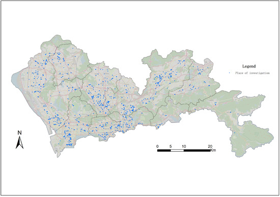
Figure 1.
Location distribution of sampling survey.
Definition 1.
The car dependence index (CDI) was used to define the degree of dependence of each residential area on car use. Location entropy, a method used to reflect the concentration of factors, was used to calculate CDI. A significant advantage of this method is that it can spatially calculate the aggregation degree of some aspects without considering the number of other elements [24]. For each residential area, the CDI is defined as:
where is the car travel distance of all interviewees in the residential area i, is the car travel distance of all investigators, is the travel distance of all interviewees in the residential area i, and is the travel distance of all investigators.
3.2. Built Environment Data
To study the impact of the built-up environment around each residential area on the use of residents’ cars, it is necessary to determine the spatial scope of residents’ activities. The travel distance of residents is different, so it is required to calculate the range of activities in each residential area [25].
Definition 2.
The travel radius of residents (TRR) is used to measure the spatial range of the main activity trajectories of residents. The radius of the gyration method was used to calculate TRR [26]. TRR is used to construct the catchment area of each residential area and calculate the built-up environmental elements within the catchment area. For each residential area, the TRR is defined as:
where refers to the longest travel distance of the kth resident in the residential area i and is the number of individual trajectories.
Definition 3.
It is generally accepted internationally that the built-up environment consists of three aspects: land use, urban design, and transportation systems, and it also includes human activity patterns in the physical environment [1]. The architectural and environmental factors that may affect residents’ travel are selected as follows:
3.2.1. F1: Land Use Mix
Existing studies usually use the concept of entropy to reflect land use [24], and the calculation formula is:
where is the land use mixing degree within the catchment area of residential i, is the ratio of the number of type j POIs in residential i to the number of all types of POIs, and is the number of POI types.
3.2.2. F2: Population Density
This research utilized Tencent user data in 2019 obtained from the Urban Data Party company. This study’s resolution is approximately 1 km × 1 km (0.01 × 0.01 degrees). According to Tencent’s official data (https://bigdata.qq.com), in 2020, active accounts exceeded 800 million, more than half of China’s total population. In many big cities in China, Tencent users account for more than 90% of the population. Therefore, many Chinese scholars use these data to analyze the spatial distribution of China’s population density [25].
3.2.3. F3: Jobs–Housing Balance
Defining the jobs–dwelling balance as the distribution of employment relative to the distribution of housing within a given geographical area. Jobs–dwelling balance is an essential factor affecting residents’ travel [13]. The jobs–housing balance data used in this study are from the Shenzhen Municipal Bureau of Statistics, including the 1 km × 1 km (0.01 × 0.01 degrees) grid population and jobs.
3.2.4. F4–F5: Bus Stop Density/Metro Station Density
The public transport system affects the choice of residents’ travel modes. Bus stop density and Metro station density are generally considered to measure the convenience of the public transport system [27]. The bus stop density data used in this study is from the Shenzhen Transportation Bureau. The Metro station density data used in this study is from the Shenzhen Transportation Bureau.
3.2.5. F6: Road Network Density
Road network density, or road length per km2 within the TRR, is another major factor affecting residents’ travel choices [28]. The road network data used in this study comes from the OSM website. The road types include expressways, main roads, secondary roads, and branch roads.
The variance expansion factor (VIF) is introduced to ensure no multicollinearity of variables.
4. Methods
4.1. Spatial Autocorrelation Method
Moran’s I index was used to evaluate the spatial distribution characteristics of the travel emission sources. It is an indicator of spatial correlation. Moran’s statistics are expressed as follows:
where represents the deviation of the attribute of element i from its average value, represents the spatial weight between part i and component j, and n is the sum of the elements.
The statistical z-score is calculated as follows:
where is the weighted mean of the total emissions and the standard deviation.
|Z| > 2.58 is regarded as statistically significant, and the confidence level of statistical significance is set to 99% (less than 0.01) [24].
ArcGIS software was used to calculate Moran’s I and the verification indicators. The Moran’s I value ranges from −1 to 1. When the value is close to 1, it indicates a positive correlation; when it equals 0, it means no correlation.
4.2. Spatial Metrology Model
Econometric models are widely used to describe the quantitative characteristics of natural economic systems and to reveal the impact of quantitative system changes. With the introduction of spatial dependence and spatial heterogeneity into regression models, spatial econometric models are widely used to study the effects of spatiotemporal data. The spatial error model (SEM) considers spatial dependence, which is measured through the spatial autocorrelation setting of error terms. The SEM model is constructed as follows:
where represents the car dependence index of the residential area i; represents the estimated parameters; represents the p-th independent variable of the residential area i; represents the number of independent variables; represents the coefficient of the spatial correlation error term; represents the spatial weight, which is determined by calculating the spatial distance according to the longitude and latitude coordinates of residence communities i and j; is the longitude and latitude coordinate of residential area j; is the error term and follows the normal distribution.
Considering the spatial correlation of urban spatial dependent variables and the spatial correlation of independent variables, the spatial Dubin model (SDM) is constructed to add corresponding constraints to the spatial lag and error models. The SDM model is built as follows:
where represents the coefficient of the spatial lag term , and and are estimated parameters.
The regression coefficient of the spatial econometric model is not affected by the spatial location of the sample. The model reflects the explanation of spatial correlation in the lag term, or error. This result causes the model to ignore the spatial heterogeneity of the data and leads to inaccurate estimation results. The GWR model extends the generalized linear regression model, which can overcome this problem. The GWR model allows the regression coefficient of the variable to change with its position in space. In addition, the regression results of the GWR model have smaller fitting residuals, and the explanatory variables are less spatially dependent. It is expressed as follows:
where is a dimensional interpretation variable, is a dimensional interpretation variable matrix, is the regression coefficient of factor k at the regression point, represents the coordinates at the ith observation point, and is the random error term of the independent distribution.
The Gaussian kernel was chosen to calculate the spatial weighting coefficient. Then we selected the optimal bandwidth by the cross-validation method, and the mode was set to have the same window-width parameter at each quantifier for comparison and calculation [29].
The effect of model fitting is comprehensively evaluated by multiple indicators, including R2, log-likelihood value, Akachi information criterion (AIC), and Moran’s I index of residual.
5. Results
Shenzhen is a megacity in the southeast coastal area of China. Shenzhen’s GDP exceeded 3 trillion RMB (around 475 billion USD) and ranked third of the 35 major cities across China in 2021. Shenzhen, one of the fastest-growing cities in China, is an excellent case study for studying automobile dependence in China. The study area includes all nine municipal districts of Shenzhen.
5.1. Spatial Analysis of the Travel Distance
Table 1 lists the calculation results of the spatial autocorrelation of the car travel distance. The Z-scores exceed 2.58, indicating the statistical significance of the data. The p-value was less than 0.01, demonstrating that car dependence data had a positive spatial autocorrelation (Moran’s I > 0). Figure 2 shows the spatial distribution of the travel distance of residents’ cars. From red to green, the travel distance of residents decreases in turn.

Table 1.
Spatial correlation analysis results.
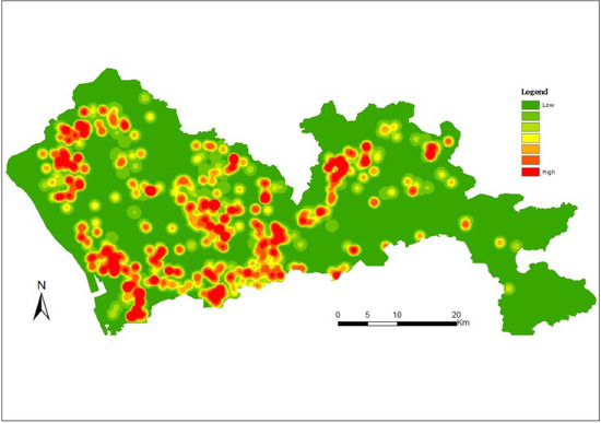
Figure 2.
Spatial distribution of travel distances for residents’ cars. Red and green values decrease gradually.
5.2. Regression Analysis of the Travel Distance
Table 2 lists the six factors’ VIFs as less than 10, indicating no multicollinearity between the six variables.
Table 2.
Six elements of VIF.
Table 3 lists the four regression model-fitting effect evaluation indicators. The interpretation abilities of OLS, SEM, and SDM were between 40% and 46%. Moran’s I index of AIC and residuals of SEM and SDM models is better than that of OLS models, proving that taking spatial dependence as a variable can better describe the spatial effect of the built environment on car use.
Table 3.
Evaluation index of regression model fitting effect.
The GWR model-fitting effect is significantly better than SEM and SDM. The adjusted R2 of the GWR is about 0.597, which is higher than the SEM and SDM models. The Moran’s I value of the GWR residual decreased to 0.001, indicating that the spatial autocorrelation of the residuals had significantly weakened or disappeared in the GWR models [27]. The GWR model had a smaller value of the AIC, meaning it was a better-fitting regression model [30]. Considering the interpretation ability and complexity of the model, as well as the effect of dealing with the impact of spatial complexity, GWR has the best fitting effect, followed by SLM and SEM.
Table 4 shows the regression model’s calculation results, and each influencing factor’s significant consequences are consistent. Land use and rail transit station density significantly negatively affected car dependence at the 5% level (p < 0.05). Road network density significantly positively affected car dependence at the 5% level (p < 0.05). The population density greatly affected car dependence at the 1% level (p < 0.01). In contrast, the jobs–housing balance and the number of regular bus stops had no significant impact on residents’ car travel.
Table 4.
Regression model parameter estimation results.
Table 5 shows the coefficient range (maximum, minimum, and median) of the influence of the four factors calculated by the GWR model on car dependence. From the average coefficients of built environments in Table 5, land use mix, population density, and metro station density adversely affect residents’ reliance on cars. However, the maximum and minimum impact coefficients of the land use mix are 1.11 and −3.34, respectively, indicating that the land use mix positively affects the dependence on cars in some communities. In contrast, other areas may have a negative effect. The maximum and minimum impact coefficients of population density are −7.13 and 0.37, respectively. The maximum and minimum impact coefficients of metro station density are −3.75 and 1.81, respectively. Road network density’s top and minimum impact coefficients are −0.35 and 0.58, respectively.
Table 5.
The varying coefficients of the GWR model.
Figure 3 shows the spatial distribution of the estimated coefficients. The red residential area indicates that the estimated benefits of the built environment are positive ( > 0). In contrast, the green residential area suggests that the estimated benefits of the built environment are negative ( < 0). As depicted in Figure 3a, when residence communities are from west to east, the estimated coefficient of the land use mix changes from positive to negative, which indicates that the correlation between land use mix and resident car dependence varies from positive to negative. Figure 3b shows that the population density in the central region promotes the support of residents for cars, while the other areas have the opposite effect. Figure 3c demonstrates that, in addition to the suburbs, the improvement of metro station density can effectively reduce the use of cars by residents. Figure 3d shows that increasing road network density will lead to more dependence on vehicles in areas other than the urban center and Guangming New Area.
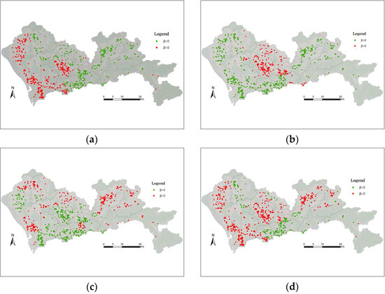
Figure 3.
Spatial distribution of estimated coefficients. The red color indicates > 0 and the green indicates < 0. (a) F1 (land use mix). (b) F2 (population density). (c) F5 (metro station density). (d) F6 (road network density).
Figure 4 shows the spatial distribution of the estimated coefficient of the built environment’s inhibition of car dependence, where green to red indicates a more significant impact. The influence of land use mixing degree on vehicle use shows a multi-gradient changing trend. The result of road network density on reducing automobile dependence shows a decreasing trend from the central area to the suburbs. The effect of population density on reducing automobile dependence shows a decreasing trend from the geographical center to other regions. The influence of the number of subway stations on reducing automobile dependence also shows a multi-gradient trend.
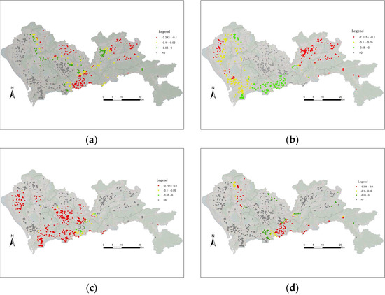
Figure 4.
The spatial distribution of the estimated coefficients for restraining car dependence. Red and green values decrease gradually. (a) F1 (land use mix). (b) F2 (population density). (c) F5 (metro station density). (d) F6 (road network density).
6. Discussion
Our results provide new insights for improving the built environment, reducing car dependence, and developing sustainable transportation.
The estimated coefficient of the built environment shows significant spatial heterogeneity within the residence communities studied, suggesting that the influence of built environment factors on car dependence varies by geographical location. From the average coefficients of built environments, land use mix, population density, and metro station density negatively affect residents’ reliance on cars. In the western region of Shenzhen, the land use mix may positively affect residents’ automobile dependence. In the central area of Shenzhen, the increase in population density may encourage residents to use more cars to travel. This result explains why some studies believe that land use mix and population density can inhibit vehicle use [8,14], while others put forward the opposite view [17,18].
The case of Shenzhen demonstrates the changes in the impact coefficient, and planners can prioritize building environments that suppress the impact coefficient of car use. Some community-scale studies on residents’ travel also provide similar perspectives [28]. For residents living in Futian Central District, the main factors that encourage them to reduce their use of cars are land use mix and road network density. Increasing population density and the number of rail transit stations will not significantly increase the proportion of green travel. However, for residents in Baoan District, increasing the building density (population density) and the number of rail transit stations will play a key role in reducing the use of cars. We believe differentiated strategies are essential, especially when financial support is limited.
Our research also found that bus stop density does not significantly impact residents’ car use. Some managers from public transportation companies are also confused. Survey data shows that in the structure of residents’ commuting modes, the proportion of non-motorized and motorized travel is about 47% and 53%, respectively. The ratio of public transportation (regular buses, subways, and taxis) is about 29.5%, higher than the 23.0% of cars. Compared with 2016, the average commuting distance has increased from 5.6 km to 7.0 km, and the average motorized commuting distance has increased from 8.6 km to 11.3 km. The travel time has increased from 21 min to 31 min. Among them, the average public transportation travel time is 47 min, and that of private cars is 36 min. Residents’ main demands are building a subway network, reducing subway congestion, improving bus operation speed, and increasing bus departure frequency. Some new ideas include improving bus punctuality, comfort, safety, and convenience to enhance passenger satisfaction and loyalty. Developing customized public transport and replacing small vehicles to increase direct routes may be a new way to encourage people to choose public transport. In the practice of Futian Central District in Shenzhen, stabilizing measures such as dynamic speed limits based on road conditions are considered to improve the safety of non-motorized traffic.
In this paper, the effects of factors such as family attributes, personal attributes, and other elements on vehicle dependence were not considered owing to data limitations, which may impact the fitness of the modeling results. Our case has only been demonstrated using data from Shenzhen, and it is currently impossible to obtain large-scale travel survey data for other trips. This is the weakness of this study, and further research is needed in the future. The GWR model can reflect the non-stationary spatial relationship between the dependent and independent variables. Its advantages in analyzing the heterogeneity and complexity of spatial data for various urban transportation modes have been proven in other studies [21,23]. This article provides a new approach to studying the built-up environment and car dependence at the residential area scale.
7. Conclusions
There have been many disagreements in the study of the impact of urban-scale built-up environments on residents’ dependence on cars, causing confusion among planners and managers on how to improve the proportion of green travel by optimizing the built environment. This study uses the travel survey data of Shenzhen residents to answer the following questions: Is there spatial heterogeneity between suburbs and urban centers in urban construction? What priority measures can achieve more significant results with limited investment?
All four model validation indicators indicate that the GWR model has better fitting performance and explanatory power. From the average coefficients of built environments, land use mix, population density, and metro station density negatively affect residents’ reliance on cars. The estimated coefficient of the built environment shows significant spatial heterogeneity within the residence communities studied, suggesting that the influence of built environment factors on car dependence varies by geographical location. Planners can prioritize building environments that suppress the impact coefficient of car use, and differentiation strategies are essential, especially when financial support is limited. The density of bus stops has no significant impact on residents’ car use. Improving the punctuality, comfort, safety, and convenience of buses rather than simply increasing the density of bus stops is beneficial for attracting passengers to choose buses instead of cars.
However, the findings may vary among different cities. More case studies are needed to test whether the results are generalizable to other cities. Subsequent studies will consider improving input parameters, such as public transport accessibility, instead of bus station density. Improving the calculation model, such as the Gradient Boosting Decision Tree, will also be the main object of the author’s subsequent research.
Author Contributions
Conceptualization, J.J. and J.W.; methodology, M.S.; software, J.J.; validation, J.W.; formal analysis, J.J.; investigation, J.J.; resources, J.J.; data curation, J.J.; writing—original draft preparation, J.J.; writing—review and editing, J.W. and S.C.; visualization, J.W.; supervision, J.W.; project administration, X.Z.; funding acquisition, X.Z. All authors have read and agreed to the published version of the manuscript.
Funding
This research was supported by the National Natural Science Foundation of China (grant No. 71734004).
Institutional Review Board Statement
Not applicable.
Informed Consent Statement
Not applicable.
Data Availability Statement
Not applicable.
Acknowledgments
The author would like to thank the editors and reviewers for their valuable comments and suggestions, which enabled us to improve the quality of the paper.
Conflicts of Interest
The authors declare no conflict of interest.
References
- Wang, X.; Yin, C.; Zhang, J.; Shao, C.; Wang, S. Nonlinear effects of residential and workplace built environment on car dependence. J. Transp. Geogr. 2021, 96, 103207. [Google Scholar] [CrossRef]
- Zhang, W.; Zhang, M. Incorporating land use and pricing policies for reducing car dependence: Analytical framework and empirical evidence. Urban Stud. 2017, 55, 3012–3033. [Google Scholar] [CrossRef]
- Zegras, C. The Built Environment and Motor Vehicle Ownership and Use: Evidence from Santiago de Chile. Urban Stud. 2010, 47, 1793–1817. [Google Scholar] [CrossRef]
- Yin, C.; Shao, C.; Wang, X. Built Environment and Parking Availability: Impacts on Car Ownership and Use. Sustainability 2018, 10, 2285. [Google Scholar] [CrossRef]
- Li, W.; Yang, M.; Long, R.; He, Z.; Zhang, L.; Chen, F. Assessment of greenhouse gasses and air pollutant emissions embodied in cross-province electricity trade in China. Resour. Conserv. Recycl. 2021, 171, 105623. [Google Scholar] [CrossRef]
- Li, W.; Long, R.; Zhang, L.; Cheng, X.; He, Z.; Chen, F. How the uptake of electric vehicles in China leads to emissions transfer: An Analysis from the perspective of inter-provincial electricity trading. Sustain. Prod. Consum. 2021, 28, 1006–1017. [Google Scholar] [CrossRef]
- Zhao, P.; Bai, Y. The gap between and determinants of growth in car ownership in urban and rural areas of China: A longitudinal data case study. J. Transp. Geogr. 2019, 79, 102487. [Google Scholar] [CrossRef]
- Ta, N.; Chai, Y.; Zhang, Y.; Sun, D. Understanding job-housing relationship and commuting pattern in Chinese cities: Past, present and future. Transp. Res. Part D Transp. Environ. 2017, 52, 562–573. [Google Scholar] [CrossRef]
- Thao, V.T.; Ohnmacht, T. The impact of the built environment on travel behavior: The Swiss experience based on two National Travel Surveys. Res. Transp. Bus. Manag. 2019, 36, 100386. [Google Scholar] [CrossRef]
- Yin, C.; Sun, B. Disentangling the effects of the built environment on car ownership: A multi-level analysis of Chinese cities. Cities 2018, 74, 188–195. [Google Scholar] [CrossRef]
- Zhang, W.; Zhao, Y.; Cao, X.; Lu, D.; Chai, Y. Nonlinear effect of accessibility on car ownership in Beijing: Pedestrian-scale neighborhood planning. Transp. Res. Part D Transp. Environ. 2020, 86, 102445. [Google Scholar] [CrossRef]
- Hou, Y.; Moogoor, A.; Dieterich, A.; Song, S.; Yuen, B. Exploring built environment correlates of older adults’ walking travel from lifelogging images. Transp. Res. Part D Transp. Environ. 2021, 96, 102850. [Google Scholar] [CrossRef]
- Jiangping, Z.; Chun, Z.; Xiaojian, C.; Wei, H.; Peng, Y. Has the legacy of Danwei persisted in transformations? the jobs-housing balance and commuting efficiency in Xi’an. J. Transp. Geogr. 2014, 40, 64–76. [Google Scholar] [CrossRef]
- Li, S.; Zhao, P. Exploring car ownership and car use in neighborhoods near metro stations in Beijing: Does the neighborhood built environment matter? Transp. Res. Part D Transp. Environ. 2017, 56, 1–17. [Google Scholar] [CrossRef]
- Milakis, D.; Cervero, R.; Van Wee, B. Stay local or go regional? Urban form effects on vehicle use at different spatial scales: A theoretical concept and its application to the San Francisco Bay Area. J. Transp. Land Use 2015, 8, 59–86. [Google Scholar] [CrossRef]
- Ma, J.; Liu, Z.; Chai, Y. The impact of urban form on CO2 emission from work and non-work trips: The case of Beijing, China. Habitat Int. 2015, 47, 1–10. [Google Scholar] [CrossRef]
- Choi, K. The influence of the built environment on household vehicle travel by the urban typology in Calgary, Canada. Cities 2018, 75, 101–110. [Google Scholar] [CrossRef]
- Yang, L.; Ding, C.; Ju, Y.; Yu, B. Driving as a commuting travel mode choice of car owners in urban China: Roles of the built environment. Cities 2021, 112, 103114. [Google Scholar] [CrossRef]
- Liao, Y.; Gil, J.; Pereira, R.H.M.; Yeh, S.; Verendel, V. Disparities in travel times between car and transit: Spatiotemporal patterns in cities. Sci. Rep. 2020, 10, 4056. [Google Scholar] [CrossRef]
- Sprumont, F.; Scheffer, A.; Caruso, G.; Cornelis, E.; Viti, F. Quantifying the Relation between Activity Pattern Complexity and Car Use Using a Partial Least Square Structural Equation Model. Sustainability 2022, 14, 12101. [Google Scholar] [CrossRef]
- Tang, J.J.; Gao, F.; Liu, F.; Zhang, W.H.; Qi, Y. Understanding Spatio-Temporal Characteristics of Urban Travel Demand Based on the Combination of GWR and GLM. Sustainability 2019, 11, 5525. [Google Scholar] [CrossRef]
- Rybarczyk, G. Toward a spatial understanding of active transportation potential among a university population. Int. J. Sustain. Transp. 2018, 12, 625–636. [Google Scholar] [CrossRef]
- He, Y.X.; Zhao, Y.; Tsui, K.L. Geographically Modeling and Understanding Factors Influencing Transit Ridership: An Empirical Study of Shenzhen Metro. Appl. Sci. 2019, 9, 4217. [Google Scholar] [CrossRef]
- Sun, M.; Xue, C.; Cheng, Y.; Zhao, L.; Long, Z. Analyzing Spatiotemporal Daily Travel Source Carbon Emissions Based on Taxi Trajectory Data. IEEE Access 2021, 9, 107012–107023. [Google Scholar] [CrossRef]
- Sun, M.; Gao, C.; Xue, C.; Zhang, S.; Li, C. A Data-Driven Method for Measuring Accessibility to Healthcare Using the Spatial Interpolation Model. IEEE Access 2021, 9, 64972–64982. [Google Scholar] [CrossRef]
- Rhee, I.; Shin, M.; Hong, S.; Lee, K.; Kim, S.J.; Chong, S. On the Levy-Walk Nature of Human Mobility. IEEE/ACM Trans. Netw. 2011, 19, 630–643. [Google Scholar] [CrossRef]
- Yang, W.Y.; Chen, B.Y.; Cao, X.S.; Li, T.; Li, P. The spatial characteristics and influencing factors of modal accessibility gaps: A case study for Guangzhou, China. J. Transp. Geogr. 2017, 60, 21–32. [Google Scholar] [CrossRef]
- Feng, R.; Feng, Q.; Jing, Z.; Zhang, M.; Yao, B. Association of the built environment with motor vehicle emissions in small cities. Transp. Res. Part D Transp. Environ. 2022, 107, 103313. [Google Scholar] [CrossRef]
- Xia, C.; Xiang, M.; Fang, K.; Li, Y.; Ye, Y.; Shi, Z.; Liu, J. Spatial-temporal distribution of carbon emissions by daily travel and its response to urban form: A case study of Hangzhou, China. J. Clean. Prod. 2020, 257, 120797. [Google Scholar] [CrossRef]
- Kaya, E.; Agca, M.; Adiguzel, F.; Cetin, M. Spatial data analysis with R programming for environment. Hum. Ecol. Risk Assess. Int. J. 2019, 25, 1521–1530. [Google Scholar] [CrossRef]
Disclaimer/Publisher’s Note: The statements, opinions and data contained in all publications are solely those of the individual author(s) and contributor(s) and not of MDPI and/or the editor(s). MDPI and/or the editor(s) disclaim responsibility for any injury to people or property resulting from any ideas, methods, instructions or products referred to in the content. |
© 2023 by the authors. Licensee MDPI, Basel, Switzerland. This article is an open access article distributed under the terms and conditions of the Creative Commons Attribution (CC BY) license (https://creativecommons.org/licenses/by/4.0/).