Article

Life Insurance Prediction and Its Sustainability Using Machine Learning Approach

by
Siti Nurasyikin Shamsuddin
1,2,*,
Noriszura Ismail
1 and
R. Nur-Firyal
1,*
1
Department of Mathematical Sciences, Faculty of Science & Technology, Universiti Kebangsaan Malaysia, Bangi 43600, Malaysia
2
Mathematical Sciences Studies, College of Computing, Informatics and Media, Universiti Teknologi MARA Cawangan Negeri Sembilan, Kampus Seremban, Seremban 70300, Malaysia
*
Authors to whom correspondence should be addressed.
Sustainability 2023, 15(13), 10737; https://doi.org/10.3390/su151310737
Submission received: 26 May 2023 / Revised: 6 July 2023 / Accepted: 6 July 2023 / Published: 7 July 2023

Abstract

:
Owning life insurance coverage that is not enough to pay for the expenses is called underinsurance, and it has been found to have a significant influence on the sustainability and financial health of families. However, insurance companies need to have a good profile of potential policyholders. Customer profiling has become one of the essential marketing strategies for any sustainable business, such as the insurance market, to identify potential life insurance purchasers. One well-known method of carrying out customer profiling and segmenting is machine learning. Hence, this study aims to provide a helpful framework for predicting potential life insurance policyholders using a data mining approach with different sampling methods and to lead to a transition to sustainable life insurance industry development. Various samplings, such as the Synthetic Minority Over-sampling Technique, Randomly Under-Sampling, and ensemble (bagging and boosting) techniques, are proposed to handle the imbalanced dataset. The result reveals that the decision tree is the best performer according to ROC and, according to balanced accuracy, F1 score, and GM comparison, Naïve Bayes seems to be the best performer. It is also found that ensemble models do not guarantee high performance in this imbalanced dataset. However, the ensembled and sampling method plays a significant role in overcoming the imbalanced problem.

1. Introduction

Life insurance protects beneficiaries if any accidental death or unexpected event happens [1]. However, in countries with well-established social security systems, the demand for life insurance is frequently low [2]. The perception of mortality risk and attitudes toward life insurance plays a vital role in purchasing a life insurance policy. Most households are aware of the monetary risk posed by mortality. This does not, however, lead to the purchase of life insurance, which may affect the sustainability of their finances. A survey by the Swiss Re Institute (2020) [3] claims that households in all of the region’s countries favor other strategies for boosting their financial security over life insurance, such as increasing their income or purchasing medical/critical illness insurance.
Due to the COVID-19 pandemic breakout, life insurance policies have drawn particular attention and interest among the numerous insurance products. The epidemic affects the global economy in both positive and negative ways. A series of surveys with the public were conducted between March and June 2020 in the UK, the US, and Spain. The results revealed that 30% of respondents said COVID-19 had increased their likelihood of considering buying life insurance [4]. However, based on the insurance barometer study conducted by LIMRA and Life Happens in 2021, life insurance ownership in the US decreased marginally in 2021, with only 52% of Americans claiming to have life insurance, a decrease from 54% in 2020 [5].
According to Bank Negara Malaysia (Central Bank of Malaysia), demand for life insurance has increased over the last decade, with per capita life insurance premiums rising 156% from RM 797.00 (USD 176.97)1 in 2010 to RM 1250.00 (USD 277.56) in 2021. Total premiums from new life insurance income rose from RM 7.9 billion to RM 40.75 billion, while new life insurance policies increased from 1.5 million to 17.5 million units. Meanwhile, in 1990, per capita insurance premium expenditure was only RM 92.00 (USD 20.43), while total new premiums (RM 573 million) and the number of new life insurance contracts (498,338) were significantly lower as compared to the period of 2010 to 2021 [6].
Figure 1a shows the number of policies and certificates in force from 2010 to 2021, which showed an increasing trend. However, there was a slight decrease in the number of life insurance policies in force in 2019. Meanwhile, Figure 1b presents the distribution of new sums insured for life insurance, and the sum participated for Takaful Family. In 2020, the distribution of life insurance’s new sums decreased, possibly due to the COVID-19 crisis that affected the nation. The Malaysian life insurance market is still lagging compared to other established global and regional markets, notwithstanding the increase in active policies and premiums mentioned earlier. This is demonstrated by the persistently low insurance density per capita in USD between 2010 and 2021 compared to other Asian nations. Although Malaysia’s insurance intensity climbed by nearly 157% from USD 282.8 in 2010 to USD 444 in 2021—above the world average of USD 382—it still lags behind other developed Asian nations such as Taiwan (USD 3772), Hong Kong (USD 8433), and Singapore (USD 5414). Additionally, in 2021, the Malaysian life insurance penetration rate (the proportion of life insurance premiums to GDP) was estimated to be 3.9%, which is significantly lower than the rates of other developed Asian nations such as Hong Kong (17.3%), Taiwan (11.6%), Singapore (7.5%), and Japan (6.1%) [7].
Based on the above facts, life insurance ownership is an interesting topic, especially in overcoming the low penetration rate problem. Families’ sustainability and financial health were correlated to underinsurance, and one of the methods to overcome underinsurance is to increase the life insurance penetration rate. Hence, various measures must be considered to increase the penetration rate or to attract potential policyholders. One of the initiatives is to classify which one is the potential life insurance purchaser. Data mining techniques are commonly used to discover intriguing patterns in datasets and deliver future helpful information. Different data mining methods work well for classifying customers as potential or non-potential customers.
This study focuses on life insurance ownership in Malaysia, with the status of life insurance purchase as the main observation and Malaysian sociodemographic status as the determinant. Hence, this article uses a data mining approach to classify customers based on their attributes to predict the class label for future customers, whether the potential customers will purchase a life insurance policy or not. This article’s findings will redound to society’s benefit, considering that insurance protection is vital to families’ sustainability and financial health. It may assist insurance companies in better improving their underwriting process in selecting potential purchasers. Besides that, observing the descriptive analysis of the sociodemographic information of the respondents may provide a better overview of the Malaysian target market accordingly, which may increase the country’s life insurance penetration rate. Apart from that, in machine learning and data mining, imbalanced datasets are a constant worry because they make it difficult for machine learning algorithms to efficiently learn minority classes. Hence, this study will also provide insight into the prediction with different sampling and ensemble methods throughout the classification process using data mining techniques because the dataset is imbalanced on a particular class label.

2. Related Work

2.1. The Life Insurance Ownership

For the past decade, a range of demographic factors, including age, gender, marital status, education level, number of dependents, ethnicity, and income, have been the subject of previous studies to determine whether they are significantly related to the decision to purchase (own) life insurance. Few cross-sectional studies have used the decision to buy or not to buy a life insurance policy as a proxy for life insurance demand. Life insurance ownership, the amount of life insurance coverage, the face value, the amount of life insurance premium paid, and the intention to purchase were the primary decision factors employed to estimate the purchasing behavior for life insurance [8]. Meanwhile, age groups, risk aversion, ethnicity, income, education, occupation, and marital status are significant predictors of life insurance in Malaysia. Additionally, to examine the determinants of life insurance demand among married couples in Malaysia, marital status, age, education, ethnicity, and family income are among the significant predictors of life insurance demand [9]. Grabova & Sharku, (2021) found that changes in the urban population, education level, and age dependency ratio statistically impact life insurance density. The penetration rate, however, does not appear to be affected by education level [10].
Several studies have investigated the determinants of life insurance ownership using various methods. A hurdle count-data model is one of the methods used to investigate the factors influencing Malaysians’ life insurance consumption [11]. In 2014, Ref. [12] employed Cragg’s two-part regression model to investigate the sociodemographic factors of household expenditures on life insurance in Malaysia. The study suggested that across ethnic groups, wealth and education levels are correlated with purchase probabilities and the amount of life insurance premiums purchased. However, only within ethnic groups are household size, geographical location, urbanicity, and employment type associated with life insurance demand. Besides that, a Logistic Regression model was used to study the behavior of life insurance purchase decisions among the Indian population. It found that financial circumstances were the most significant determinant of whether a household would purchase insurance or discontinue coverage [13]. Among the demographic factors, family size, gender, and the household head’s education level impacted the likelihood of obtaining or surrendering insurance. Another popular method used by previous researchers is the econometric modeling such as [14,15] with the focus population in Brazil, Russia, India, China, and South Africa (BRICS countries), and the Czech Republic, Hungary, Poland, and Slovak Republic (V4 countries), respectively.
In recent years, machine learning has been proposed as an alternative method in life insurance studies, and it was one of the most trending topics in 2021 [16]. Most of the machine learning research that previous researchers have conducted focuses on life insurance lapse and non-life insurance [17,18].

2.2. Data Mining

There are quite a number of studies with data mining applications in classifying customers, and in this context, insurance customers. Data mining techniques were used by Yan and Xie [19] to study Chinese insurance firms. They suggested classifying data using decision trees and applying data mining to the CRM (Client Relation Management) methodology as well as for risk management. The requirement for insurance firms to operate a sizable data centre or warehouse to store information effectively was also noted.
Next, Thakur and Sing [20] employed a classification approach based on decision trees to create a prediction system based on customer data. They trained data on people who purchased auto insurance online and classified new clients for their interest in online insurance based on the characteristics of the customers. The accuracy and error rate of the classifiers were assessed. The primary goal was to classify customers according to their age, educational level, and the sort of car they drive. As a result, they created a system that offered all the information required for auto insurance online.
Besides that, a study with an imbalanced dataset showed that balancing improved performance significantly. Rahman et al. [20] stated that their objective is to identify a classifier that can distinguish between a regular client of an insurance company and a non-regular customer. They additionally apply balancing algorithms in order to balance the data. The general class mostly favors classification when balancing procedures are not used. However, after balancing, the outcomes obtained were reasonably satisfactory.

2.3. Life Insurance and Machine Learning

To date, numerous kinds of research have been conducted employing a machine learning approach using life insurance data. One of the most interesting research topics is customer behavior. According to Russell Higginbotham, CEO of Reinsurance Asia, understanding human behavior and how people choose insurance is a crucial first step in effectively addressing the policyholder protection gap [3]. Following this statement, the research presents the segmentation and classification technique for the insurance industry via data mining approaches, K-Modes Clustering, and Decision Tree Classifier. They concluded, using data mining approaches, that segmenting customers may be accomplished. The results of consumer segmentation have been improved by implementing both clustering and classification algorithms [21]. Recent research by Pereira, K. et al. [22] stated that the predictive ability of machine learning models may be hindered by privacy-preserving techniques and proved that discretization and encryption, two privacy-preserving methods, affect the accuracy of machine learning models using life insurance data.
Not only that, in 2021, a group of researchers carried out a study to discover significant and influencing variables for claim submission and approval through Exploratory Data Analysis (EDA) and feature selection methodologies using machine learning. The authors used Kaggle.com and Github.com as a means of obtaining the dataset. The study concluded that Random Forest is the most effective classifier with appropriate feature selection techniques. The Logistic Regression and Bernoulli NB classifiers outperformed all others for the first and second datasets. Furthermore, despite the Chi-Squared Test being a filter technique that only chooses features based on their connection with one another based on their frequency distribution, the KNN classifier has outperformed it in both datasets [23]. Apart from that, there was a study by Kaushik et al. [24] comparing the Artificial Neural Network (ANN) and linear regression model in predicting health insurance premiums with various parameters, such as age, gender, body mass index, number of children, and smoking habits, taken into consideration. The ANN was found to outperform the linear regression model in all performance metrics used.

2.4. Sampling for Imbalanced Dataset

Data mining has been widely used to predict binary target datasets. It includes predicting the churn of bank customers (churn vs. not churn), purchase decisions (purchase vs. not purchase), and patients diagnosed with certain diseases (yes vs. no). However, a two-class dataset is often considered imbalanced (or skewed) when the minority class is significantly underrepresented in contrast to the dominant class. In machine learning and data mining, imbalanced datasets are a constant worry because they make it difficult for machine learning algorithms to learn minority classes efficiently [25]. Hence, the researcher should consider balancing the two-class data with trained data to avoid misrepresenting the minority class.
One method is to replicate the cases of the minority class using an oversampling method, such as the Synthetic Minority Over-sampling Technique (SMOTE), to obtain an equitable distribution [26]. Data balancing using the SMOTE algorithm was the most effective [27]. Another resampling method that previous researchers have widely used is Randomly Under-Sampling (RUS), which reduces the frequency of the majority class in the training set [28]. However, too much data removal may result in the prediction model training with inadequate data and poor performance [25,27]. However, [29] suggested that the effectiveness of balancing techniques varies widely depending on the classifier and feature set being used, and not all balancing strategies operate similarly. Depending on whether one balancing improves or weakens the classifier.

2.5. Ensemble Approaches (Bagging and Boosting)

Boosting is a popular machine-learning ensemble method that combines numerous models to obtain a powerful model. It completes this task by integrating a series of learning models that have been trained consecutively based on identified errors in learning models. The AdaBoost algorithm, a boosting method included in RapidMiner, creates a group of classifiers before applying voting logic, similar to Bagging. The AdaBoost develops classifiers consecutively and modifies the weights of the training cases based on the preceding classifiers, in contrast to Bagging, which builds the classifiers independently [30]. The primary aim of using AdaBoost is to demonstrate how well decision-making models perform and how accurate they are when using boosted methods versus those without boosted approaches.
Next, the bagging technique is based on the majority voting approach and builds base classifiers concurrently on several bootstrap subsets of the training dataset. This ensemble approach was chosen primarily to improve the performance of the classification model. Like boosting, bagging is a meta-algorithm renowned for its capacity to aggregate data [31]. Splitting the datasets primarily aims to build numerous models, which will be combined to form a powerful learner.
Vafeiadis et al. applied boosting in a customer churn prediction to improve a classifier’s respective F-measure in assessing performance [32]. The weak classifiers are concatenated as subroutines to create an incredibly accurate classifier in the train set. They found that the Artificial Neural Network, Decision Tree, and Support Vector Machine with boosting ensemble improved accuracy and F-measure. Meanwhile, Wang et al. stated that model accuracy and false negative rate measurements could be improved by applying the ensemble method, and boosting has a more significant impact than bagging [33]. The application of these ensemble techniques is further explained in the next section.

3. Materials and Method

Data mining methods have been used extensively for solving the classification of customers, patients, or any predictive model, especially for an extensive dataset. Bhatia et al. studied consumer life insurance purchasing behavior and stated that researchers could apply advanced supervised and unsupervised machine learning and Artificial Neural Network methods [8]. Meanwhile, previous studies recommend employing alternative classification methods such as Random Forest, Naive Bayes, or even Artificial Neural Networks for consumer segmentation and profiling [21]. This paper will use five classification models: Decision Tree, Logistic Regression, Naïve Bayes, Random Forest, and Artificial Neural Network.
A Decision Tree is a classification algorithm with tree-based structure to classify data by splitting them. The primary goal of data splitting is to discover common dataset behavior, which also aids in measuring prediction accuracy. This approach builds and trains a classification tree with leaf nodes and decision nodes based on logical principles [31]. Logistic Regression is a classification technique using machine learning with binary dependent variables. In this approach, a logistic function is used to characterize the probabilities that describe the possible outcomes of a single experiment [34]. Meanwhile, the Naïve Bayes algorithm determines the probability for each class using several independent input variables and the Bayesian theorem [31].
On the other hand, Random Forest is a supervised learning approach that can handle classification and regression-related problems. It makes decisions by creating many trees, or a forest, to act as a collective. As an ensemble approach, Random Forest combines and associates several decision trees with a single basic learner model [31]. Next, Artificial Neural Network (ANN) is a mathematical or computer model based on biological neural networks. It processes information using a connectionist computation method and comprises a network of artificial neurons. An ANN is often an adaptive system that modifies internal or external information throughout the learning phase to affect how it is structured [35].
Table 1 presents several advantages and disadvantages of the selected machine learning approach. It is noted that every model shown has its pros and cons. However, these models are chosen due to the strength and recommendation of previous studies.
Data mining involves six major steps, from data collection to model deployment.
Step 1: Data Acquisition—This study used the 2019 Malaysian Household Survey from the Department of Statistics, Malaysia (DOSM). The objective of this study is to predict whether individuals purchase life insurance, where the target attribute of Life Insurance Ownership can be No or Yes. A No means the head of household did not purchase a life insurance policy, and a Yes implies purchasing a life insurance policy. This prediction fits within the scope of classification problems. It will help to understand whether having a life insurance policy may or may not be related to income category and life expectancy. Suppose this connection is verified at the end of this study, measures may be taken by the competent entities so that the correct target customers can be identified for a life insurance policy.
Step 2: Data Understanding—This step begins with identifying the type of data using either quantitative or qualitative and determining the data measurement level used (nominal, ordinal, interval, and ratio). The data comprised 12 inputs with life insurance ownership status as the target of the study, which is presented in Table 2. The original income attribute is in the exact values; hence, this attribute has been categorized into three income categories (bottom 40%, B40, middle 40%, M40, and top 20%, T20). This is because the government frequently provides incentives or fund assistance based on the income category instead of exact values in Malaysia. Besides that, age has been grouped into two classes: non-prime working and prime working. Prime working age is assigned to those between 25 and 54.
Step 3: Data Preparation—The analysis will be performed using RapidMiner Studio Educational 9.10.011 (RM). The data preparation step covers all data preparation activities, such as cleaning, transformation, and modifying before modeling. These tasks include choosing which data should be included or excluded, considering the possibility of adding new attributes or changing those that already exist, and data cleaning [38]. The dataset comprised 16,354 household data. However, only 14,270 data have been considered for further analysis considering that the labor force age in Malaysia is between 15 to 64 years old. Hence, any household age outside the range will be removed. Since the dataset is too large to run the outlier detection using RapidMiner, the outlier is run using SPSS by calculating the Mahalanobis distance. Any p-value less than 0.001 is considered an outlier; hence, it is removed to produce a stable parameter. After removing the outlier, the total dataset used is 14,270. An overview of all the acronyms and their definitions is provided in Table 3.
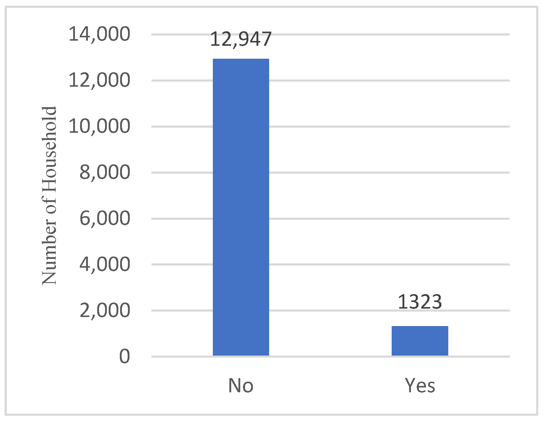
As shown in Figure 2, the label attribute was not balanced. Therefore, it was necessary to use the pre-processing method to avoid any misrepresentation of the minority class. In this paper, we split the dataset using 5-k fold cross-validation. Pre-processing sampling techniques, such as under- and over-sampling, were only used on the training set. SMOTE operator was the oversampling technique used. When creating synthetic samples for the dataset, SMOTE employs the k-NN approach by choosing the k nearest neighbors from sample data and connecting them. SMOTE may help the majority–minority class border become distinguishable since it solely relies on minority class observation. After the SMOTE process, the class label became balanced with Yes = 12,947 and No = 12,947. For RUS techniques, the operator Sample has been used with three different ratios; 1:1 (No = 1323, Yes = 1323), 2:1 (No = 2646, Yes = 1323), and 3:1 (No = 3969, Yes = 1323).
Step 4: Modelling—In this stage, five predictive models are used to predict whether the customer will purchase a life insurance policy. The classifiers include DT, LR, NB, RF, and ANN. Classifiers are chosen based on a literature review from past studies on data mining models and the five best models in ROC evaluation. In this paper, we propose to compare the full model without any sampling process with the models that have undergone resampling and ensembled process as follows; (i) five classifiers with different sampling techniques, (ii) classifiers with bagging ensemble learning method, and (iii) classifiers with boosting ensemble method.
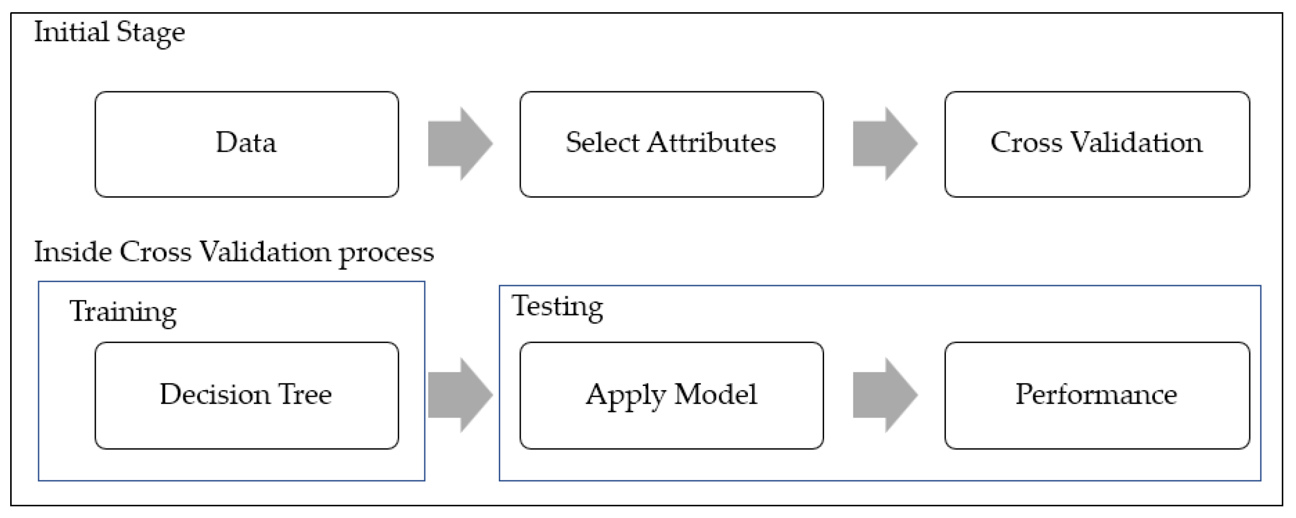
There are two stages in predictive modeling for life insurance ownership. Figure 3 illustrates the user interface of life insurance ownership modeling without the ensemble learning method used in this study. Many copies of the data were produced in the initial stage because the dataset needed to be connected with multiple classifiers. A 5-fold cross-validation strategy was also used to apply the model. The data file is called in the first interface, and the attributes are selected based on the explained attributes in Table 2 and Table 3. Next, the cross-validation operator with 5-fold validation is used. The “Cross Validation” operator, sometimes called a nested operator in RM, comprises the training and testing subprocesses. The dataset for this cross-validation process was divided into K (number of fold) subsets. Each iteration used one subset for testing, and the remaining dataset divisions were used for training. As the testing dataset was unseen, applying the model’s training and validation in one procedure was considered a fair test.
Next, the data are divided into training and testing inside the cross-validation operator. The input port (on the left) received the training dataset and connected with the DT, as shown in the figure. After the learning phase, the trained model was sent to the testing phase, where testing data were used to apply the testing procedure further. Finally, the model was verified using the “Apply Model” operator, which was connected to the “Performance” operator to help measure various characteristics of the classification model. Various parameters can be chosen for each of the classifiers in the RM. Hence, the authors experimented with various parameter combinations throughout implementation to evaluate the models’ performance. Then, the parameters with the highest accuracy are chosen. Similar to Figure 3, other classifiers with different sampling techniques adhere to the same process.
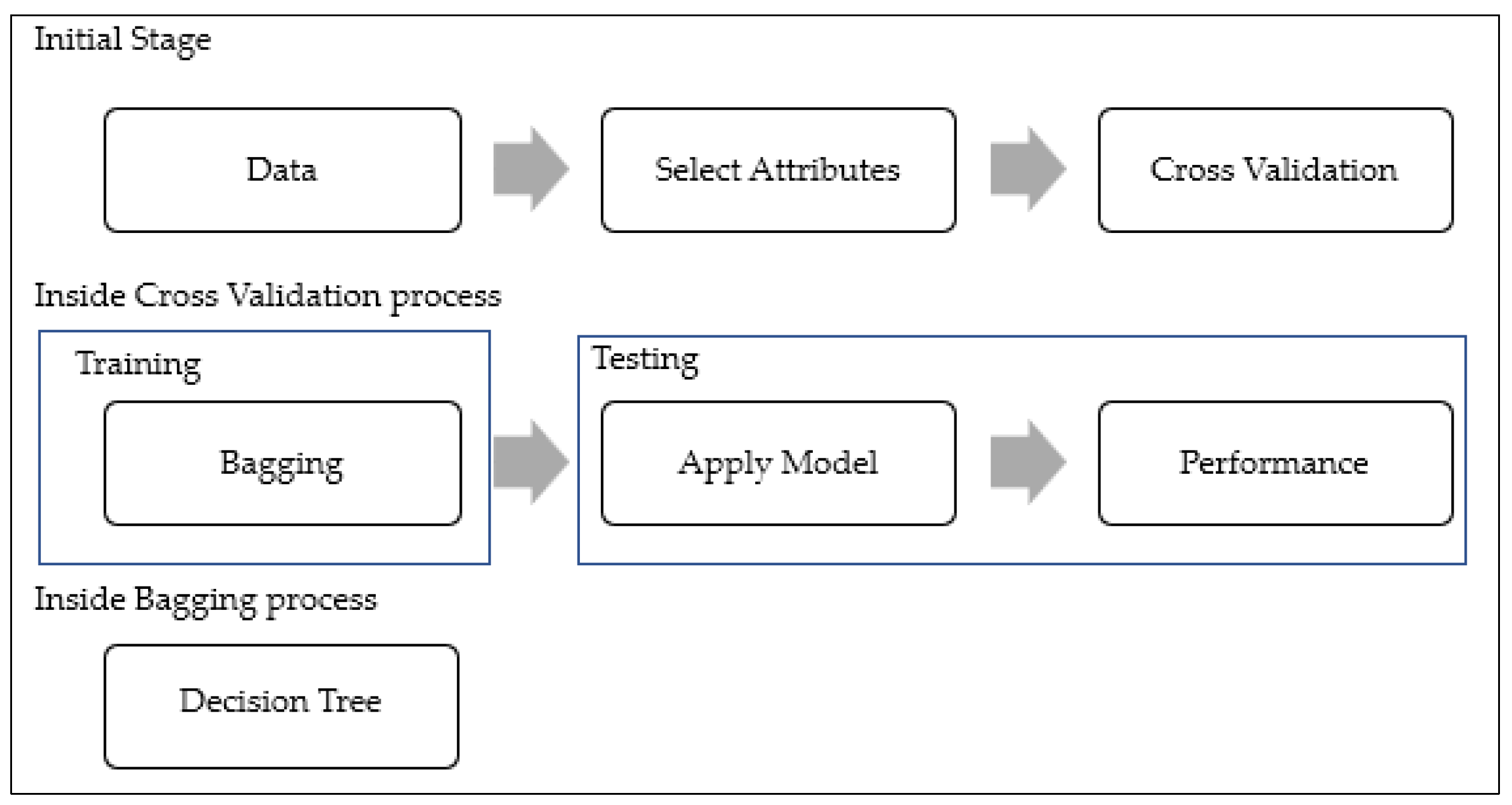
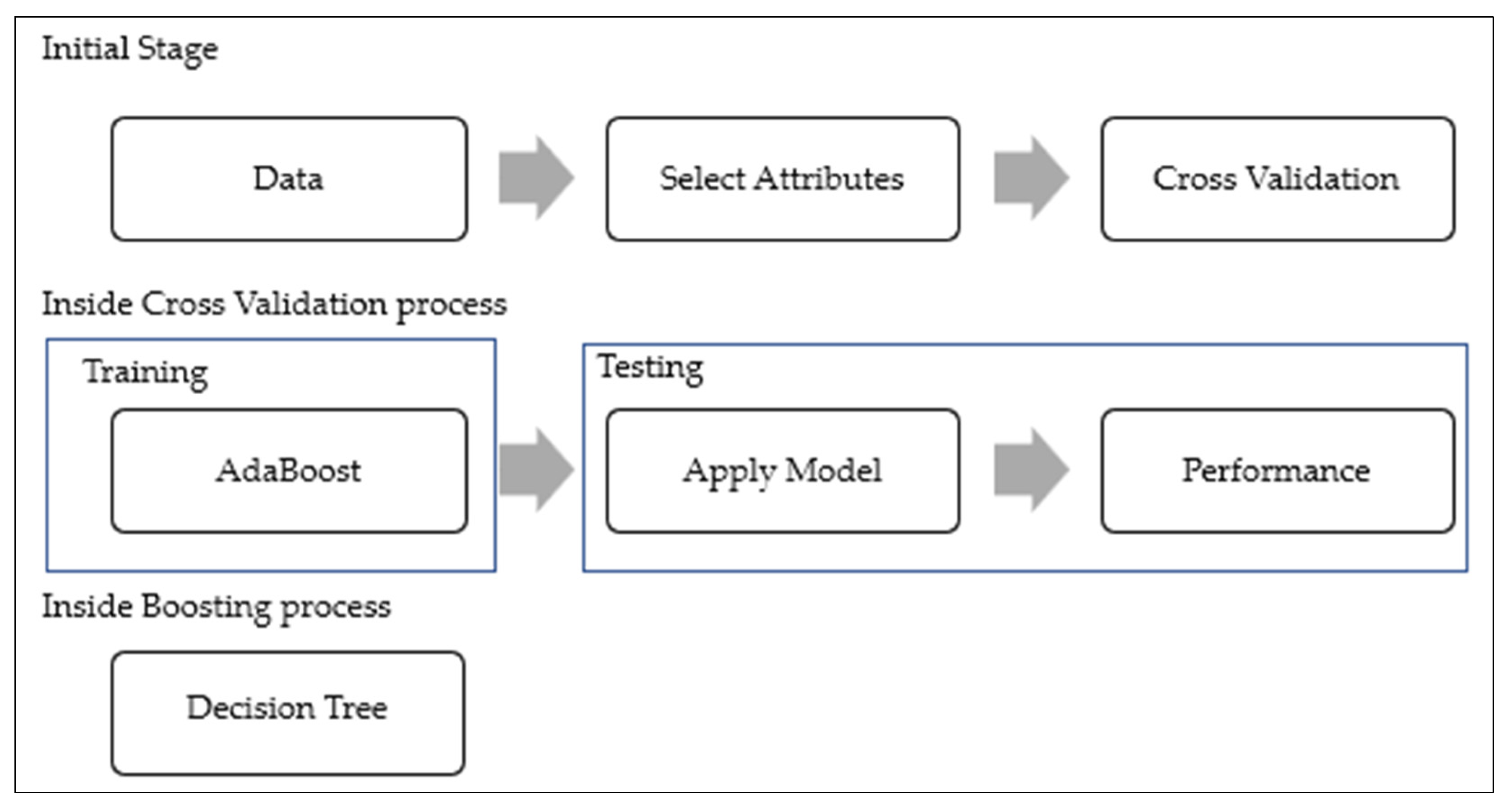
Meanwhile, the ensemble learning method is divided into three stages: (i) the initial stage, (ii) inside the cross-validation process, and (iii) inside the bagging/boosting process. Bagging and boosting (AdaBoost) were used as the ensemble learning method to see the differences in the performance metrics for each classifier. Figure 4 and Figure 5 demonstrate the implementation of bagging and boosting in the ensemble learning method. As for bagging, enhancing the performance of the classification model is the key motivation behind choosing this ensemble method [31]. A meta-algorithm known as bagging is renowned for its aggregation capabilities. The working scenario for this technique is based on bootstrapping, which separates the original dataset into numerous training datasets known as bootstraps. The datasets were divided to develop numerous models, which will eventually be combined to produce a powerful learner. The sub-process of this operator, which will use various learner models, is known as a nested operator.
Boosting is a popular ensemble strategy in machine learning that combines numerous models to obtain a robust model. It achieves this goal by merely training several learning models consecutively, then combining them based on discovered learning model errors. Besides that, according to research by Nazemi et al., boosting is helpful in reducing bias and variance [39]. One of the boosting algorithms that can be used with other learning algorithms is called AdaBoost, which stands for adaptive boosting [31]. The meta-algorithm used to implement AdaBoost in the RM tool can run the process by adding another algorithm as a sub-process. After running and training numerous models, it combines weak learners to form a single strong learner, adding extra calculation and running time. In this study, the classification model is trained using AdaBoost’s ensemble method that combines five additional algorithms as sub-processes. The primary goal of using AdaBoost is to compare decision-making models with and without boosted approaches in terms of performance and accuracy. The results and discussion section examines the model’s overall performance. Similar to Figure 4 and Figure 5, other classifiers with different sampling techniques follow the same process.
Step 5: Model Assessment and Comparison—In the final phase, it is necessary to evaluate the results and review the steps performed in detail [38]. The performance of each tested model was assessed using the confusion matrix, which includes the number of TP, FP, TN, and FN. The accuracy, precision, and recall measures can be calculated using these parameters. Accuracy measures the model’s ability to capture true positives as being positive and true negatives as being negatives. Precision is calculated by dividing the true positives by anything predicted as a positive. In contrast, Recall is calculated by dividing the true positives by anything that should have been predicted as positive. The formulas for the performance metrics used in our analysis are shown in Table 4.
The tools from which various accuracy measures are derived include an ROC chart and statistics such as accuracy, F1-score, and ROC index. Tékouabou, Alaoui, et al. (2022) [40] state that the F1-score balances recall and precision (also known as sensitivity), accounting for both minority and majority classes. Hence, it is one of the good indicators for choosing the best model for classification problems. Other useful metrics are BA and GM. BA is the average of the two rates for accurately classifying positive and negative events. Contrary to accuracy, the BA is strong for evaluating classifiers on imbalanced datasets [41]. GM is also an effective indicator for imbalanced data classification binary problems.

4. Discussion

This section will further discuss the result and analysis by describing the nature of the dataset, followed by the best model comparison.

4.1. Descriptive Analysis

As presented in Table 2, the average age for households involved in this dataset is 44.04. Most of the respondents are male (83.08%), as most of the heads of households in Malaysia are male. The income category was dominated by the B40 category, with 41.37%, followed by M40 (41.21%) and T20 (17.42%). More than half of the households are Bumiputera (67.34%), followed by Chinese (21.90%) and Indian (6.29%). Most families (47.18%) reside in a non-metropolitan area, and only 23.34% reside in a metropolitan area. Meanwhile, 29.49% live in East Malaysia. Besides that, only 4011 (28.11%) households have other than tertiary as the highest level of education, which concludes that the majority of the households taking part in this survey have tertiary as their highest level of education. Besides that, 57.11% of the households work in a white-collar industry. The prime age group (age 25 to 54), also known as the active working age group, appears to dominate, with 76.12%.
Table 5 shows the interval input summary. The average monthly household expenditure is RM 4187.44, with a minimum spending of RM 472.14. This shows that the average household in Malaysia falls in the B40 category. Meanwhile, most of the respondents have three members in a household.
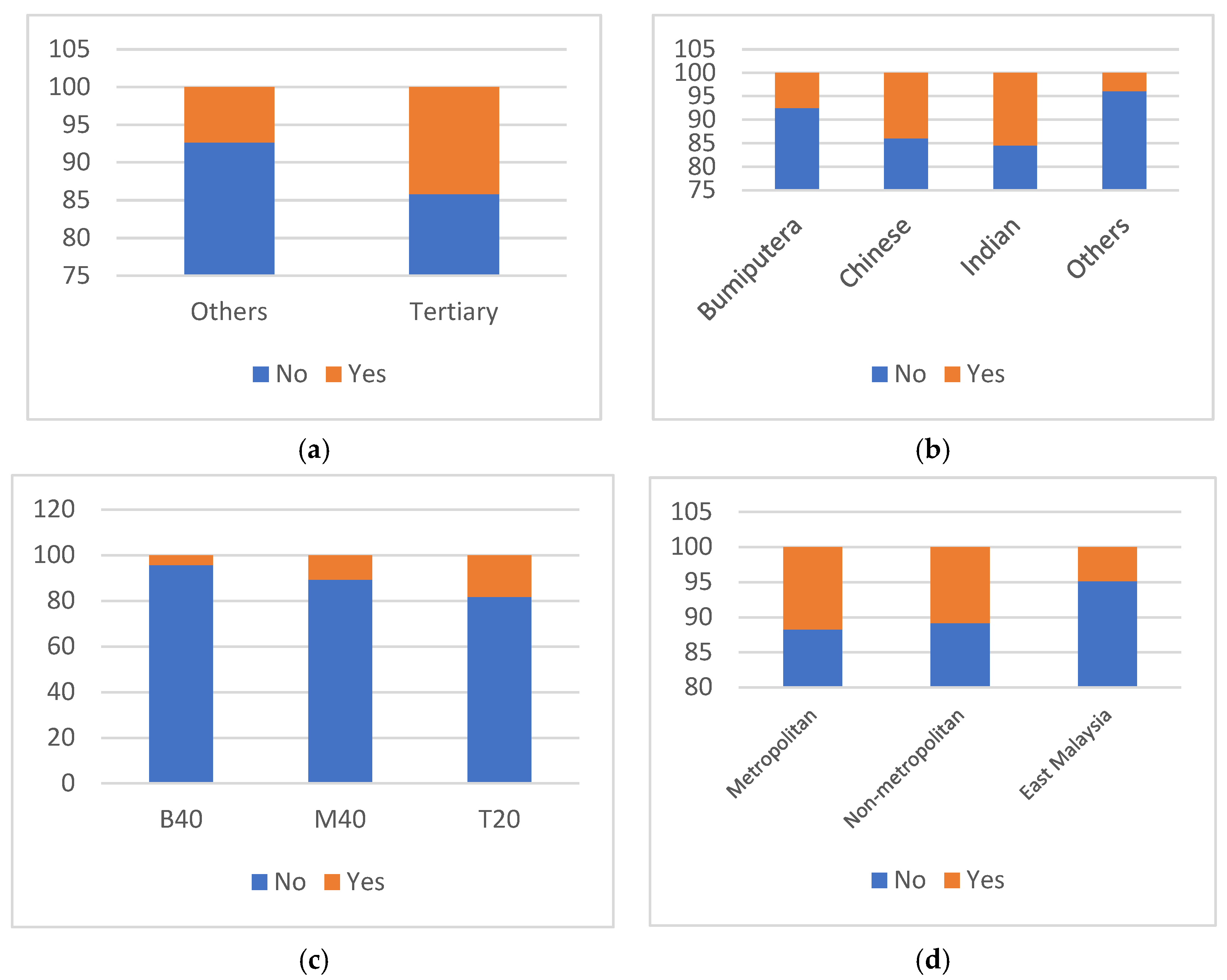
Figure 6 presents an overview of categorical attributes and perhaps indicators of the factors that should be paid particular attention to in determining life insurance ownership. The bar chart in Figure 6a demonstrates that those with tertiary education are more likely to own a life insurance policy than others. In contrast, Figure 6b shows that Chinese and Indian individuals outnumber Bumiputera individuals in life ownership status. Even though Bumiputera participants outnumber other ethnicities in this survey, as shown in Table 2, they do not contribute to the high percentage of life insurance ownership. It may be an indicator that Chinese and Indian individuals have more interest in owning a life insurance policy compared to Bumiputera. Figure 6c indicates that four times as many households in the highest 20% income levels will purchase life insurance policies as in the bottom 40%. The household in Figure 6d in a metropolitan area is likelier to have a life insurance policy than in a non-metropolitan location and East Malaysia.

4.2. Best Model Comparison

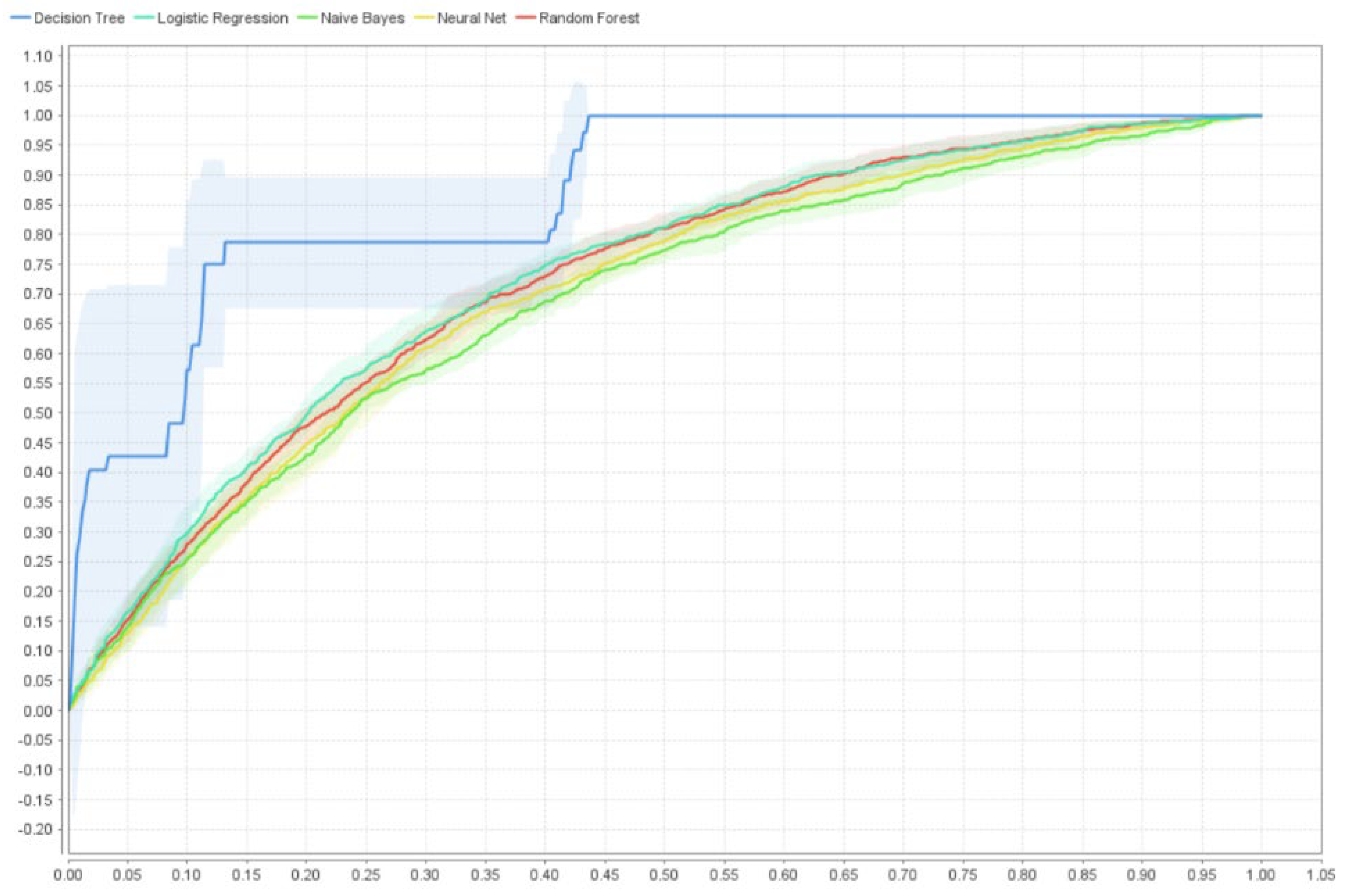
The area under the ROC curve is frequently used to evaluate the accuracy of classification models. A good model’s range value area under the curve (AUC) should be between 0.5 and 1. A greater AUC value will result in a more accurate model [18]. The classification classifiers used for the Compare ROCs were DT, NB, LR, RF, and ANN, using the whole dataset without modifying the data and sampling technique. This is to give an early overview of the performance of the model. The model accurately predicted the data if the curves’ climbed rapidly to the top-right [42]. Figure 7 presents each model’s ROC charts, showing that all models have almost the same performance except for the decision tree model. Based on Figure 7, it is recommended that if the researcher would like to use the whole dataset without considering the imbalanced data, then the decision tree would be the best classifier to use.
The summaries of the model comparison based on accuracy and balanced accuracy are presented in Table 6 and Table 7, respectively. It is shown that the bigger the difference between class labels, the more significantly the accuracy increased. This is due to there being too few data points for the model to learn from; the model tends to be biased towards the majority class and would be unable to identify fraud in the majority class. Classifiers with no sampling applied have the highest accuracy, the lowest at 86.06% and the highest at 90.66%, and classifiers with SMOTE have the lowest accuracy, ranging from 65.21% to 72.45%. Based on the accuracy, LR outperformed other classifiers with high accuracy rates for all the classifiers with different sampling and ensemble methods.
Meanwhile, NN has the highest accuracy rate in the SMOTE dataset, with and without the ensemble method. However, by looking at the balanced accuracy performance, NB showed the best model for an imbalanced dataset. Meanwhile, for the balanced dataset, RUS ratio 1:1 and SMOTE, LR showed the highest rate, with LR-SMOTE and LR + bagging SMOTE having slightly higher accuracy rates than other classifiers.
Table 8 represents the AUC index for all classifiers. LR showed consistent performances for all the models except classifiers with boosting ensemble. NB + boosting has the highest AUC (0.701) in RUS 1:1; other AUCs in boosting ensemble showed values less than 0.700. It can be observed that the AUC value for LR and LR + bagging and NB and NB + bagging has the same performance. The other models showed different values for the model without ensemble and the model with bagging ensemble.
In comparing the models with imbalanced datasets, F1 is also a good indicator, as presented in Table 9. F1 values showed that for a balanced dataset RUS ratio 1:1, LR + bagging is the best model, with a slightly higher performance, 0.2865, than LR + boosting and LR (0.2863 each, respectively). F1 values enable a model to be evaluated using a single score that accounts for precision and recall, which is useful when reporting model performance and comparing models.
Table 10 presents the GM values for all the models. Balanced datasets (SMOTE and RUS 1:1) performed better than the imbalanced dataset, with LR outperforming other models. Meanwhile, as shown in the table, the NB model outperformed the imbalanced dataset. GM is a metric that compares the classification performance of the majority and minority classes. A low GM indicates poor performance in categorizing positive cases, even if negative cases are successfully classified. LR and LR + boosting showed the same and highest GM performance of 0.6701, followed by LR + bagging, 0.6697.
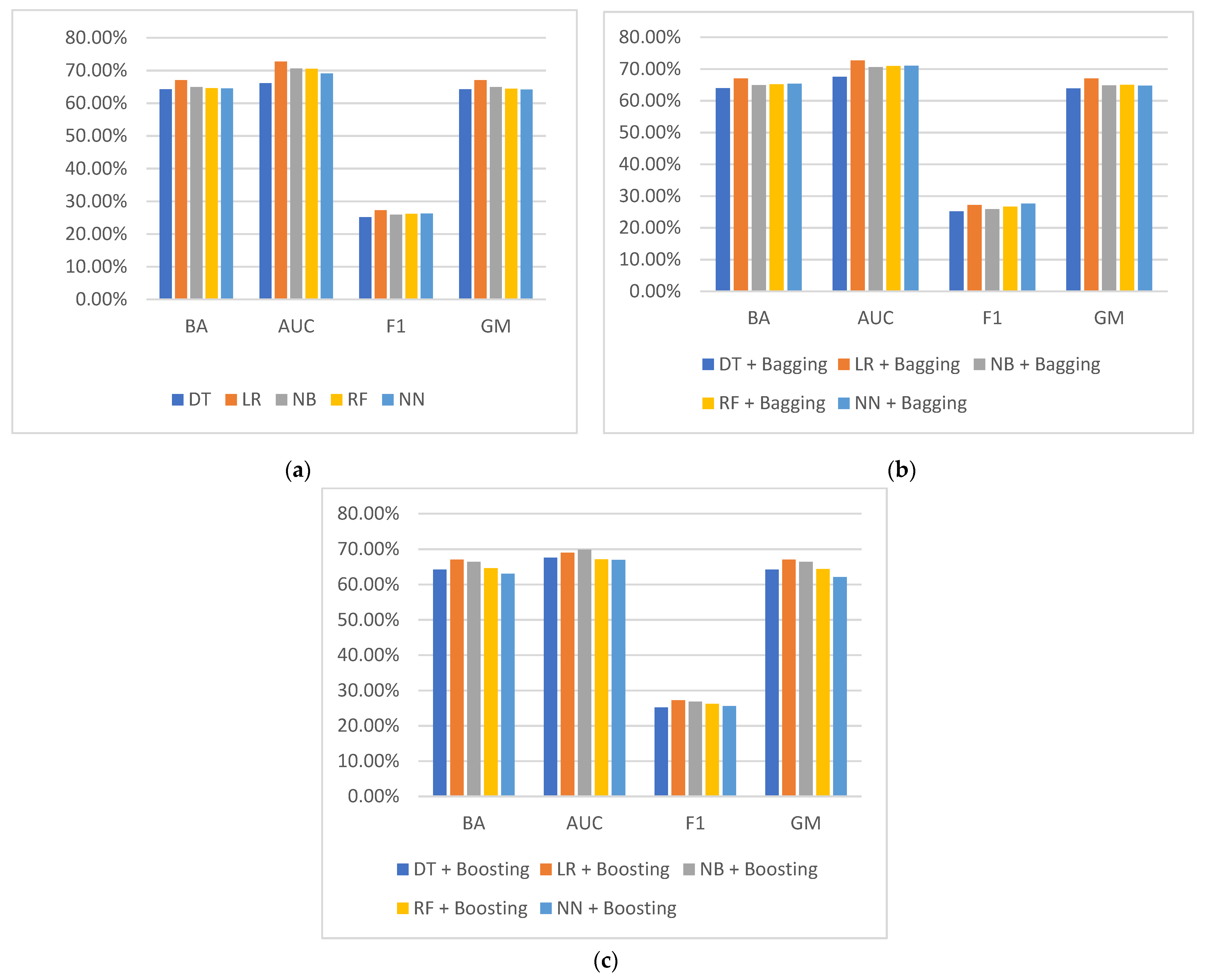
The overall model performance comparisons of SMOTE models without the ensemble learning method are presented in Figure 8a. Figure 8b illustrates the best model comparison in SMOTE for classifiers with the bagging ensemble learning method. In contrast, Figure 8c shows the best model comparison in SMOTE for classifiers with the boosting ensemble learning method. It can be seen in Figure 8a–c that the LR performances showed slightly higher performances in most performance criteria. However, in Figure 8c, Naïve Bayes showed better performances in AUC for classifiers with boosting ensemble. Regardless of whether the dataset used ensemble and sampling techniques or not in this dataset, the F1 scores showed almost the same performance, below 30%. The F1 scores might improve if the variables undergo feature selection [29], which can be interesting in future research. The study found that the SMOTE will perform better after feature selection.

4.3. Model Scoring

Considering all the performance metrics above, it is quite debatable which model is the best. The decision will depend on what one believes it means to have better performance. Based on Figure 8, LR showed slightly higher performances in all performance metrics, except for AUC, with boosting. Hence, we illustrate the Logistic Regression model for predicting life insurance purchasers in the model scoring step. Model scoring is performed to assess the accuracy and efficiency of the chosen model. Another dataset is used for the model scoring purpose. The dataset is another form of secondary data obtained from a DOSM, Malaysian Household Survey. Output for model scoring is as tabulated in Table 11.
Table 11 displays that a customer will be predicted to purchase a life insurance policy when the predicted value of Y = Yes is more than and equal to 0.5 and is predicted not to purchase when the person has a predicted value of Y = No more than or equal to 0.5. The prediction for observations 4, 5, and 10 would be incorrect. Meanwhile, other observations correctly predicted not to purchase life insurance. Thus, the model accuracy is 70%, and the prediction error rate is 0.3 (30%). The formula for the LR model to predict the life insurance purchaser is given as follows:
log p 1 p = 0.347 + 0.4488   I n c o m e   C a t e g o r y   T 20 + 0.5652   I n c o m e   C a t e g o r y   M 40 0.5818   M e t r o p o l i t a n 0.8716   E a s t   M a l a y s i a 0.2099   A g e   G r o u p 1 0.3700   R u r a l + 0.2199   M a l e + 0.2476   U n e m p l o y e d 0.3214   N o n W h i t e   C o l l a r 0.2123   h o u s e h o l d + 0.0002   ( e x p e n d i t u r e )  

5. Conclusions

Based on the results obtained in Section 4, it can be concluded that the performances of all classifiers that have undergone a sampling method are almost identical. SMOTE has slightly higher performance in balanced accuracy, AUC index, and GM. Even though the accuracy of the original dataset with no sampling applied has the highest accuracy value, other performance measurements showed the lowest. Hence, the imbalanced dataset proved to be highly accurate but misrepresented the majority class. Logistic Regression showed consistent performance with or without ensembled (bagging and boosting) for SMOTE and RUS 1:1. Even though the LR model in RUS 1:1 showed the highest value in F1 measures compared to other models, LR + SMOTE has been outperformed in most of the criteria. Hence, it can be concluded that SMOTE is the best sampling method [29], and it is pretty challenging to determine which model is the best to predict the potential life insurance purchasers in these data. Without feature selection in the dataset, LR has performed better, which is supported by Kaushik et al. [24] research. However, similar studies on classifying financial decisions show that nonlinear methods such as Neural Networks [24] and Random Forest [23] perform significantly better. Moreover, the analysis shows that the decision tree is the best performer according to ROC and, according to balanced accuracy, F1 score, and GM comparison, Naïve Bayes seems to be the best performer. Hence, the decision will depend on which performance criteria a researcher wishes to focus on.
By applying the ensembled method, we believe that it presented various performance comparisons. The performance of the ensembled models (bagging or boosting) significantly improves the models’ performances. However, the performances differ from one model to another. Based on the results discussed in Section 4.2, the researchers should evaluate each model with different ensembled methods to determine which classifier and ensemble method is appropriate for the dataset being studied. The findings of this study will be beneficial to society since insurance protection is important to the sustainability and financial well-being of families. It may help the insurance business select potential buyers more effectively through a better underwriting process. Additionally, this study will shed light on the prediction using various sampling and ensemble approaches throughout the classification process employing data mining techniques with an imbalanced dataset.
Despite the beneficial findings, this study has been conducted based on this limitation. It does not consider feature selection, which may affect the study’s outcome. Feature selection may provide a more thorough comparison, as it only considers the most significant attributes in the study. Perez et al. [29] stated that SMOTE performs better after applying feature selection. However, since this study aims to compare the different sampling and ensemble methods on the imbalanced dataset, the feature selection criteria have been excluded from this study. Hence, we recommend that future research considers the feature selection for a better understanding and comparison. This study proposes an approach to determine the usefulness of various artificial intelligence approaches using machine learning to predict life insurance ownership. This approach may also be used in countries with roughly identical life insurance penetration rates. Further improvements may also be achieved by including more socioeconomic status parameters and economic factors.

Author Contributions

Conceptualization, S.N.S. and N.I.; Methodology, S.N.S.; Software, S.N.S.; Supervision, N.I. and R.N.-F.; Visualization, S.N.S.; Writing—original draft, S.N.S.; Writing—review and editing, S.N.S., N.I. and R.N.-F. All authors have read and agreed to the published version of the manuscript.

Funding

This research was funded by Universiti Kebangsaan Malaysia, grant number GGPM-2020-016.

Institutional Review Board Statement

Not applicable.

Informed Consent Statement

Not applicable.

Data Availability Statement

Data are available upon reasonable request to the corresponding authors.

Acknowledgments

Siti Nurasyikin Shamsuddin would like to acknowledge the Ministry of Higher Education (MOHE) of Malaysia and Universiti Teknologi MARA (UiTM) for sponsoring her Ph.D. studies at Universiti Kebangsaan Malaysia (UKM) under Skim Latihan Akademik Bumiputera (SLAB).

Conflicts of Interest

The authors declare no conflict of interest. The funders had no role in the design of the study; in the collection, analyses, or interpretation of data; in the writing of the manuscript; or in the decision to publish the results.

References

  1. Hiwase, V.A.; Agrawal, A.J. Review on application of data mining in life insurance. Int. J. Eng. Technol. 2018, 7, 159–162. [Google Scholar] [CrossRef]
  2. Emamgholipour, S.; Arab, M.; Mohajerzadeh, Z. Life insurance demand: Middle East and North Africa. Int. J. Soc. Econ. 2017, 44, 521–529. [Google Scholar] [CrossRef]
  3. Swiss Re Institute. Closing Asia’s Mortality Protection Gap. Report; Swiss Re Institute: Zurich, Switzerland, 2020. [Google Scholar]
  4. Descombes, J. Why Hasn’t COVID-19 Led to an Increase in Life Insurance Protection? Available online: https://www.swissre.com/institute/research/topics-and-risk-dialogues/health-and-longevity/covid-19-life-insurance.html (accessed on 7 September 2022).
  5. LIMRA and Life Happens. 2021 Insurance Barometer Study, LIMRA and Life Happens. COVID-19 Drives Interest in Life Insurance; LIMRA: Windsor, CT, USA, 2021. [Google Scholar]
  6. Bank Negara Malaysia. Monthly Highlights and Statistics; Report; Bank Negara Malaysia: Kuala Lumpur, Malaysia, 2020. [Google Scholar]
  7. Swiss Re Institute. Sigma No. 4/2022: World Insurance:Inflation Risks Frontand Centre; Swiss Re Institute: Zurich, Switzerland, 2022. [Google Scholar]
  8. Bhatia, R.; Bhat, A.K.; Tikoria, J. Life insurance purchase behaviour: A systematic review and directions for future research. Int. J. Consum. Stud. 2021, 45, 1149–1175. [Google Scholar] [CrossRef]
  9. Annamalah, S. Profiling and purchasing decision of life insurance policies among married couples in Malaysia. World Appl. Sci. J. 2013, 23, 296–304. [Google Scholar]
  10. Grabova, P.; Sharku, G. Drivers of life insurance consumption—An empirical analysis of Western Balkan countries. Econ. Ann. 2021, 66, 33–58. [Google Scholar] [CrossRef]
  11. Loke, Y.J.; Goh, Y.Y. Purchase Decision of Life Insurance Policies among Malaysians. Int. J. Soc. Sci. Humanit. 2013, 2, 415–420. [Google Scholar] [CrossRef]
  12. Tan, A.K.G.; Yen, S.T.; Hasan, A.R.; Muhamed, K. Demand for Life Insurance in Malaysia: An Ethnic Comparison Using Household Expenditure Survey Data. Asia-Pac. J. Risk Insur. 2014, 8, 179–204. [Google Scholar] [CrossRef]
  13. Giri, M. A Behavioral Study of Life Insurance Purchase Decisions. Ph.D. Thesis, Indian Institute of Technology Kanpur, Kanpur, India, 2018. [Google Scholar]
  14. Kabrt, T. Life Insurance Demand Analysis: Evidence from Visegrad Group Countries. East. Eur. Econ. 2022, 60, 50–78. [Google Scholar] [CrossRef]
  15. Segodi, M.P.; Sibindi, A.B. Determinants of Life Insurance Demand: Empirical Evidence from BRICS Countries. Risks 2022, 10, 73. [Google Scholar] [CrossRef]
  16. Shamsuddin, S.N.; Ismail, N.; Roslan, N.F. What We Know about Research on Life Insurance Lapse: A Bibliometric Analysis. Risks 2022, 10, 97. [Google Scholar] [CrossRef]
  17. Gramegna, A.; Giudici, P. Why to buy insurance? An explainable artificial intelligence approach. Risks 2020, 8, 137. [Google Scholar] [CrossRef]
  18. Azzone, M.; Barucci, E.; Giuffra Moncayo, G.; Marazzina, D. A machine learning model for lapse prediction in life insurance contracts. Expert Syst. Appl. 2022, 191, 116261. [Google Scholar] [CrossRef]
  19. Yan, Y.; Xie, H. Research on the application of data mining technology in insurance informatization. In Proceedings of the 2009 9th International Conference on Hybrid Intelligent Systems, HIS 2009, Shenyang, China, 12–14 August 2009; Volume 3, pp. 202–205. [Google Scholar]
  20. Saidur Rahman, M.; Arefin, K.Z.; Masud, S.; Sultana, S.; Rahman, R.M. Analyzing Life Insurance Data with Different Classification Techniques for Customers’ Behavior Analysis. In Studies in Computational Intelligence; Springer Verlag: Berlin/Heidelberg, Germany, 2017; Volume 710, pp. 15–25. [Google Scholar]
  21. Abdul-Rahman, S.; Faiqah Kamal Arifin, N.; Hanafiah, M.; Mutalib, S. Customer Segmentation and Profiling for Life Insurance using K-Modes Clustering and Decision Tree Classifier. IJACSA Int. J. Adv. Comput. Sci. Appl. 2021, 12, 434–444. [Google Scholar] [CrossRef]
  22. Pereira, K.; Vinagre, J.; Alonso, A.N.; Coelho, F.; Carvalho, M. Privacy-Preserving Machine Learning in Life Insurance Risk Prediction. In Proceedings of the Joint European Conference on Machine Learning and Knowledge Discovery in Databases, Grenoble, France, 19–23 September 2022; Springer: Cham, Switzerland, 2023; Volume 1753, pp. 44–52. [Google Scholar]
  23. Rawat, S.; Rawat, A.; Kumar, D.; Sabitha, A.S. Application of machine learning and data visualization techniques for decision support in the insurance sector. Int. J. Inf. Manag. Data Insights 2021, 1, 100012. [Google Scholar] [CrossRef]
  24. Kaushik, K.; Bhardwaj, A.; Dwivedi, A.D.; Singh, R. Machine Learning-Based Regression Framework to Predict Health Insurance Premiums. Int. J. Environ. Res. Public Health 2022, 19, 7898. [Google Scholar] [CrossRef]
  25. Yap, C.T.; Khor, K.C. Utilising Sampling Methods to Improve the Prediction on Customers’ Buying Intention. In Proceedings of the 2022 International Conference on Decision Aid Sciences and Applications, DASA 2022, Chiangrai, Thailand, 23–25 March 2022; Institute of Electrical and Electronics Engineers Inc.: New York, NY, USA, 2022; pp. 352–356. [Google Scholar]
  26. Gonçalves, C.; Ferreira, D.; Neto, C.; Abelha, A.; Machado, J. Prediction of mental illness associated with unemployment using data mining. In Proceedings of the International Workshop on Healthcare Open Data, Intelligence and Interoperability (HODII), Madeira, Portugal, 2–5 November 2020; Elsevier B.V.: Amsterdam, The Netherlands, 2020; Volume 177, pp. 556–561. [Google Scholar]
  27. Tékouabou, S.C.K.; Gherghina, Ș.C.; Toulni, H.; Mata, P.N.; Martins, J.M. Towards Explainable Machine Learning for Bank Churn Prediction Using Data Balancing and Ensemble-Based Methods. Mathematics 2022, 10, 2379. [Google Scholar] [CrossRef]
  28. Díez-Pastor, J.F.; Rodríguez, J.J.; García-Osorio, C.; Kuncheva, L.I. Random Balance: Ensembles of variable priors classifiers for imbalanced data. Knowl. Based Syst. 2015, 85, 96–111. [Google Scholar] [CrossRef]
  29. Ramos-Pérez, I.; Arnaiz-González, Á.; Rodríguez, J.J.; García-Osorio, C. When is resampling beneficial for feature selection with imbalanced wide data? Expert Syst. Appl. 2022, 188, 116015. [Google Scholar] [CrossRef]
  30. Bauer, E.; Chan, P.; Stolfo, S.; Wolpert, D. An Empirical Comparison of Voting Classification Algorithms: Bagging, Boosting, and Variants. Mach. Learn. 1999, 36, 105–139. [Google Scholar] [CrossRef]
  31. Saleem, F.; Ullah, Z.; Fakieh, B.; Kateb, F. Intelligent decision support system for predicting student’s e-learning performance using ensemble machine learning. Mathematics 2021, 9, 2078. [Google Scholar] [CrossRef]
  32. Vafeiadis, T.; Diamantaras, K.I.; Sarigiannidis, G.; Chatzisavvas, K.C. A comparison of machine learning techniques for customer churn prediction. Simul. Model. Pract. Theory 2015, 55, 1–9. [Google Scholar] [CrossRef]
  33. Wang, Y.; Sherry, X.; Jennifer, N.; Priestley, L. Improving Risk Modeling Via Feature Selection, Hyper-Parameter Adjusting, and Model Ensembling. Glob. J. Econ. Financ. 2019, 3, 30–47. [Google Scholar]
  34. Kumar, D.R.; Sree, B.C.U.; Veera, K.; Manoj Kumar, V. Predicting heart disease using machine learning techniques. Int. Res. J. Comput. Sci. 2019, 6, 149–153. [Google Scholar]
  35. El-Khamisy Mohamed, N.; El-Bhrawy, A.S.M. Artificial Neural Networks in Data Mining. IOSR J. Comput. Eng. 2016, 18, 55–59. [Google Scholar]
  36. Prajwala, T.R. A Comparative Study on Decision Tree and Random Forest Using R Tool. Int. J. Adv. Res. Comput. Commun. Eng. 2015, 4, 196–199. [Google Scholar]
  37. Lakshmi, K.V.; Kumari, N.S. Survey on Naive Bayes Algorithm. Int. J. Adv. Res. Sci. Eng. 2018, 7, 240–246. [Google Scholar]
  38. Ferreira, D.; Silva, S.; Abelha, A.; Machado, J. Recommendation system using autoencoders. Appl. Sci. 2020, 10, 5510. [Google Scholar] [CrossRef]
  39. Nazemi, A.; Rezazadeh, H.; Fabozzi, F.J.; Höchstötter, M. Deep learning for modeling the collection rate for third-party buyers. Int. J. Forecast. 2022, 38, 240–252. [Google Scholar] [CrossRef]
  40. Tékouabou, S.C.K.; Alaoui, E.A.A.; Chabbar, I.; Toulni, H.; Cherif, W.; Silkan, H. Optimizing the early glaucoma detection from visual fields by combining preprocessing techniques and ensemble classifier with selection strategies. Expert Syst. Appl. 2022, 189, 115975. [Google Scholar] [CrossRef]
  41. De Diego, I.M.; Redondo, A.R.; Fernández, R.R.; Navarro, J.; Moguerza, J.M. General Performance Score for classification problems. Appl. Intell. 2022, 52, 12049–12063. [Google Scholar] [CrossRef]
  42. Ibrahim, S.; Khairi, S.S.M. Predictive Data Mining Approaches for Diabetes Mellitus Type II Disease. Int. J. Glob. Optim. Its Appl. 2022, 1, 126–134. [Google Scholar] [CrossRef]
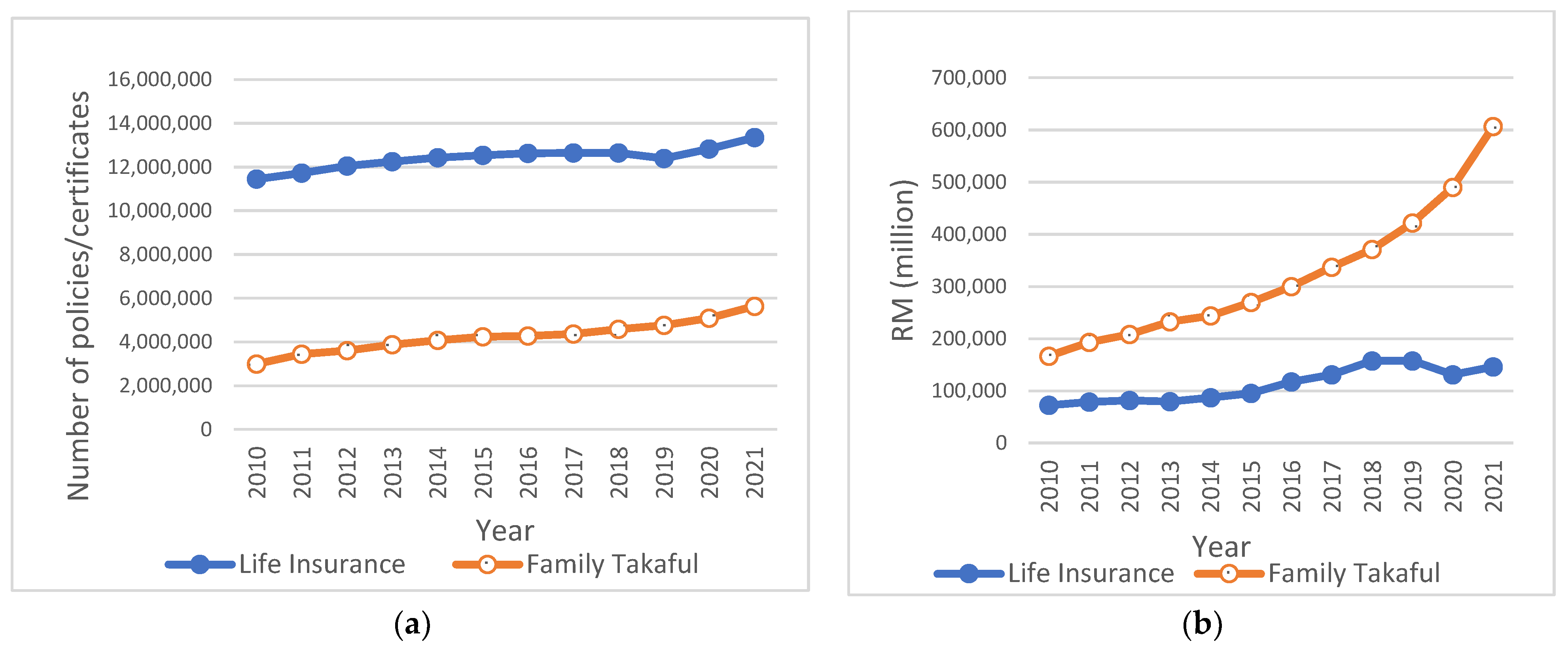
Figure 1. (a) Number of policies/certificates in force. (b) Distribution of new sums insured/sum participated.
Sustainability 15 10737 g001
Figure 2. Life insurance ownership distribution (target).
Sustainability 15 10737 g002
Figure 3. The RapidMiner’s user interface of life insurance ownership modeling without ensemble learning method.
Sustainability 15 10737 g003
Figure 4. The RapidMiner’s user interface of the life insurance modeling with bagging ensemble learning method.
Sustainability 15 10737 g004
Figure 5. The RapidMiner’s user interface of the life insurance ownership modeling with boosting ensemble learning method.
Sustainability 15 10737 g005
Figure 6. Percentages of life insurance ownership by (a) Education, (b) Ethnicity, (c) Income Category, and (d) Metropolitan Status.
Sustainability 15 10737 g006
Figure 7. ROC charts for model comparison without ensemble and sampling.
Sustainability 15 10737 g007
Figure 8. Best model comparison in SMOTE: (a) for classifiers without ensemble learning method, (b) for classifiers with bagging ensemble, and (c) for classifiers with boosting ensemble.
Sustainability 15 10737 g008
Table 1. The advantages and disadvantages of selected machine learning models.
ModelsAdvantagesDisadvantages
Decision Tree
  • The decision rules are simple to understand [34,36].
  • Nonparametric, therefore, there is no requirement to use unimodal training data, and it is simple to add a variety of numeric or categorical data layers [36].
  • Robust concerning training data outliers [36].
  • Decision trees frequently overfit training data, producing poor outcomes when used with the entire dataset [34,36].
  • Predictions beyond the response variable’s lowest and maximum limits in the training data are impossible [36].
  • Prone to overfitting [36].
Logistic Regression
  • It was created for classification purposes, and its greatest use is in determining how various independent factors affect a single outcome variable [34].
  • Works only if the predicted variable is binary [34].
  • Assumes all predictors are independent and data are free from missing values [34].
Naïve Bayes
  • Training and classification can be accomplished with one pass over the data [34].
  • Perform effectively in various real-world circumstances, including spam filtering and document classification [34,37].
  • Extremely rapid as compared to more advanced techniques [34].
  • Known to be a bad estimator [34].
  • Extremely strong assumption of independence that it makes. Finding such datasets in the actual world is quite difficult [37].
Random Forest
  • Provide accurate predictions for many applications [34,36].
  • Concerning the training dataset, it can measure the importance of each feature [36].
  • Biased for attributes with a different number of levels [36].
  • For binary variables, smaller groups are favored over larger groups if the data contain groups of correlated features [36].
  • A difficult technique and slow in real-time prediction [34].
Artificial Neural Network
  • Able to approximate complex non-linear mapping [35].
  • Flexible to incomplete and noisy data [35].
  • Do not make prior assumptions about the data distribution [35].
  • Overcome some limitations of other statistical methods while generalizing them [35].
  • The selection of the hidden nodes and training parameters is a heuristic [35].
  • Estimating the network weights can be very computationally intensive because it requires large data [35].
  • Useless to generalize new data if too many weights are used without regularization [35].
  • Confidence interval and hypothesis testing are unavailable, lacking classical statistical properties [35].
Table 2. Description of variables.
AttributesMeasurement LevelCategoryDescriptionFrequencyPercentage (%)
Life Insurance OwnershipBinaryYesHH has purchased a life insurance policy12,94790.73
NoHH has not purchased a life insurance policy13239.27
GenderBinaryMaleHH is male11,85683.08
FemaleHH is a female241416.92
AgeBinary1Non-prime working age340823.88
2Prime working age (25–54)10,86276.12
Income category (IC)NominalB40Household income is in the bottom 40% category *590441.37
M40Household income is in the middle 40% category *588041.21
T20Household income is in the top 20% category *248617.42
ExpenditureInterval-Household expenditure per month in Ringgit Malaysia --
Household Number (HN)Interval-Number of family members in the household--
Metropolitan Status (MS)NominalNon-MetropolitanResiding in the non-metropolitan West Malaysian673247.18
East MalaysiaResiding in the East Malaysian420829.49
MetropolitanResiding in the metropolitan West Malaysian333023.34
StrataBinaryUrbanResiding in an urban area10,88976.31
RuralResiding in a rural area338123.69
EthnicityNominalBumiputeraBumiputera960967.34
ChineseChinese312521.90
IndianIndian8986.29
OthersOthers6384.47
Marital Status (MS)NominalMarriedMarried10,73875.25
OthersOthers353224.75
Education Level (EL)NominalTertiaryHH’s highest level of education is a tertiary level10,25971.89
OthersHH’s highest level of education is other than tertiary401128.11
Employment Status (ES)BinaryEmployedHH is employed13,42694.09
UnemployedHH is unemployed8445.91
Collar Status (CS)BinaryWhite-collarHH has white-collar occupations (e.g., legislators, senior officials, managers, professionals);814957.11
Non-White collarHH has a non-white-collar occupation612142.89
Note 1. HH = Head of the household. Note 2. * DOSM classification of the income category.
Table 3. List of acronyms used.
AcronymsDefinitions
DTDecision Tree
LRLogistic Regression
NBNaïve Bayes
RFRandom Forest
NNNeural Network
k-NNk-Nearest Neighbours
SMOTESynthetic Minority Oversampling Technique
TPTrue Positive
TNTrue Negative
FPFalse Positive
FNFalse Negative
ROCReceiver Operating Characteristics
RUSRandom Under-Sampling
Table 4. Performance metrics used.
SymbolMetricFormula
ACCAccuracy(TP + TN)/(TP + TN + FP + FN)
BABalanced Accuracy(TPR + TNR)/2
GMGeometric Mean(TPR + TNR)1/2
F1F1-score2 × (Recall × Precision)/(Recall + Precision)
AUCArea Under the ROC CurvePlotted with TPR against the FPR
Note 1. TPR = sensitivity, TNR = specificity, FPR = false negative rate.
Table 5. Interval input summary.
AttributeMissingMeanStandard DeviationMinimumMaximumSkewnessKurtosis
Expenditure04187.4422450.359472.1417978.061.6424463.713083
Number of Households03.6683251.28989515−0.53572−0.91988
Table 6. Model’s accuracy comparison between different sampling and ensemble methods.
ModelNo Sampling
(Ratio 9:1)
RUS (Ratio 3:1)RUS (Ratio 2:1)RUS (Ratio 1:1)SMOTE
DT89.44%86.09%81.13%66.90%65.21%
LR90.66%89.21%86.26%73.40%66.32%
NB86.13%81.18%78.37%71.16%66.70%
RF90.50%88.35%82.93%68.19%69.19%
NN90.50%85.96%79.60%68.40%69.75%
DT + Bagging89.49%86.59%81.42%67.34%66.38%
LR + Bagging90.65%89.26%86.21%73.57%66.36%
NB + Bagging86.06%81.21%78.38%71.17%66.67%
RF + Bagging90.64%88.82%84.37%69.60%69.57%
NN + Bagging90.59%87.43%82.21%68.56%72.45%
DT + Boosting89.44%86.09%81.13%66.90%65.21%
LR + Boosting90.66%89.21%86.26%73.40%66.32%
NB + Boosting88.85%84.27%79.13%71.66%66.29%
RF + Boosting90.50%88.35%82.92%68.19%69.19%
NN + Boosting90.24%84.82%79.21%67.30%71.75%
Table 7. Model’s balanced accuracy comparison.
ModelNo Sampling
(Ratio 9:1)
RUS (Ratio 3:1)RUS (Ratio 2:1)RUS (Ratio 1:1)SMOTE
DT50.79%53.15%57.02%61.81%64.24%
LR50.13%53.61%57.99%66.27%67.02%
NB57.00%60.14%61.81%64.66%64.96%
RF50.42%53.47%56.32%64.25%64.63%
NN50.31%54.81%60.46%64.13%64.47%
DT + Bagging50.78%52.98%56.95%62.66%63.94%
LR + Bagging50.13%53.77%57.86%66.19%66.97%
NB + Bagging57.00%60.19%61.93%64.64%64.90%
RF + Bagging50.36%52.55%56.68%64.89%65.21%
NN + Bagging50.13%53.75%59.15%64.96%65.31%
DT + Boosting50.79%53.15%57.02%61.81%64.24%
LR + Boosting50.13%53.61%57.99%66.27%67.02%
NB + Boosting52.15%57.19%61.56%65.38%66.39%
RF + Boosting50.42%53.47%56.32%64.25%64.63%
NN + Boosting50.45%56.04%59.19%63.55%63.06%
Table 8. Model’s AUC index comparison.
ModelNo Sampling
(Ratio 9:1)
RUS (Ratio 3:1)RUS (Ratio 2:1)RUS (Ratio 1:1)SMOTE
DT0.6720.6600.6400.6210.661
LR0.7280.7270.7270.7270.727
NB0.7080.7080.7080.7070.706
RF0.6910.6920.6880.6940.705
NN0.7040.6980.6860.6830.691
DT + Bagging0.6780.6730.6720.6620.675
LR + Bagging0.7280.7270.7270.7270.727
NB + Bagging0.7080.7080.7080.7070.706
RF + Bagging0.6990.7040.7050.7100.709
NN + Bagging0.7230.7140.7130.7040.710
DT + Boosting0.5100.5480.6190.6670.676
LR + Boosting0.6930.6620.6600.6740.690
NB + Boosting0.6680.6840.6780.7010.699
RF + Boosting0.5060.5500.5990.6820.671
NN + Boosting0.6810.6720.6680.6740.670
Table 9. Model’s F1-score comparison.
ModelNo Sampling
(Ratio 9:1)
RUS (Ratio 3:1)RUS (Ratio 2:1)RUS (Ratio 1:1)SMOTE
DT0.05510.14470.21250.23700.2515
LR0.00740.14320.23820.28630.2722
NB0.22120.25250.26420.26720.2592
RF0.02300.14500.20390.25730.2618
NN0.01880.17850.25090.25670.2626
DT + Bagging0.05410.13960.21160.24410.2515
LR + Bagging0.00740.14730.23580.28650.2719
NB + Bagging0.22100.25320.26350.26710.2588
RF + Bagging0.01770.11770.21130.26500.2669
NN + Bagging0.00890.15410.24260.26320.2759
DT + Boosting0.05510.14470.21250.23700.2515
LR + Boosting0.00740.14320.23820.28630.2722
NB + Boosting0.10480.21570.26200.27470.2682
RF + Boosting0.02300.14500.20380.25720.2618
NN + Boosting0.02920.20050.23540.25070.2558
Table 10. Model’s GM comparison.
ModelNo Sampling
(Ratio 9:1)
RUS (Ratio 3:1)RUS (Ratio 2:1)RUS (Ratio 1:1)SMOTE
DT0.18090.34480.48740.61490.6423
LR0.06160.31040.46450.65690.6701
NB0.44390.54310.58370.64170.6492
RF0.10980.32020.45880.64070.6438
NN0.09880.39240.55700.63910.6414
DT + Bagging0.17870.33230.48370.62400.6386
LR + Bagging0.06160.31510.46210.65570.6697
NB + Bagging0.44440.54380.58540.64130.6486
RF + Bagging0.09530.27890.45340.64630.6499
NN + Bagging0.06700.34330.51930.64810.6471
DT + Boosting0.18090.34480.48740.61490.6423
LR + Boosting0.06160.31040.46450.65690.6701
NB + Boosting0.26270.46540.57650.64920.6639
RF + Boosting0.10980.32020.45870.64060.6438
NN + Boosting0.12570.43490.53840.63380.6214
Table 11. Summary of model scoring.
NoY StatusPredicted: Y = NoPredicted: Y = YesPrediction for Y
1Yes0.49880.5012Yes
2Yes0.30040.6996Yes
3Yes0.29710.7029Yes
4No0.26910.7309Yes
5No0.47740.5226Yes
6No0.58040.4196No
7No0.76650.2335No
8No0.63390.3661No
9No0.84180.1582No
10No0.42080.5792Yes
Disclaimer/Publisher’s Note: The statements, opinions and data contained in all publications are solely those of the individual author(s) and contributor(s) and not of MDPI and/or the editor(s). MDPI and/or the editor(s) disclaim responsibility for any injury to people or property resulting from any ideas, methods, instructions or products referred to in the content.