

Moderation of Clean Energy Innovation in the Relationship between the Carbon Footprint and Profits in CO₂e-Intensive Firms: A Quantitative Longitudinal Study


Abstract
1. Introduction
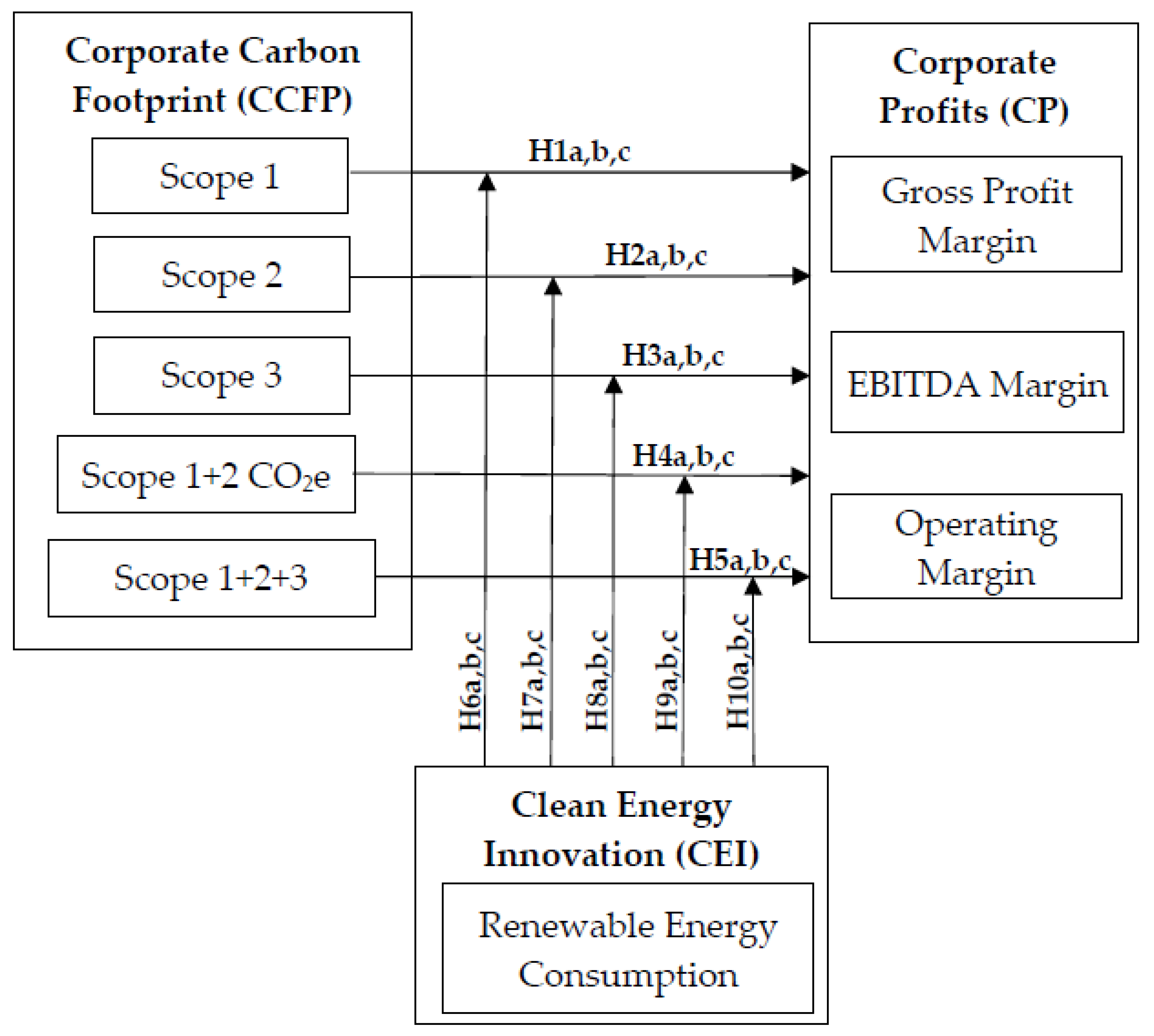
2. Theoretical Framework and Hypothesis
2.1. Corporate Carbon Footprint
2.2. Linking Corporate Carbon Footprint and Profits
2.3. Clean Energy Innovation
2.4. The Moderating Role of Clean Energy Innovation on the Relationship between Carbon Footprint and Profits
3. Research Methodology
3.1. Data and Sample
3.2. Data Collection
3.2.1. Corporate Carbon Footprint
3.2.2. Corporate Profits
3.2.3. Clean Energy Innovation
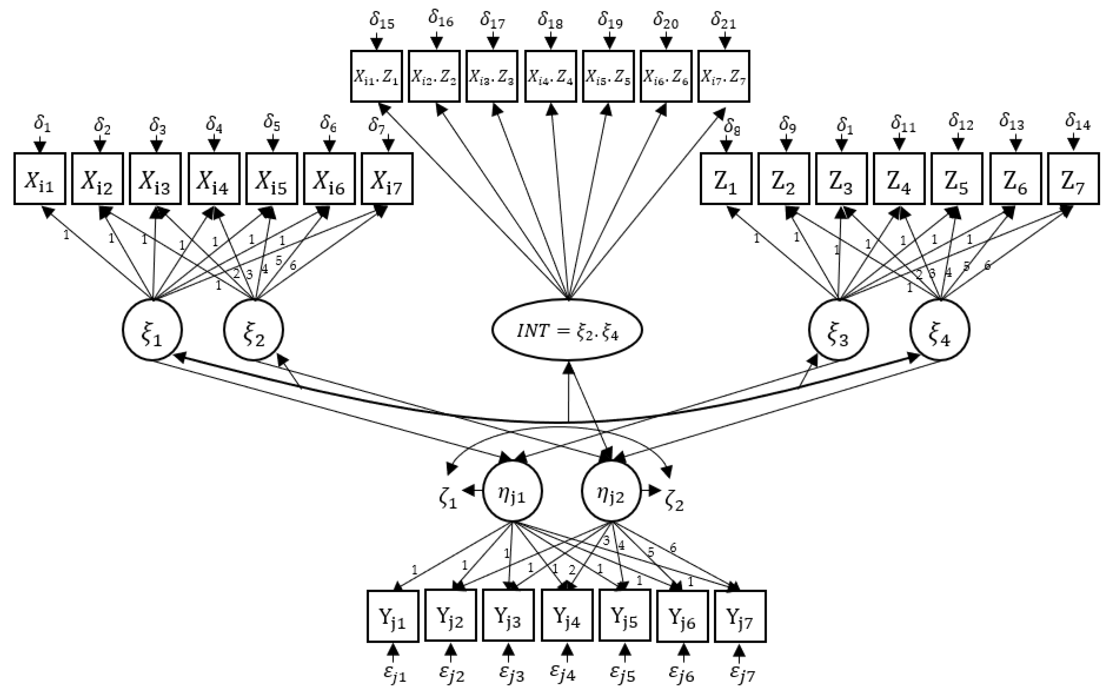
3.3. Data Analysis
Bayesian LGC Model Implemented
4. Empirical Results
4.1. Diagnostic Testing of B-LGC Model Fit
4.2. Hypothesis Testing
4.3. Graphic Illustrations of Longitudinal Moderating Effect
5. Discussion
6. Conclusions and Implications
Author Contributions
Funding
Data Availability Statement
Conflicts of Interest
Appendix A. Mplus-Specific Syntax for the B-LGC Model
| TITLE: Moderating Effect Analysis Based on the Bayesian Latent Growth Curve (LGC) Model | Title for the Bayesian analysis to be conducted. |
| DATA: FILE = w_Data2022_7.dat | Data file to be used: w_Data2022_7.dat is the name of this data file. |
| VARIABLE: | |
| NAMES ARE Firm_ID Sector X11 X12 X13 X14 X15 X16 X17 Z4 Z5 Z6 Z7 Y11 Y12 Y13 Y14 Y15 Y16 Y17; | Name of the seven time points (t = 7) of data for observable variables. We called them “X1t” here to represent seven metrics of Scope 1 emissions, “Zt” for renewable energy consumption (RENC) metrics, and “Y1t” for gross profit margin (Pr_Mrg). |
| USEVAR ARE X11 X12 X13 X14 X15 X16 X17 Z4 Z5 Z6 Z7 Y11 Y12 Y13 Y14 Y15 Y16 Y17; | |
| MISSING ARE ALL (−99). | |
| ANALYSIS: | |
| ESTIMATOR = BAYES; | Request the Bayesian estimator. |
| TYPE = RANDOM; | |
| POINT = MEAN; | Use of mean-centered indicators. |
| CHAINS = 3; | |
| PROCESSORS = 3; | |
| FBITERATIONS = 20000; | |
| BCONVERGENCE = 0.025; | |
| THIN = 30. | By specifying THIN = 30, we request that only every 30th iteration of the post-burn-in phase be used by Mplus to compute the posterior distribution. |
| MODEL: | Specification of the measurement model to be tested. |
| X11-X17*; | Estimation of residual variances for independent variable X1 (Scope 1) for each time point (t = 7). |
| Z1-Z7*; | Estimation of residual variances for moderator variable Z (RENC) for each time point (t = 7). |
| Y11-Y17*; | Estimation of residual variances for dependent variable Y1 (Pr_Mrg) for each time point (t = 7). |
| The asterisk (*) is used to a free estimation of residual variance parameters of independent variable (X1), moderating variable (Z), and dependent variable (Y1). | |
| KSI1 KSI2 | X11@0 X12@1 X13@2 X14@3 X15@4 X16@5 X17@6; | Specification of latent growth curve model with two latent growth parameters, intercepts (KSI1, KSI3 and ETA1), and slopes (KSI2, KSI4 and ETA2). All seven data time points (X11–X17, Z1–Z7, Y11–Y17) are used. The numbers to the right of @ indicate an equal time span between the data points, i.e., 0, 1, 2, 3, 4, 5, 6, and 7, reflecting equidistant points in time between 2015 and 2021) |
| KSI3 KSI4 | Z1@0 Z2@1 Z3@2 Z4@3 Z5@4 Z6@5 Z7@6; | |
| ETA1 ETA2 | Y11@0 Y12@1 Y13@2 Y14@3 Y15@4 Y16@5 Y17@6; | |
| KSI1*; KSI2*; KSI3*; KSI4*; ETA1*; ETA2*; | Estimation of variances of latent growth parameters. |
| INT1 | KSI1 XWITH KSI3; | Definition of interaction (moderation) term. INT1 corresponds to the latent product variable between intersections KSI1 and KSI3. |
| INT2 | KSI2 XWITH KSI4; | Definition of interaction (moderation). INT2 corresponds to the latent product variable between slopes KSI2 and KSI4. |
| ETA1 ON KSI1 KSI3 INT1; | Structural model specification. |
| ETA2 ON KSI2 KSI4 INT2. | Structural model specification. |
| OUTPUT: CINTERVAL(hpd) TECH8 STDYX. | |
| PLOT: TYPE = PLOT2. | |
| by S. Depaoli, H. M. Rus, J. P. Clifton, R. van de Schoot, & J. Tiemensma, 2017, Health Psychology Review, 11(3), 248–264. [76]. | |
References
- Cadez, S.; Czerny, A.; Letmathe, P. Stakeholder pressures and corporate climate change mitigation strategies. Bus. Strategy Environ. 2019, 28, 1–14. [Google Scholar] [CrossRef]
- Rissman, J.; Bataille, C.; Masanet, E.; Aden, N.; Morrow, W.R.; Zhou, N.; Elliott, N.; Dell, R.; Heeren, N.; Huckestein, B.; et al. Technologies and policies to decarbonize global industry: Review and assessment of mitigation drivers through 2070. Appl. Energy 2020, 266, 114848. [Google Scholar] [CrossRef]
- Wimbadi, R.W.; Djalante, R. From decarbonization to low carbon development and transition: A systematic literature review of the conceptualization of moving toward net-zero carbon dioxide emission (1995–2019). J. Clean. Prod. 2020, 256, 120307. [Google Scholar] [CrossRef]
- Damert, M.; Baumgartner, R.J. Intra-Sectoral Differences in Climate Change Strategies: Evidence from the Global Automotive Industry. Bus. Strategy Environ. 2018, 27, 265–281. [Google Scholar] [CrossRef] [PubMed]
- Boiral, O.; Henri, J.-F.; Talbot, D. Modeling the Impacts of Corporate Commitment on Climate Change. Bus. Strategy Environ. 2011, 21, 495–516. [Google Scholar] [CrossRef]
- Lewandowski, S.; Ullrich, A. Measures to reduce corporate GHG emissions: A review-based taxonomy and survey-based cluster analysis of their application and perceived effectiveness. J. Environ. Manag. 2023, 325, 116437. [Google Scholar] [CrossRef]
- Wang, L.; Li, S.; Gao, S. Do Greenhouse Gas Emissions Affect Financial Performance?—An Empirical Examination of Australian Public Firms. Bus. Strategy Environ. 2013, 23, 505–519. [Google Scholar] [CrossRef]
- Wesseling, J.; Lechtenböhmer, S.; Åhman, M.; Nilsson, L.; Worrell, E.; Coenen, L. The transition of energy intensive processing industries towards deep decarbonization: Characteristics and implications for future research. Renew. Sustain. Energy Rev. 2017, 79, 1303–1313. [Google Scholar] [CrossRef]
- Wright, C.; Nyberg, D. An Inconvenient Truth: How Organizations Translate Climate Change into Business as Usual. Acad. Manag. J. 2017, 60, 1633–1661. [Google Scholar] [CrossRef]
- BP. Advancing the Energy Transition; BP p.l.c: London, UK, 2018; pp. 1–28. [Google Scholar]
- Chevron. Climate Change Resilience: A Framework for Decision Making; Chevron Corporation: San Ramon, CA, USA, 2018; pp. 1–47. [Google Scholar]
- Shell. Shell Energy Transition Report; Shell p.l.c: London, UK, 2018; pp. 1–41. [Google Scholar]
- Capurso, T.; Stefanizzi, M.; Torresi, M.; Camporeale, S. Perspective of the role of hydrogen in the 21st century energy transition. Energy Convers. Manag. 2021, 251, 114898. [Google Scholar] [CrossRef]
- Yan, X.; He, Y.; Fan, A. Carbon footprint prediction considering the evolution of alternative fuels and cargo: A case study of Yangtze river ships. Renew. Sustain. Energy Rev. 2023, 173, 113068. [Google Scholar] [CrossRef]
- Castro, P.; Gutiérrez-López, C.; Tascón, M.T.; Castaño, F.J. The impact of environmental performance on stock prices in the green and innovative context. J. Clean. Prod. 2021, 320, 128868. [Google Scholar] [CrossRef]
- Galama, J.T.; Scholtens, B. A meta-analysis of the relationship between companies’ greenhouse gas emissions and financial performance. Environ. Res. Lett. 2021, 16, 043006. [Google Scholar] [CrossRef]
- Robaina, M.; Madaleno, M. The relationship between emissions reduction and financial performance: Are Portuguese companies in a sustainable development path? Corp. Soc. Responsib. Environ. Manag. 2020, 27, 1213–1226. [Google Scholar] [CrossRef]
- Russo, A.; Pogutz, S.; Misani, N. Paving the road toward eco-effectiveness: Exploring the link between greenhouse gas emissions and firm performance. Bus. Strategy Environ. 2021, 30, 3065–3078. [Google Scholar] [CrossRef]
- Wedari, L.K.; Moradi-Motlagh, A.; Jubb, C. The moderating effect of innovation on the relationship between environmental and financial performance: Evidence from high emitters in Australia. Bus. Strategy Environ. 2023, 32, 654–672. [Google Scholar] [CrossRef]
- Zhou, Y.; Shu, C.; Jiang, W.; Gao, S. Green management, firm innovations, and environmental turbulence. Bus. Strategy Environ. 2019, 28, 567–581. [Google Scholar] [CrossRef]
- Hang, M.; Geyer-Klingeberg, J.; Rathgeber, A.W. It is merely a matter of time: A meta-analysis of the causality between environmental performance and financial performance. Bus. Strategy Environ. 2019, 28, 257–273. [Google Scholar] [CrossRef]
- Bai, C.; Feng, C.; Du, K.; Wang, Y.; Gong, Y. Understanding spatial-temporal evolution of renewable energy technology innovation in China: Evidence from convergence analysis. Energy Policy 2020, 143, 111570. [Google Scholar] [CrossRef]
- Zhang, F.; Tang, T.; Su, J.; Huang, K. Inter-sector network and clean energy innovation: Evidence from the wind power sector. J. Clean. Prod. 2020, 263, 121287. [Google Scholar] [CrossRef]
- Mol, A.P.J. Ecological Modernization and the Global Economy. Glob. Environ. Politics 2002, 2, 92–115. [Google Scholar] [CrossRef]
- Mol, A.P. Ecological Modernisation around the World: Perspectives and Critical Debates. Environ. Manag. Health 2000, 11, 475–476. [Google Scholar] [CrossRef]
- Hart, S.L. A Natural-Resource-Based View of the Firm. Acad. Manag. Rev. 1995, 20, 986–1014. [Google Scholar] [CrossRef]
- Nguyen, Q.; Diaz-Rainey, I.; Kuruppuarachchi, D. Predicting corporate carbon footprints for climate finance risk analyses: A machine learning approach. Energy Econ. 2021, 95, 105129. [Google Scholar] [CrossRef]
- Busch, T.; Lewandowski, S. Corporate Carbon and Financial Performance: A Meta-analysis. J. Ind. Ecol. 2018, 22, 745–759. [Google Scholar] [CrossRef]
- Dahlmann, F.; Branicki, L.; Brammer, S. Managing Carbon Aspirations: The Influence of Corporate Climate Change Targets on Environmental Performance. J. Bus. Ethics 2019, 158, 1–24. [Google Scholar] [CrossRef]
- Harangozo, G.; Szigeti, C. Corporate carbon footprint analysis in practice—With a special focus on validity and reliability issues. J. Clean. Prod. 2017, 167, 1177–1183. [Google Scholar] [CrossRef]
- Lewandowski, S. Corporate Carbon and Financial Performance: The Role of Emission Reductions. Bus. Strategy Environ. 2017, 26, 1196–1211. [Google Scholar] [CrossRef]
- WBCSD; WRI. The GHG Protocol Corporate Accounting and Reporting Standard, Revised ed.; World Business Council for Sustainable Development (WBSCD): Geneva, Switzerland; World Resources Institute (WRI): Washington, DC, USA, 2015; pp. 1–116. [Google Scholar]
- Yagi, M.; Managi, S. Decomposition analysis of corporate carbon dioxide and greenhouse gas emissions in Japan: Integrating corporate environmental and financial performances. Bus. Strategy Environ. 2018, 27, 1476–1492. [Google Scholar] [CrossRef]
- WBCSD; WRI. Technical Guidance for Calculating Scope 3 Emissions (Version1.0): Supplement to the Corporate Value Chain (Scope 3) Accounting & Reporting Standard; World Business Council for Sustainable Development (WBSCD): Geneva, Switzerland; World Resources Institute (WRI): Washington, DC, USA, 2013; pp. 1–182. [Google Scholar]
- WBCSD; WRI. The GHG Protocol the Corporate Value Chain (Scope 3) Accounting and Reporting Standard; World Business Council for Sustainable Development (WBSCD): Geneva, Switzerland; World Resources Institute (WRI): Washington, DC, USA, 2011; pp. 1–152. [Google Scholar]
- Barney, J. Firm Resources and Sustained Competitive Advantage. J. Manag. 1991, 17, 99–120. [Google Scholar] [CrossRef]
- Freeman, R.E. Strategic Management: A Stakeholder Approach; Pitman: London, UK, 1984; Volume 4. [Google Scholar]
- Penz, E.; Polsa, P. How do companies reduce their carbon footprint and how do they communicate these measures to stakeholders? J. Clean. Prod. 2018, 195, 1125–1138. [Google Scholar] [CrossRef]
- Tuesta, Y.N.; Soler, C.C.; Feliu, V.R. Carbon management accounting and financial performance: Evidence from the European Union emission trading system. Bus. Strategy Environ. 2021, 30, 1270–1282. [Google Scholar] [CrossRef]
- Shahgholian, A. Unpacking the relationship between environmental profile and financial profile; literature review toward methodological best practice. J. Clean. Prod. 2019, 233, 181–196. [Google Scholar] [CrossRef]
- Kim, S.; Terlaak, A.; Potoski, M. Corporate sustainability and financial performance: Collective reputation as moderator of the relationship between environmental performance and firm market value. Bus. Strategy Environ. 2021, 30, 1689–1701. [Google Scholar] [CrossRef]
- Busch, T.; Bassen, A.; Lewandowski, S.; Sump, F. Corporate Carbon and Financial Performance Revisited. Organ. Environ. 2022, 35, 154–171. [Google Scholar] [CrossRef]
- Broadstock, D.C.; Collins, A.; Hunt, L.C.; Vergos, K. Voluntary disclosure, greenhouse gas emissions and business performance: Assessing the first decade of reporting. Br. Account. Rev. 2017, 50, 48–59. [Google Scholar] [CrossRef]
- Gallagher, K.S.; Holdren, J.P.; Sagar, A.D. Energy-Technology Innovation. Annu. Rev. Environ. Resour. 2006, 31, 193–237. [Google Scholar] [CrossRef]
- Horbach, J.; Rammer, C. Energy transition in Germany and regional spill-overs: The diffusion of renewable energy in firms. Energy Policy 2018, 121, 404–414. [Google Scholar] [CrossRef]
- Nelson, R.; Sidney, W. An Evolutionary Theory of Economic Change; Belknap Press, Ed.; Harvard University Press: Cambridge, MA, USA, 1982. [Google Scholar]
- Spaargaren, G. The Ecological Modernization of Production and Consumption; Essays in Environmental Sociology/G. Spaargaren - [S.I.: s.n.]. Ph. D. Thesis, Landbouw Universiteit, Wageningen, The Netherlands, 1997. [Google Scholar]
- Ruttan, V.W. Induced Innovation, Evolutionary Theory and Path Dependence: Sources of Technical Change. Econ. J. 1997, 107, 1520–1529. [Google Scholar] [CrossRef]
- Porter, M.E.; Linde, C.V.D. Green and Competitive: Ending the Stalemate Green and Competitive. Harv. Bus. Rev. 1995, 33, 120–134. [Google Scholar]
- Busch, J.; Foxon, T.J.; Taylor, P.G. Designing industrial strategy for a low carbon transformation. Environ. Innov. Soc. Transit. 2018, 29, 114–125. [Google Scholar] [CrossRef]
- Jänicke, M. Ecological modernisation: New perspectives. J. Clean. Prod. 2008, 16, 557–565. [Google Scholar] [CrossRef]
- Demirel, P.; Kesidou, E. Sustainability-oriented capabilities for eco-innovation: Meeting the regulatory, technology, and market demands. Bus. Strategy Environ. 2019, 28, 847–857. [Google Scholar] [CrossRef]
- Alvarez, S.; Carballo-Penela, A.; Mateo-Mantecón, I.; Rubio, A. Strengths-Weaknesses-Opportunities-Threats analysis of carbon footprint indicator and derived recommendations. J. Clean. Prod. 2016, 121, 238–247. [Google Scholar] [CrossRef]
- Ding, L.; Ye, R.M.; Wu, J.-X. Platform strategies for innovation ecosystem: Double-case study of Chinese automobile manufactures. J. Clean. Prod. 2019, 209, 1564–1577. [Google Scholar] [CrossRef]
- Lin, W.-L.; Cheah, J.-H.; Azali, M.; Ho, J.A.; Yip, N. Does firm size matter? Evidence on the impact of the green innovation strategy on corporate financial performance in the automotive sector. J. Clean. Prod. 2019, 229, 974–988. [Google Scholar] [CrossRef]
- Haney, A.B. Threat Interpretation and Innovation in the Context of Climate Change: An Ethical Perspective. J. Bus. Ethics 2017, 143, 261–276. [Google Scholar] [CrossRef]
- Fernández-Cuesta, C.; Castro, P.; Tascón, M.T.; Castaño, F.J. The effect of environmental performance on financial debt. European evidence. J. Clean. Prod. 2019, 207, 379–390. [Google Scholar] [CrossRef]
- Shahab, Y.; Ntim, C.G.; Chengang, Y.; Ullah, F.; Fosu, S. Environmental policy, environmental performance, and financial distress in China: Do top management team characteristics matter? Bus. Strategy Environ. 2018, 27, 1635–1652. [Google Scholar] [CrossRef]
- Hertwich, E.G.; Peters, G.P. Carbon Footprint of Nations: A Global, Trade-Linked Analysis. Environ. Sci. Technol. 2009, 43, 6414–6420. [Google Scholar] [CrossRef]
- Bataille, C.; Åhman, M.; Neuhoff, K.; Nilsson, L.J.; Fischedick, M.; Lechtenböhmer, S.; Solano-Rodriquez, B.; Denis-Ryan, A.; Stiebert, S.; Waisman, H.; et al. A review of technology and policy deep decarbonization pathway options for making energy-intensive industry production consistent with the Paris Agreement. J. Clean. Prod. 2018, 187, 960–973. [Google Scholar] [CrossRef]
- Smith, W.L.; Hillon, Y.C.; Liang, Y. Reassessing measures of sustainable firm performance: A consultant’s guide to identifying hidden costs in corporate disclosures. Bus. Strategy Environ. 2019, 28, 353–365. [Google Scholar] [CrossRef]
- Rentschler, J.; Kornejew, M. Energy price variation and competitiveness: Firm level evidence from Indonesia. Energy Econ. 2017, 67, 242–254. [Google Scholar] [CrossRef]
- Makridou, G.; Doumpos, M.; Galariotis, E. The financial performance of firms participating in the EU emissions trading scheme. Energy Policy 2019, 129, 250–259. [Google Scholar] [CrossRef]
- Jackson, J.; Belkhir, L. Assigning firm-level GHGE reductions based on national goals—Mathematical model & empirical evidence. J. Clean. Prod. 2018, 170, 76–84. [Google Scholar] [CrossRef]
- Maama, H.; Doorasamy, M.; Rajaram, R. Cleaner production, environmental and economic sustainability of production firms in South Africa. J. Clean. Prod. 2021, 298, 126707. [Google Scholar] [CrossRef]
- Velte, P.; Stawinoga, M.; Lueg, R. Carbon performance and disclosure: A systematic review of governance-related determinants and financial consequences. J. Clean. Prod. 2020, 254, 120063. [Google Scholar] [CrossRef]
- Pons, M.; Bikfalvi, A.; Llach, J.; Palcic, I. Exploring the impact of energy efficiency technologies on manufacturing firm performance. J. Clean. Prod. 2013, 52, 134–144. [Google Scholar] [CrossRef]
- Gallagher, K.S.; Anadon, L.D.; Kempener, R.; Wilson, C. Trends in investments in global energy research, development, and demonstration. WIREs Clim. Chang. 2011, 2, 373–396. [Google Scholar] [CrossRef]
- Cheng, Y.; Yao, X. Carbon intensity reduction assessment of renewable energy technology innovation in China: A panel data model with cross-section dependence and slope heterogeneity. Renew. Sustain. Energy Rev. 2021, 135, 110157. [Google Scholar] [CrossRef]
- Zhang, F.; Gallagher, K.S.; Myslikova, Z.; Narassimhan, E.; Bhandary, R.R.; Huang, P. From fossil to low carbon: The evolution of global public energy innovation. WIREs Clim. Chang. 2021, 12, e734. [Google Scholar] [CrossRef]
- Trencher, G.; Rinscheid, A.; Rosenbloom, D.; Truong, N. The rise of phase-out as a critical decarbonisation approach: A systematic review. Environ. Res. Lett. 2022, 17, 123002. [Google Scholar] [CrossRef]
- Yang, F.; Cheng, Y.; Yao, X. Influencing factors of energy technical innovation in China: Evidence from fossil energy and renewable energy. J. Clean. Prod. 2019, 232, 57–66. [Google Scholar] [CrossRef]
- Byrne, B.M. Structural Equation Modeling with Mplus: Basic Concepts, Applications, and Programming; Routledge: New York, NY, USA, 2013. [Google Scholar]
- Geiser, C. Longitudinal Structural Equation Modeling with Mplus: A Latent State–Trait Perspective; Methodology in the Social Sciences; The Guilford Press: New York, NY, USA, 2021. [Google Scholar]
- Newsom, J.T. Longitudinal Structural Equation Modeling: A Comprehensive Introduction; Routledge: New York, NY, USA; Taylor & Francis Group: London, UK, 2015. [Google Scholar] [CrossRef]
- DePaoli, S.; Rus, H.M.; Clifton, J.P.; Van De Schoot, R.; Tiemensma, J. An introduction to Bayesian statistics in health psychology. Heal. Psychol. Rev. 2017, 11, 248–264. [Google Scholar] [CrossRef] [PubMed]
- Oravecz, Z.; Muth, C. Fitting growth curve models in the Bayesian framework. Psychon. Bull. Rev. 2018, 25, 235–255. [Google Scholar] [CrossRef]
- Zhang, Z.; Hamagami, F.; Wang, L.L.; Nesselroade, J.R.; Grimm, K.J. Bayesian analysis of longitudinal data using growth curve models. Int. J. Behav. Dev. 2007, 31, 374–383. [Google Scholar] [CrossRef]
- Muthén, B.; Asparouhov, T. Bayesian structural equation modeling: A more flexible representation of substantive theory. Psychol. Methods 2012, 17, 313–335. [Google Scholar] [CrossRef]
- van de Schoot, R.; Kaplan, D.; Denissen, J.; Asendorpf, J.B.; Neyer, F.J.; van Aken, M.A. A Gentle Introduction to Bayesian Analysis: Applications to Developmental Research. Child Dev. 2014, 85, 842–860. [Google Scholar] [CrossRef]
- Little, T.D. Longitudinal Structural Equation Modeling; Methodology in the Social Sciences; Guilford Press: New York, NY, USA, 2013. [Google Scholar]
- McArdle, J.J.; Nesselroade, J.R. Longitudinal Data Analysis Using Structural Equation Models; American Psychological Association: Washington, DC, USA, 2014. [Google Scholar] [CrossRef]
- Li, F.; Duncan, T.E.; Acock, A. Modeling Interaction Effects in Latent Growth Curve Models. Struct. Equ. Model. 2000, 7, 497–533. [Google Scholar] [CrossRef]
- Wen, Z.; Marsh, H.W.; Hau, K.-T. Interaction Effects in Growth Modeling: A Full Model. Struct. Equ. Model. 2002, 9, 20–39. [Google Scholar] [CrossRef]
- Wen, Z.; Marsh, H.W.; Hau, K.-T.; Wu, Y.; Liu, H.; Morin, A.J.S. Interaction Effects in Latent Growth Models: Evaluation of Alternative Estimation Approaches. Struct. Equ. Model. 2014, 21, 361–374. [Google Scholar] [CrossRef]
- Gelman, A.; Carlin, J.; Stern, H.; Dunson, D.; Vehtari, A.; Rubin, D. Bayesian Data Analysis Gelman; CHAPMAN & HALL/CRC: Boca Raton, FL, USA; A CRC Press Company: London, UK, 2013; Volume 53. [Google Scholar]
- Hoyle, R.H. Handbook of Structural Equation Modeling; Hoyle, R.H., Ed.; The Guilford Press: New York, NY, USA, 2012. [Google Scholar]
- Kruschke, J.K. Doing Bayesian Data Analysis: A Tutorial with R, JAGS, and Stan, 2nd ed.; Academic Press: Cambridge, MA, USA, 2014. [Google Scholar] [CrossRef]
- Zhou, L.; Wang, M.; Zhang, Z. Intensive Longitudinal Data Analyses with Dynamic Structural Equation Modeling. Organ. Res. Methods 2020, 24, 219–250. [Google Scholar] [CrossRef]
- Downie, J.; Stubbs, W. Corporate Carbon Strategies and Greenhouse Gas Emission Assessments: The Implications of Scope 3 Emission Factor Selection. Bus. Strategy Environ. 2012, 21, 412–422. [Google Scholar] [CrossRef]
- Arranz, N.; Arguello, N.L.; de Arroyabe, J.C.F. How do internal, market and institutional factors affect the development of eco-innovation in firms? J. Clean. Prod. 2021, 297, 126692. [Google Scholar] [CrossRef]
- Bitencourt, C.C.; de Oliveira Santini, F.; Zanandrea, G.; Froehlich, C.; Ladeira, W.J. Empirical generalizations in eco-innovation: A meta-analytic approach. J. Clean. Prod. 2020, 245, 118721. [Google Scholar] [CrossRef]
- Hojnik, J.; Ruzzier, M. What drives eco-innovation? A review of an emerging literature. Environ. Innov. Soc. Transit. 2016, 19, 31–41. [Google Scholar] [CrossRef]
- Huber, J. Towards Industrial Ecology: Sustainable Development as a Concept of Ecological Modernization. J. Environ. Policy Plan. 2000, 2, 269–285. [Google Scholar] [CrossRef]
- Hair, J.F.; Hult, G.T.; Ringle, C.; Sarstedt, M. A Primer on Partial Least Squares Structural Equation Modeling (PLS-SEM); Hair, J.F., Jr., Tomas, G., Hult, M., Ringle, C., Sarstedt, M., Eds.; Sage Publications: Los Angeles, CA, USA, 2017. [Google Scholar]
- Richard, P.J.; Devinney, T.M.; Yip, G.S.; Johnson, G. Measuring Organizational Performance: Towards Methodological Best Practice. J. Manag. 2009, 35, 718–804. [Google Scholar] [CrossRef]


| Region | GICS SECTOR | Total Number of Firms | % of Total | ||||||
|---|---|---|---|---|---|---|---|---|---|
| Consumer Discretionary | Energy | Health Care | Industrials | Technology | Materials | Utilities | |||
| OECD Eurasia | 1 | 1 | 0.60% | ||||||
| OECD Oceania | 1 | 2 | 3 | 1.80% | |||||
| Non-OECD Americas | 2 | 3 | 5 | 2.99% | |||||
| Non-OECD Asia | 1 | 3 | 8 | 1 | 13 | 7.78% | |||
| OECD Asia | 16 | 1 | 8 | 5 | 12 | 1 | 43 | 25.75% | |
| OECD Americas | 8 | 3 | 10 | 3 | 12 | 8 | 44 | 26.35% | |
| OECD Europe | 13 | 5 | 8 | 2 | 22 | 8 | 58 | 34.73% | |
| Total | 37 | 11 | 1 | 26 | 13 | 58 | 21 | 167 | 100.00% |
| % of Total | 22.16% | 6.59% | 0.60% | 15.57% | 7.78% | 34.73% | 12.57% | 100.00% | |
| Firm-Observations Per Year | Firm-Year Observations | |||||||
|---|---|---|---|---|---|---|---|---|
| 2015 | 2016 | 2017 | 2018 | 2019 | 2020 | 2021 | Total | |
| Region | ||||||||
| OECD Eurasia | 6 | 7 | 7 | 7 | 7 | 7 | 7 | 48 |
| OECD Oceania | 20 | 20 | 17 | 21 | 21 | 21 | 21 | 141 |
| Non-OECD Americas | 34 | 35 | 31 | 35 | 35 | 35 | 35 | 240 |
| Non-OECD Asia | 81 | 89 | 84 | 90 | 83 | 89 | 91 | 607 |
| OECD Asia | 282 | 288 | 285 | 299 | 295 | 295 | 301 | 2045 |
| OECD Americas | 272 | 282 | 258 | 299 | 306 | 308 | 304 | 2029 |
| OECD Europe | 374 | 384 | 352 | 402 | 398 | 402 | 405 | 2717 |
| Total | 1069 | 1105 | 1034 | 1153 | 1145 | 1157 | 1164 | 7827 |
| Sectors | ||||||||
| Health Care | 7 | 7 | 7 | 7 | 7 | 7 | 7 | 49 |
| Energy | 70 | 74 | 66 | 77 | 77 | 77 | 77 | 518 |
| Technology | 87 | 87 | 81 | 91 | 90 | 91 | 91 | 618 |
| Utilities | 127 | 139 | 130 | 143 | 146 | 147 | 147 | 979 |
| Industrials | 172 | 173 | 159 | 181 | 178 | 178 | 178 | 1219 |
| Consumer Discretionary | 232 | 240 | 229 | 257 | 253 | 258 | 259 | 1728 |
| Materials | 374 | 385 | 362 | 397 | 393 | 400 | 405 | 2716 |
| Total | 778 | 798 | 750 | 835 | 824 | 836 | 842 | 7827 |
| Variables | Symbols | Details | Data Source |
|---|---|---|---|
| Dependent Variables | |||
| Gross Profit Margin | Pr_Mrg | Ratio of gross profit (revenue minus cost of goods sold) to revenue (%) | Refinitiv Workspace® |
| EBITDA Margin | EBITDA_Mrg | Ratio of EBITDA (Earnings Before Interest, Tax, Depreciation, and Amortization) to total revenue (%) | Refinitiv Workspace® |
| Operating Margin | Op_Mrg | Ratio of operating income to revenue (%) | Refinitiv Workspace® |
| Independent Variables | |||
| Direct Emissions | |||
| Scope 1 Emissions | Scope1 CO₂e | Organization’s gross global Scope 1 emissions in metric tons of CO₂e | CDP |
| Indirect Emissions | |||
| Scope 2 Emissions | Scope2 CO₂e | Organization’s gross global Scope 2 emissions in metric tons of CO₂e, including location-based and market-based accounting | CDP |
| Scope 3 Emissions | Scope3 CO₂e | Organization’s gross global Scope 3 emissions, disclosing and explaining any exclusions, in metric tons of CO₂-e | CDP |
| Moderator Variable | |||
| Renewable Energy Consumption | RENC | Organization’s total energy consumption (excluding feedstocks) in MWh from renewable sources | CDP |
| (a) | |||||||||
|---|---|---|---|---|---|---|---|---|---|
| Simulation | Direct Interaction Effect | Number of Iterations | PSR | Estimate | Posterior | One-Tailed PPP | 95% CI | Significance | |
| (Hypothesis) | (CCFP→CP) | Measurement | (Mean) | SD | Bottom 2.5% | Top 2.5% | |||
| Direct CO₂ Emissions | |||||||||
| H1a | Scope1 CO₂e → Pr_Mrg | 14,300 | 1.000 | −0.200 | 0.128 | 0.058 | −0.444 | 0.057 | |
| H1b | Scope1 CO₂e → EBITDA_Mrg | 10,800 | 1.000 | −0.354 | 0.128 | 0.004 | −0.602 | −0.101 | ** |
| H1c | Scope1 CO₂e → Op_Mrg | 16,200 | 1.000 | −0.226 | 0.120 | 0.032 | −0.464 | 0.008 | |
| Indirect CO₂ Emissions | |||||||||
| H2a | Scope2 CO₂e → Pr_Mrg | 9700 | 1.000 | −0.164 | 0.116 | 0.082 | −0.391 | 0.061 | |
| H2b | Scope2 CO₂e → EBITDA_Mrg | 17,200 | 1.000 | −0.190 | 0.127 | 0.071 | −0.429 | 0.066 | |
| H2c | Scope2 CO₂e → Op_Mrg | 9400 | 1.000 | −0.005 | 0.004 | 0.127 | −0.013 | 0.003 | |
| Supply-Chain CO₂ Emissions | |||||||||
| H3a | Scope3 CO₂e → Pr_Mrg | 14,000 | 1.000 | 0.403 | 0.123 | 0.003 | 0.167 | 0.643 | ** |
| H3b | Scope3 CO₂e → EBITDA_Mrg | 22,500 | 1.000 | 0.213 | 0.183 | 0.118 | −0.229 | 0.517 | |
| H3c | Scope3 CO₂e → Op_Mrg | 29,300 | 1.048 | 0.062 | 0.261 | 0.352 | −0.464 | 0.458 | |
| Direct and Indirect | |||||||||
| H4a | [Scope 1 + 2 CO₂e] → Pr_Mrg | 11,700 | 1.000 | −0.259 | 0.133 | 0.026 | −0.518 | 0.006 | |
| H4b | [Scope 1 + 2 CO₂e] → EBITDA_Mrg | 9900 | 1.000 | −0.374 | 0.140 | 0.004 | −0.647 | −0.101 | ** |
| H4c | [Scope 1 + 2 CO₂e] → Op_Mrg | 13,700 | 1.000 | −0.264 | 0.126 | 0.018 | −0.512 | −0.020 | ** |
| Corporate Value Chain | |||||||||
| H5a | [Scope 1 + 2+3 CO₂e] → Pr_Mrg | 14,700 | 1.000 | −0.260 | 0.132 | 0.023 | −0.521 | −0.004 | ** |
| H5b | [Scope 1 + 2+3 CO₂e] → EBITDA_Mrg | 18,100 | 1.001 | −0.371 | 0.137 | 0.003 | −0.635 | −0.098 | ** |
| H5c | [Scope 1 + 2+3 CO₂e] → Op_Mrg | 11,500 | 1.000 | −0.259 | 0.124 | 0.018 | −0.501 | −0.014 | ** |
| (b) | |||||||||
| Simulation (Hypothesis) | Moderation Interaction Effect of RENC | Number of Iterations | PSR Measurement | Estimate (Mean) | Posterior SD | One-Tailed PPP | 95% CI | Significance | |
| Bottom 2.5% | Top 2.5% | ||||||||
| Direct CO₂ Emissions | |||||||||
| H6a | Scope1 CO₂e → Pr_Mrg | 14,300 | 1.000 | −0.044 | 0.033 | 0.090 | −0.109 | 0.019 | |
| H6b | Scope1 CO₂e → EBITDA_Mrg | 10,800 | 1.000 | −0.063 | 0.035 | 0.037 | −0.132 | 0.007 | |
| H6c | Scope1 CO₂e → Op_Mrg | 16,200 | 1.000 | −0.032 | 0.031 | 0.154 | −0.095 | 0.028 | |
| Indirect CO₂ Emissions | |||||||||
| H7a | Scope2 CO₂e → Pr_Mrg | 9700 | 1.000 | −0.016 | 0.062 | 0.405 | −0.140 | 0.107 | * |
| H7b | Scope2 CO₂e → EBITDA_Mrg | 17,200 | 1.000 | 0.001 | 0.067 | 0.490 | −0.134 | 0.133 | * |
| H7c | Scope2 CO₂e → Op_Mrg | 9400 | 1.000 | −0.001 | 0.002 | 0.285 | −0.005 | 0.003 | |
| Supply-Chain CO₂ Emissions | |||||||||
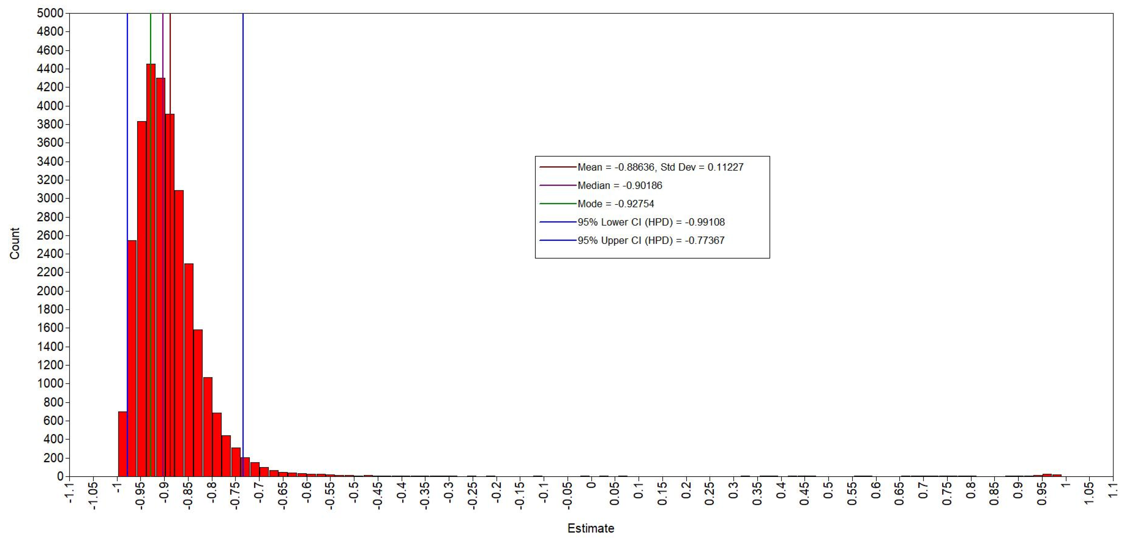
| H8a | Scope3 CO₂e → Pr_Mrg | 14,000 | 1.000 | −0.886 | 0.112 | 0.003 | −0.991 | −0.774 | ** |
| H8b | Scope3 CO₂e → EBITDA_Mrg | 22,500 | 1.000 | −0.733 | 0.554 | 0.111 | −0.995 | 0.914 | |
| H8c | Scope3 CO₂e → Op_Mrg | 29,300 | 1.048 | −0.266 | 0.855 | 0.357 | −0.985 | 0.960 | * |
| Direct and Indirect | |||||||||
| H9a | [Scope 1 + 2 CO₂e] → Pr_Mrg | 11,700 | 1.000 | −0.050 | 0.033 | 0.059 | −0.115 | 0.014 | |
| H9b | [Scope 1 + 2 CO₂e] → EBITDA_Mrg | 9900 | 1.000 | −0.060 | 0.035 | 0.042 | −0.130 | 0.009 | |
| H9c | [Scope 1 + 2 CO₂e] → Op_Mrg | 13,700 | 1.000 | −0.034 | 0.031 | 0.135 | −0.096 | 0.026 | |
| Corporate Value Chain | |||||||||
| H10a | [Scope 1 + 2+3 CO₂e] → Pr_Mrg | 14,700 | 1.000 | −0.050 | 0.032 | 0.056 | −0.116 | 0.012 | |
| H10b | [Scope 1 + 2+3 CO₂e] → EBITDA_Mrg | 18,100 | 1.001 | −0.060 | 0.035 | 0.042 | −0.130 | 0.008 | |
| H10c | [Scope 1 + 2+3 CO₂e] → Op_Mrg | 11,500 | 1.000 | −0.034 | 0.031 | 0.133 | −0.093 | 0.028 | |
Disclaimer/Publisher’s Note: The statements, opinions and data contained in all publications are solely those of the individual author(s) and contributor(s) and not of MDPI and/or the editor(s). MDPI and/or the editor(s) disclaim responsibility for any injury to people or property resulting from any ideas, methods, instructions or products referred to in the content. |
© 2023 by the authors. Licensee MDPI, Basel, Switzerland. This article is an open access article distributed under the terms and conditions of the Creative Commons Attribution (CC BY) license (https://creativecommons.org/licenses/by/4.0/).
Share and Cite
Porles-Ochoa, F.; Guevara, R. Moderation of Clean Energy Innovation in the Relationship between the Carbon Footprint and Profits in CO₂e-Intensive Firms: A Quantitative Longitudinal Study. Sustainability 2023, 15, 10326. https://doi.org/10.3390/su151310326
Porles-Ochoa F, Guevara R. Moderation of Clean Energy Innovation in the Relationship between the Carbon Footprint and Profits in CO₂e-Intensive Firms: A Quantitative Longitudinal Study. Sustainability. 2023; 15(13):10326. https://doi.org/10.3390/su151310326
Chicago/Turabian StylePorles-Ochoa, Francisco, and Ruben Guevara. 2023. "Moderation of Clean Energy Innovation in the Relationship between the Carbon Footprint and Profits in CO₂e-Intensive Firms: A Quantitative Longitudinal Study" Sustainability 15, no. 13: 10326. https://doi.org/10.3390/su151310326
APA StylePorles-Ochoa, F., & Guevara, R. (2023). Moderation of Clean Energy Innovation in the Relationship between the Carbon Footprint and Profits in CO₂e-Intensive Firms: A Quantitative Longitudinal Study. Sustainability, 15(13), 10326. https://doi.org/10.3390/su151310326