1. Introduction
Cycling offers numerous societal benefits and has an impact on safety, the economy, the environment, equity and health [
1,
2,
3,
4,
5,
6,
7,
8]. However, the popularity of cycling as a mode of transportation varies significantly between countries [
9]. The number of cyclists on the streets is highly influenced by their perception of safety [
2], making it essential to establish a clear metric for identifying and comparing risk factors related to road safety. Moreover, bicycle accidents, particularly less severe incidents, are often underreported [
10,
11,
12,
13,
14]. To pursue the Zero Vision goal [
15,
16], an approach focused on cyclists’ risk perception is suggested.
Promoting cycling safety increases the number of cyclists on the streets, resulting in safety in numbers and improved overall safety for all road users [
2]. Cycling and walking offer economic benefits for individuals, companies and communities [
3] and contribute to reducing dependency on non-renewable energy sources, thereby lowering greenhouse gas emissions [
17]. Moreover, cycling encourages equity by providing a more affordable transportation option for low-income families [
5,
6] and promotes physical and mental health by fostering a less sedentary lifestyle [
3]. By prioritizing cyclist safety, societies can enjoy many benefits, such as safer roads, decreased congestion and overall enhancements in public health and well-being.
During the COVID-19 pandemic, governments promoted cycling as an alternative to driving or crowded public transport [
18]. More polluted areas, where it may be hard to ensure social distancing, pose an additional risk of infection to their inhabitants and on public transport. For these reasons, the United Kingdom (UK) government is boosting this form of sustainable transportation with a package of GBP 2 billion [
19]. Public mobility patterns have undergone significant changes since 2020. The impact of the pandemic on people’s way of life has not yet been fully understood [
20], but there is a window of opportunity for safer and more environmentally friendly cities [
18] with a demand to understand cyclists’ risk factors. In the past, research studies were performed generally looking at city safety. In 2014, the analysis of color distribution in images, using color histograms, played a key role in predicting perceived safety in neighborhoods [
21]. Later, in 2016, convolution neural networks were first employed with the same general objective—rating neighborhood safety [
22].
The main objective of this research study is to create a scalable, robust and inexpensive solution to detect the areas of high perceived risk for cycling in urban areas. This was made possible by using state-of-the-art applications in computer vision (CV) and deep learning (DL) and the image database in Google Street View (GSV), which is publicly available and covers most developed countries [
23]. For this reason, this is a cost-effective approach to analyze city environments. Thus, large datasets and state-of-the-art models are used for object detection (OD) [
24] and image segmentation (IS) [
25] to achieve accurate results.
This project aimed at harnessing the power of AI to create safer urban environments for cyclists. The initial objective focused on identifying the most relevant risk factors affecting cyclists, considering safety metrics such as accident, injury and fatality rates. A GSV image dataset from Greater London was employed to extract these risk factors using OD and IS methods. The study examined the distribution of safety factors across London’s Lower Layer Super Output Areas (LSOA), aiming to identify correlations among frequently detected objects. LSOAs are geographic areas used for the collection and publication of small area statistics, comprising between 400 and 1200 households with a usually resident population between 1000 and 3000 persons in London [
26]. Additionally, the research aimed to pinpoint the most common misclassifications made by both algorithms and suggest methods for addressing them. Ultimately, the project sought to develop new guidelines on using OD and IS models to detect road safety risk factors.
This article is structured as follows. The Background section introduces road safety indicators and then discusses cyclists’ risk factors and explains how they are captured using OD and IS algorithms. Details are provided on the YOLOv5 (OD) and PSPNet101 (IS) models and the respective datasets used to train them. The Methodology section elaborates on handling and processing the GSV imagery dataset using the YOLOv5 and PSPNet101 models, selecting relevant parameters and the software and hardware utilized for execution. Lastly, the Results section offers an overview of the GSV imagery dataset across all London LSOAs and presents the outputs of the OD and IS trained models.
2. Background
2.1. Computer Vision and Deep Learning
Computer vision, a rapidly growing field in computing, focuses on teaching computers to perceive and comprehend visual information, such as images and videos [
27]. The goal is to replicate human vision. Deep learning, a branch of artificial intelligence, employs multi-layered neural networks to automatically identify representations required for detection or classification, enabling machines to learn complex functions from raw data. Similarly, DL has improved the state of the art in domains such as speech recognition, visual object recognition and object detection [
28]. However, disadvantages include dependence on the quantity and quality of input data, computational costs and interpretability issues [
29,
30].
2.2. Road Safety Indicators
Road safety indicators are essential for policymaking. According to the European Road Safety Charter [
31], they help assess the current situation of the roads, assess the impact on accident rates after an intervention, monitor progress over time and predict further evolutions. According to the European Road Safety Charter [
31], road safety indicators should comply with several criteria:
- (a)
Relate to specific aspects of road safety, such as the causes or consequences of a road accident;
- (b)
Be measurable in a reliable way;
- (c)
Be monitorable over time;
- (d)
Allow road safety engineers or public health experts to set targets;
- (e)
Help establish comparisons and benchmark different safety performances.
Six criteria are common to all indicators: geographical scope, timespan, numerical format, representation/visualization, reliability/accuracy/representativeness and a specific level of road safety. Geographical scope refers to the area where the measurement is taken, such as an organization, city, region, country, continent or the world. Timespan concerns the time frame the analysis covers, ranging from a day to a decade or longer. The numerical format involves the units of measurement, which can be proportions, percentages or other well-defined ratios.
Visualization denotes how data is presented using maps, graphs or tables, while reliability, accuracy and representativeness are connected to the design and implementation of the measurement system. The level of the indicator varies based on its focus, which can include crash impacts, post-crash responses, crash outcomes, crash causes and predictors, road safety policy and measures, or safety culture and safety systems.
In determining the risk factors discussed in the subsequent section, crash outcomes like mortality, injury severity and accident rates were considered. Moreover, road safety indicators were employed to rank the most relevant risk factors for cyclists. This comprehensive approach allows for a deeper understanding of the factors influencing cyclists’ safety and helps inform targeted interventions.
2.3. Perceived Risks
Various factors discourage people from cycling, such as perceived crash risks, weather conditions and lack of safety. Studies have shown that non-habitual cyclists are more prone to accidents, influencing their risk perception based on negative experiences [
32,
33]. Perceived risks are barriers to taking up cycling and must be addressed to create people-centered cities [
33,
34]. A bicycle should be regarded as a safe mode of transport to encourage its use.
Cyclists’ risk perception is influenced by accidents or near misses, particularly among potential or occasional cyclists [
33,
35,
36]. While cycling accidents are relatively rare and often underreported, events perceived as risky are more frequent. Therefore, reducing risky incidents is a more effective approach to avoiding crashes. This involves heeding “early warnings” to prevent severe situations that may result in hospitalizations. However, quantifying events that do not lead to accidents is challenging. Initiatives like PING [
37] have emerged, allowing cyclists to report perceived risk situations by pressing a button on a device attached to their bicycle’s handlebars. This crowdsourcing process generates high-quality georeferenced data on the risks perceived by cyclists.
The approach proposed in this study differs because it achieves scalability and permeability within the city. By using DL techniques, areas with high perceived risk for cyclists were identified. By leveraging advanced techniques like object detection and image segmentation, it is possible to understand the factors contributing to road safety and inform interventions promoting cycling as a secure and appealing transport option.
2.4. Risk Factors (Based on London LSOA Data)
To list and order the most relevant risk factors for cyclists, accident, injury and fatality rates were considered. In London, the annual fatality rate for cyclists is relatively low, ranging from sixteen in 2011 to eight in 2016 [
38]. Consequently, accident and injury rates were used to order all risk factors when designing the diagram presented in
Figure 1. A strong qualitative and experience-based component was also inherent to these rankings since a common safety metric for all risk factors was not found. The top three most relevant factors that influence cyclists’ safety are the presence or lack of a cycle lane, road speed limits and lane width. Statistical data that support the rankings defined in
Figure 1 have been provided, but few accidents involving cyclists are reported [
10,
11,
12,
13,
14].
Considering
Figure 1, the number of risk factors decreases from left to right in the diagram. The most unsafe situation was the absence of a cycle lane, followed by high speed limits with a narrow lane in an on-road scenario, high speed limits but with a wider lane and low speed limits regardless of the presence of a narrow or wide on-road lane. A physically separated cycle lane was considered the safest scenario.
2.4.1. Cycle Lane
Cycle lanes can be classified into two categories: physically separated lanes and on-road lanes. Physically separated lanes reduce the probability of a crash, especially when a car tries to overtake a cyclist, or of hitting a cyclist if they fall off. When there are no vehicles parked nearby, these lanes reduce the risk of injury among cyclists by half [
39]. Furthermore, opening a car door poses a significant threat to bicycle riders [
40]. For all these reasons, risks associated with high speed limits, narrow bicycle lane widths, road pavement quality and parked cars were not considered.
In the case of on-road cycle lanes, vehicle speeds tend to be lower, and there are fewer interactions between vehicles and the cyclists compared to when there is no separate lane [
41]. This makes the physically separate cycle lane the safest scenario, followed by on-road lanes and no cycle lane at all. Finally, having a cycle lane was considered the most decisive factor in preventing many previously identified risks. It was considered number one in the rankings of risk factors.
2.4.2. Vehicle Speed
Vehicle speed was one of the major factors involved in around 10% of all accidents and 30% of fatalities. The speed of vehicles involved in a crash is the most critical factor in determining the severity of injuries [
42,
43]. There are two distinct factors when considering speed. Not only are higher speeds known to be responsible for a higher rate of accidents, injuries and deaths but so too are significant speed variations. Roads with many speed variations are more unpredictable as they favor a higher number of interactions and an increased number of overtaking maneuvers. Consequently, sometimes reducing speed limits may only decrease the vehicles’ average speed and not its variation in speed as it accelerates and brakes [
44]. The crux of the danger posed by high speeds is the increase in the braking distance and kinetic energy transferred from the vehicle to the cyclist. As both increase by the square of velocity, the possibility of avoiding or surviving a crash decreases quadratically [
44].
From a biological perspective, the human body can only resist a limited amount of kinetic energy transfer in a crash [
45]. This varies for different body parts, age groups and genders. Considering the most well-designed car, this limit can be exceeded if the vehicle exceeds 30 km/h [
16]. Studies also show that if a car travels at less than 30 km/h, a pedestrian’s probability of surviving a crash is higher than 90%. When hit by a car at 45 km/h, the chance of surviving decreases to 50% [
46]. Conclusively, this was considered the second most relevant factor in cyclist safety. For an on-road cycle lane on a road with a low speed limit, the risk factors related to parallel traffic were considered negligible, regardless of the lane width.
2.4.3. Lane Width
In the United Kingdom, the recommended cycle lane width is 2.0 m (one way). The minimum requirement is 1.5 m, while cycle tracks accommodating two-way cycling should be 2.5 m wide. All values below 1.5 m are considered too narrow, allowing too little space to maneuver around obstacles, such as debris, potholes and drains. After the road speed limits, cycle lane width was considered the most important factor. Whenever it is considered wide, traffic risk factors were not considered. Regardless of the width of an on-road cycle lane, low speed limits were enough to rule out traffic-related risk factors.
2.4.4. Street Lighting
Street lighting was considered the next most relevant criterion for road safety. It affects drivers’ and cyclists’ reaction time, and a lack of lighting makes cyclists difficult to notice, especially when they are not using any reflective or luminous gear. Moreover, from the cyclists’ perspective, poor lighting means they are less aware of other road risks, such as pavement quality.
2.4.5. Pavement Quality, Tram/Train Rails and Water Drainers
As frequently referred to in the literature, pavement quality is crucial when evaluating safety [
47,
48,
49]. It refers to the quality of the road when there is no cycle lane or of the cycle lane itself when there is one. Pavement defects, including potholes, along with water drainers and tram/train rails, contribute to an increased number of falls among bicycle riders. The impact of these factors decreases when street lighting is improved and when cycling is performed within the speed limit of 25 km/h.
2.4.6. Number of Intersections and Intersection Visibility
Intersections are naturally areas of interaction between different road users. Therefore, the majority of bike and car crashes occur at intersections. Asgarzadeh et al. [
50] reported that 60% of total crashes happen at intersections. Additionally, as part of the same study, intersections where streets do not meet at right angles posed an additional danger to cyclists. Crashes in these areas were 31% more likely to cause serious injury to cyclists due to the lack of visibility.
2.4.7. Lorries and Other Large Vehicles
Economic development and consumer demand have increased in recent years and so has the number of trucks inside cities [
51,
52]. Cycling has followed the same trend, so the number of encounters between cyclists and trucks has significantly increased. For example, 15% of the bicycle lane network in New York City overlaps with 11% of the truck road network [
53]. The increased encounters have contributed to higher accident and mortality rates involving trucks.
Truck–bicycle accidents usually have more severe consequences than any other type of accident [
54,
55,
56,
57]. In some European countries, 30% of all cycling fatalities are associated with trucks [
58]. In the past two decades, studies have identified trucks as the most common vehicle category in London’s cyclist deaths [
55,
59,
60].
2.4.8. Advanced Stop Line
Advanced stop lines exist in several European countries, such as Belgium, Denmark and the United Kingdom, and they give a head start to certain types of vehicles (namely, bicycles) when the traffic signal changes from red to green. This has several advantages. First, drivers behind the line will be more aware of cyclists around them and take the proper precautions to avoid dangerous maneuvers. Second, it becomes safer for cyclists to turn left, avoiding crashes with cars behind them. A schematic layout can be seen in
Figure 2.
2.4.9. Bend Visibility
Several sources identify bends as a risk factor. Bends and intersections are often jointly considered as they pose similar risks to the cyclist. From the cyclist’s perspective, low visibility when cycling around bends makes usually low-risk situations, such as the sudden presence of pedestrians or invasive vegetation, more dangerous. Poor visibility can make cyclists unnoticeable and vulnerable to drivers [
47].
2.4.10. Pedestrians
In the USA, among all age groups, pedestrian fatalities most often occur in children younger than 14 years old, compared with adults aged between 15 and 64 or 65 or more. Regarding of gender, men are at a greater risk than women [
62]. For these reasons, locations with a higher concentration of people satisfying these criteria (e.g., school areas) are at additional risk. Nevertheless, accidents between pedestrians and cyclists in car-free zones are rare and seldom serious [
63]. Thus, pedestrian density was considered the least important of the risk factors.
3. Tools Used to Capture Objects and Structures from Imagery Dataset
3.1. Object Detection Using YOLOv5
Object Detection is a computer technology associated with image processing and CV and used in applications like image annotation, activity recognition and face detection [
64]. Objects have specific features that help classify them into distinct classes. OD methods can be divided into machine-learning-based or deep-learning-based approaches. Machine learning approaches, such as support vector machines, require a predefined list of relevant features, while deep learning approaches, like Convolution Neural Networks, perform end-to-end OD without specifying these features [
64].
YOLOv5, a deep learning approach, operates within the PyTorch framework [
24]. Its architecture consists of three essential parts: the model backbone, neck and head. These are responsible for extracting features, obtaining feature pyramids and generating output vectors, respectively. Cross stage partial networks, used in version 5, have significantly improved processing time with deeper networks. The model’s head applies anchor boxes on features and generates output vectors, including class probabilities and bounding boxes, with each potential detection having an associated confidence score.
Due to the high accuracy and speed of YOLOv5x (see specifications in
Table 1), this model was chosen to process the images.
Table 1 showcases the specifications of the YOLOv5x model, considered the most accurate among the various YOLOv5 implementations. The table comprises several essential metrics to assess the model’s performance. Average precision (AP), a common metric in object detection, is provided for both validation (AP
val) and test (AP
test) datasets. AP
50 signifies the average precision at a 50% overlap threshold between the predicted and ground truth bounding boxes. The model’s processing speed on a GPU (Speed
GPU) is expressed in milliseconds per image. FPS
GPU indicates the number of frames processed per second on a GPU, reflecting the model’s real-time performance. The Params column denotes the total number of parameters in the YOLOv5x model, while the Weights Size (MB) column displays the size of the model’s weights file in megabytes.
3.2. Image Segmentation Using PSPNet101
In CV and image processing, image segmentation (IS) is the partitioning of a digital image into multiple segments or pixels. The goal is to simplify image representation to the point that multiple structures can be easily retrieved. More precisely, IS assigns a label to every pixel in an image, and the ones with the same label share characteristics. Consequently, this method provides information on the presence of certain structures, shape and location in the image [
65].
The pyramid scene parsing network (PSPNet) is one of the most accurate IS models. It won the ImageNet Scene Parsing Challenge 2016, PASCAL VOC 2012 and Cityscapes benchmarks. It achieved a mean intersection over union (mIoU) accuracy of 85.4% on PASCAL VOC 2012 and 80.2% on Cityscapes [
25]. In the past two years, its segmentation model accuracy has reached a plateau. Similarly, after 2017, the increase in the mIoU has been minimal [
66].
After receiving an input image, PSPNet executes a convolutional neural network (CNN) to extract a feature map from the last convolutional layer. Then, a pyramid parsing module is used to harvest different sub-region representations, followed by upsampling and concatenation layers to create the final feature representation. This carries both local and global context information. The representation is fed into a convolution layer and the final per-pixel prediction is obtained in the last step.
3.3. Training Datasets
Several datasets exist that contain labeled objects and segmented images. For object detection (OD) model training and benchmarking, MS Coco [
67] and Open Images V6 [
68] are two widely used datasets with a high number of road categories. For image segmentation (IS), Cityscapes [
69] and ADE20K [
70] represent the current state-of-the-art datasets.
Table 2 compares these four datasets based on their relevant categories for assessing cyclists’ road safety. Some road safety objects can be extracted directly, while others require an indirect approach. The same applies to segmented structures.
A direct or indirect method was used to identify each risk factor in the images. Within the OD category, the following cyclist risk factors were identified: cars and parking meters for parked cars; people for pedestrians; trucks and buses for truck circulation; bicycles for the number of cyclists; traffic lights and stop signs for vehicle speed as they serve as traffic calming factors; and trains for the presence of tram/train rails due to their close association. Roads, sidewalks and streetlights were used for the IS category to obtain road and sidewalk widths and streetlighting.
3.3.1. MS Coco
Microsoft Coco is one of the biggest and most popular datasets used for OD, segmentation and captioning. It contains 330 K images, with 200 K that are labeled, and features 1.5 M labeled objects across 80 categories.
Figure 3 provides examples of labeled objects. The dataset includes several classes of everyday objects, from home appliances to those commonly seen on roads [
67]. In the image below, annotated objects are highlighted in color (top), and a list of the objects annotated in the image is also displayed (bottom).
3.3.2. Cityscapes
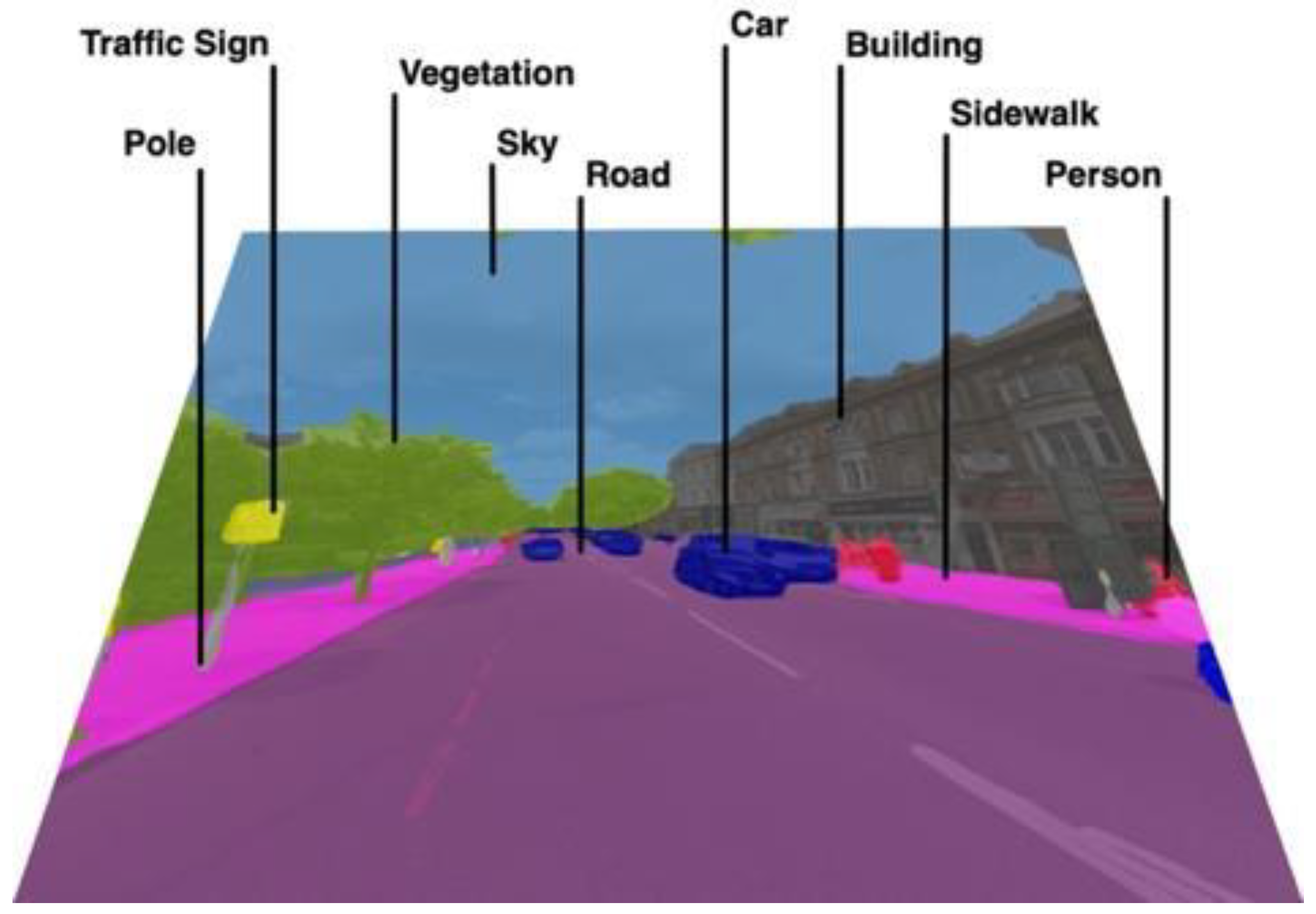
The Cityscapes dataset focuses on the semantic understanding of urban street scenes. It contains 20,000 coarsely annotated images and 5000 finely annotated images from 50 German, French and Swiss cities. These were captured over several months (summer, spring and fall) in good or medium weather conditions during daytime, and the dataset features 30 classes of structures (
Figure 4) [
69]. The image segments divide class structures into three different city environments.
Finally, MS Coco and Cityscapes datasets are the most complementary and contain the most relevant objects and road structures. Based on these two datasets, pre-trained YOLOv5x and PSPNet101 models were employed to detect objects and segment images, respectively.
4. Materials and Methods
4.1. GSV Imagery Dataset
Instead of considering a road safety analysis of London, we chose to perform it at an LSOA level. Greater London can be divided into smaller areas: output area, Middle Layer Super Output Area and LSOA. Each one of these subdivisions of London differs on a geographical scale. A zip folder containing multiple shapefiles for each division was obtained from London Datastore (data.london.gov.uk/dataset/statistical-gis-boundary-files-london accessed on 18 May 2020). The GSV imagery dataset was obtained using Street View Static API and the respective geographical coordinates. A separate file associating each image identification to a given London LSOA was produced using LSOA Atlas from Greater London Authority [
71]. Due to the high memory requirements, all images used in this project were stored in the Imperial College London servers.
The GSV dataset contains 518,350 images from Greater London, with 512,812 identified with a London LSOA. Of those, 478,724 are unique (
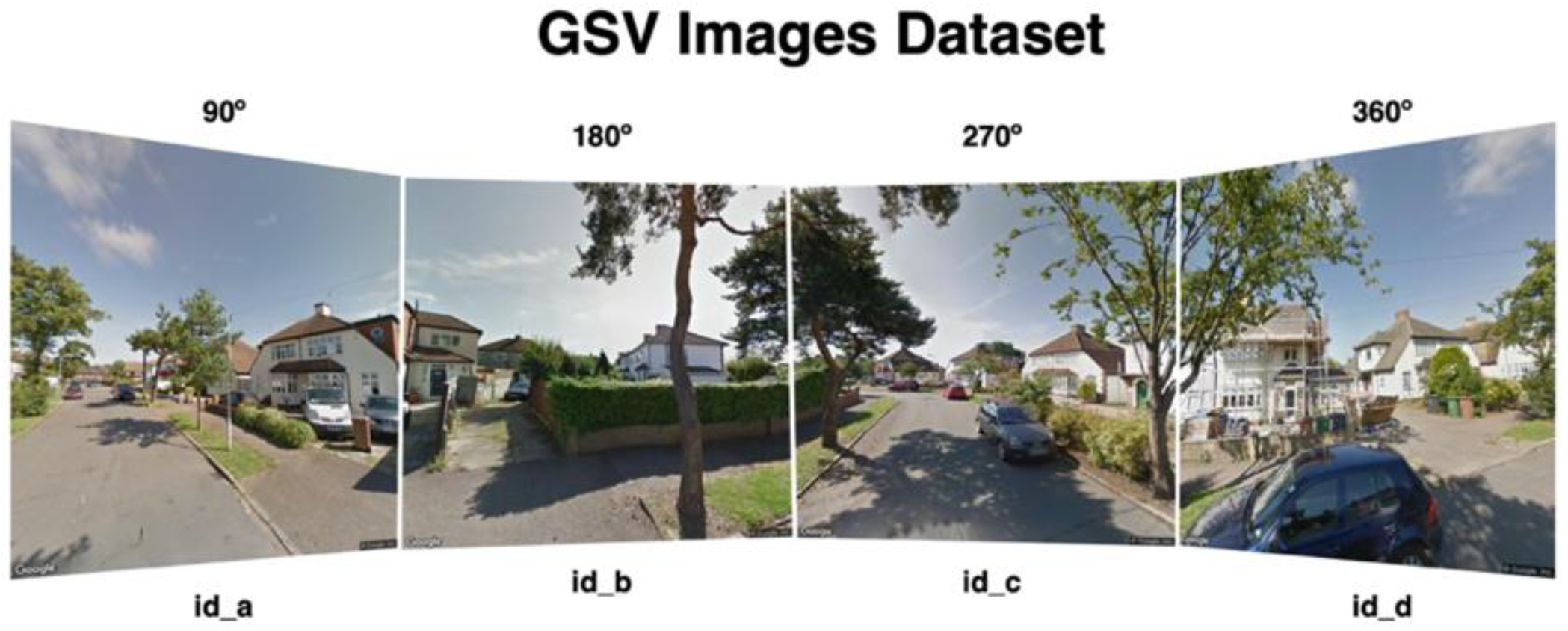
Table 3). Each datapoint has four images available, covering 0 to 360 degrees. There are 119,681 unique LSOA identified points, each with four 90-degree images (
Figure 5). There are more images available near Central London, and this number decreases as you move out to the periphery. In
Figure 6, an LSOA Atlas is shown, along with the respective geographical distribution of all images. The LSOA with the highest number of datapoints, 211, is in Central London. On average, 27 datapoints are available per LSOA, with one LSOA in the dataset having only one datapoint (
Table 4). The wide distribution of images compromises the accuracy of estimating the number of objects and segmented structures in less-well-represented LSOAs.
4.2. YOLOv5
The imperial high-performance computing cluster was utilized to run YOLOv5. Due to the model’s fast execution, a single P1000 GPU was used. The implementation with the most accurate set of weights of YOLOv5 was chosen—YOLOv5x. Also, a minimum confidence of 0.5 was defined for each detection (higher than the standard value of 0.4). Only text files containing the detected objects and respective locations were saved. Each line includes a numerical designation for each object and the coordinates of the center of the detection box, along with two values for the width and height of the rectangle.
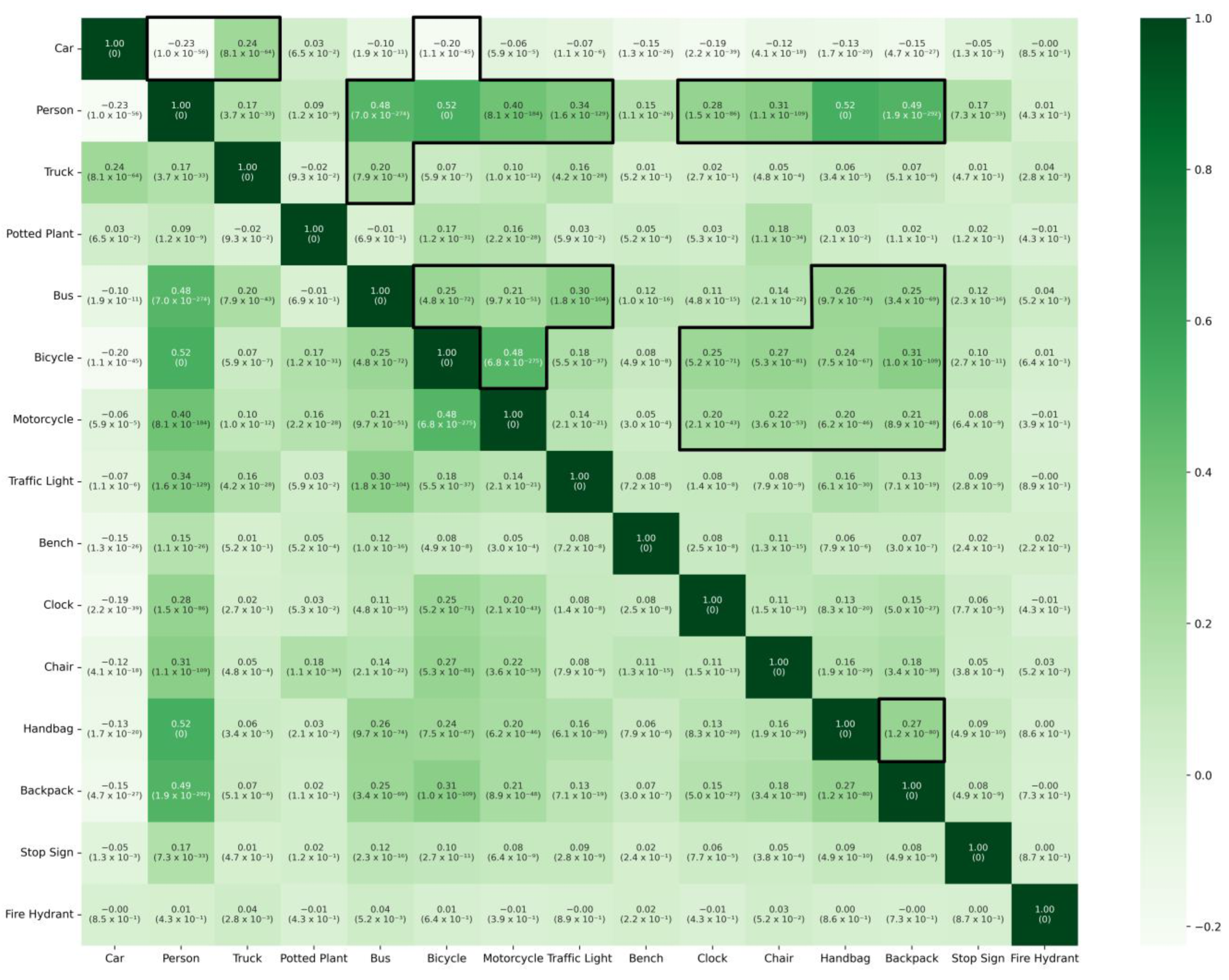
Python visualization frameworks Matplotlib and Seaborn were used to plot the correlation matrix for the top 15 most detected objects. Pearson correlation factors and
p-values were obtained using SciPy Pearson function (
Figure A3). Misclassifications, limitations and future directions analysis focused on the objects identified before as relevant for road safety. Moreover, all observations resulted from the individual assessment of one image from all London LSOAs and the overall project experience (
Figure A5).
4.3. PSPNet101
Although it was already available, a preliminary version of the implementation executing PSPNet101 was made, provided by Esra Suel. Modifications were made to overcome incompatibilities with the new version of TensorFlow. IS methods are generally slower than OD. Originally, the Python multiprocessing tool was used to accelerate execution. At the end, the original GSV dataset was split into 13 batches and executed parallelly in 13 P100 GPUs. Consequently, 13 jobs were submitted to the high-performance computing (HPC) cluster. P100 was the chosen GPU due to its higher processing power for numerical analysis (
Table 5). All images in the GSV dataset were segmented. After that, two Python functions were implemented: one that generates a dictionary linking each RGB color to a given object class and one that receives the full dataset of segmented images as input and outputs the total number of labeled pixels for each category. Relative and absolute distributions of all labels were analyzed and represented using Pandas DataFrame Python library. Misclassifications, limitations and future directions analysis focused on the structures identified before as relevant for road safety. Moreover, all observations resulted from the individual assessment of one image from all London LSOAs and the overall project experience (
Figure A6).
5. Results
5.1. Object Detection Using YOLOv5
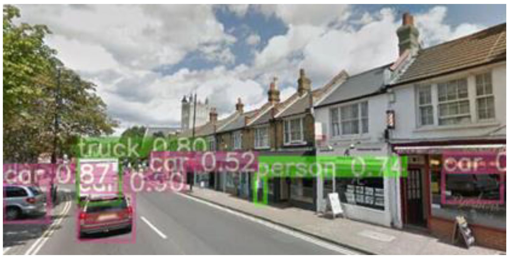
Figure 7 shows an example of image processing with YOLOv5. All cars, trucks and people in the image were accurately detected with high confidence values. All relative and absolute distributions of objects can be presented at a dataset level. As the dataset exclusively contains street view images, it was expected to detect a significant percentage of cars. London has a high population density and a large public transport system. This justifies the high number of pedestrians and buses that are detected. Potted plant detections are closely related to London’s number of parks and green areas.
Table 6 contains the absolute numbers of the top 15 most common objects detected in the GSV dataset. Highlighted in black are those identified as contributing positively to cyclists’ road safety. Grey ones are the negative risk factors. In addition to the risk factor objects in
Table 6, trains (657) and parking meters (968) were also considered to extract the risk factors in
Figure 1.
Figure 8 displays the distribution of objects relevant to identifying cyclists’ risk factors across different LSOAs. Bicycles are primarily detected in Central London as they are commonly used for short distances. There is also a higher concentration of buses in Central London, whereas trucks are found in greater numbers outside the city center due to the London Lorry Control Scheme restrictions. Both buses and trucks have long-tailed distributions, increasing the likelihood of unexpected events and putting cyclists at higher risk.
Car distribution is considerably denser outside Central London, where roads have more lanes, making it easier to detect cars. The reduced number of parking meters in the city center correlates with the lower presence of cars there. A significantly higher number of people are detected in the center, especially in the City of London and Westminster, which are the historical center and the central business district.
Stop signs and traffic lights are predominantly detected outside Central London, with their similar histogram distributions. However, the number of detected traffic lights is nearly five times greater than that of stop signs.
In the context of road safety, the strongest positive correlations include Person vs Bicycle (0.52), Person vs Bus (0.48), Bus vs Bicycle (0.25) and Bus vs Truck (0.20), while the strongest negative correlations are Person vs Car (−0.23) and Bicycle vs Car (−0.20) (
Figure A3). The high Person vs Bicycle correlation suggests pedestrians and cyclists feel safe sharing the same space. The relatively high Person vs Bus value is expected since buses are public transport, and many people are usually nearby.
A significant difference exists between Bicycle vs Bus and Bicycle vs Truck correlations, indicating that cyclists feel safer near buses than trucks. This is not surprising as bus drivers are more experienced with vulnerable pedestrians, and buses generally move slower than trucks. The relatively high correlation between buses and trucks, combined with their similar shapes, suggests they might sometimes be misclassified.
The statistically significant negative correlations of Person vs Car and Bicycle vs Car imply that areas with high car concentrations discourage cycling and walking. One factor that cannot be ruled out is the possibility of larger objects obscuring smaller ones, leading to a negative correlation. However, given the height at which the GSV images were captured, this is unlikely to be a frequent occurrence.
5.2. Image Segmentation Using PSPNet101
Figure 9 presents an example of a segmented image with labels for detected structures. Buildings (19%), the sky (15%), roads (15%), vegetation (12%) and cars (11%) account for 72% of the total area in all images. The prevalence of these structures is due to their inherent size, and since the dataset contains images from the streets of London, a higher number of cars is expected. Pixel frequency is related to object size and occurrence in images, and both OD and IS techniques seem consistent.
The relative distribution of segmented pixels across categories indicates that objects on the roads, as well as surrounding structures like buildings and the sky, can be detected. Some objects without a clear correlation to road safety also demonstrate the versatility of using GSV images for detecting structures in various locations. For example, 2750 clocks were misclassified as satellite dishes; 37,917 potted plants were identified in the building landscape; and 234 airplanes were detected in the sky.
Significant numbers of pixels labeled as sidewalks were detected, suggesting that regularly present objects are likely to be captured (e.g., 107,266 people, 5013 benches and 1168 fire hydrants).
Table 7 shows the absolute number of labeled pixels across nineteen segmented categories.
From an IS point of view, the GSV dataset appears to be useful for estimating roads and sidewalks due to the relatively high number of pixels detected and consistent shapes. The same applies to streetlights. Despite only 303 million pixels being identified, the dimensions of this object suggest that a significant number of those should have been detected. After individually analyzing one segmented image per LSOA for the complete dataset, it appears that both the area and shape of the streets and sidewalks can be accurately retrieved.
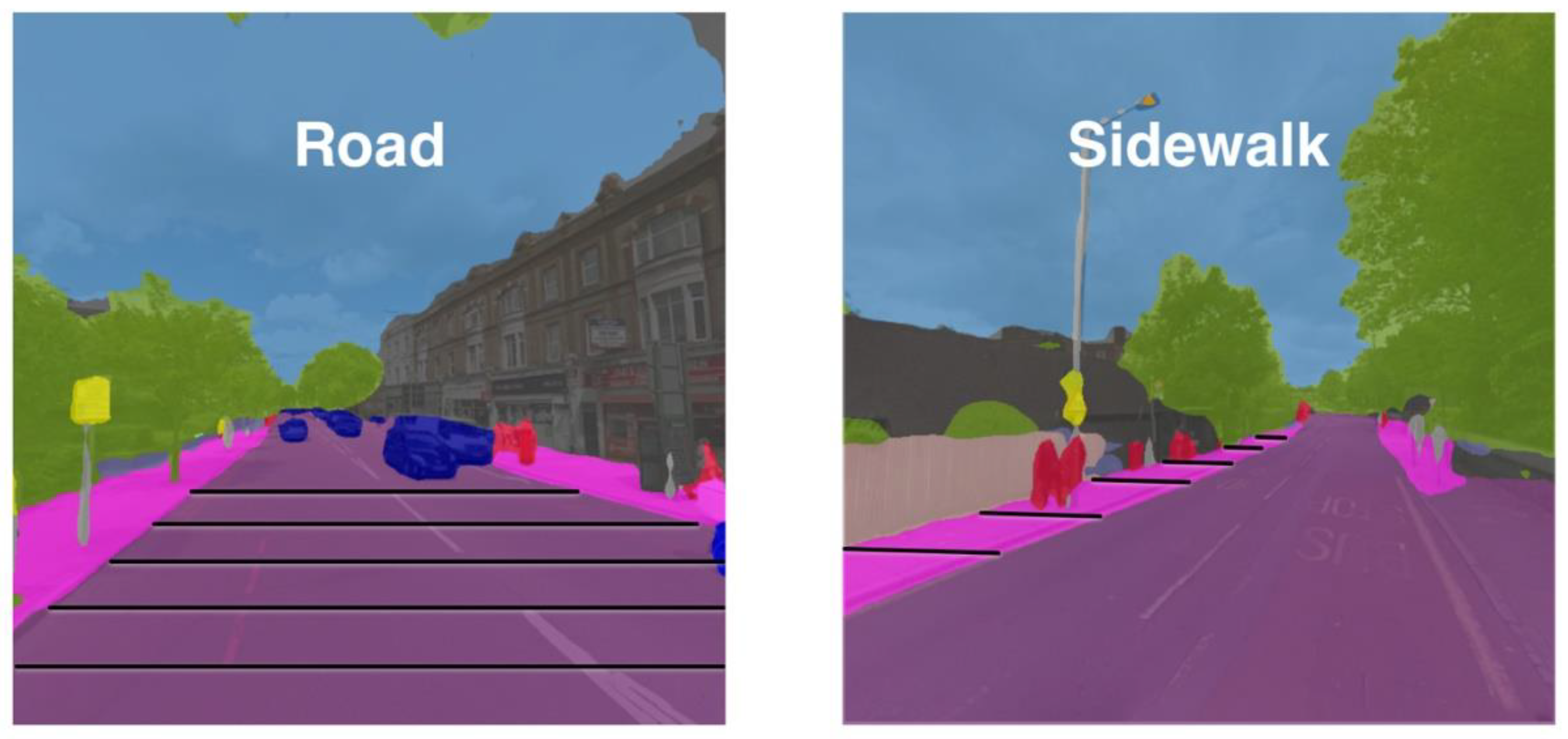
As the introduction states, these last properties are relevant in a road safety context because they allow us to calculate road and sidewalk width. Moreover, the presence of streetlights, or poles, as they are called in Cityscapes, is a proxy to assess road visibility. Therefore, in
Figure A4, these concepts are exemplified.
6. Limitations and Future Works
This study, focused on London, presents an investigation into deep learning techniques and GSV images for improving cycling safety. However, it is important to note that our study does not aim to develop AI-assisted cycling. Instead, we strive to provide risk information for cyclists, decision-makers and other stakeholders. Despite these contributions, we must acknowledge several limitations in our research.
One limitation is the generalizability of our results as they may not extend well to other cities or different urban environments with varying road safety regulations. Another limitation concerns the use of GSV. While this approach offers an efficient method for image analysis, it comes with its own set of limitations, such as coverage issues and the existence of outdated images.
Furthermore, the GSV images used in our study vary in time, day, week and year. Therefore, important variations in the objects present may not be accurately evaluated. As elements in images can overlap, this can also affect the accuracy of our metrics on those images.
Similarly, the risk factors considered in this study were limited to those that could be extracted from the images in the London urban context. Important factors such as weather conditions, traffic volume and others were not considered. The employed object detection and image segmentation techniques also present limitations. These methods might not capture all relevant objects or accurately segment them from the images, leading to potential inaccuracies in the analysis. This will be discussed in more detail in the following subchapters.
6.1. Object Detection Using YOLOv5
A precise metric was not found to estimate cyclists’ road safety based on the detected objects on the roads. However, based on the objects’ distributions in
Table 6, one positive safety measure and another negative safety measure combined with it were formulated.
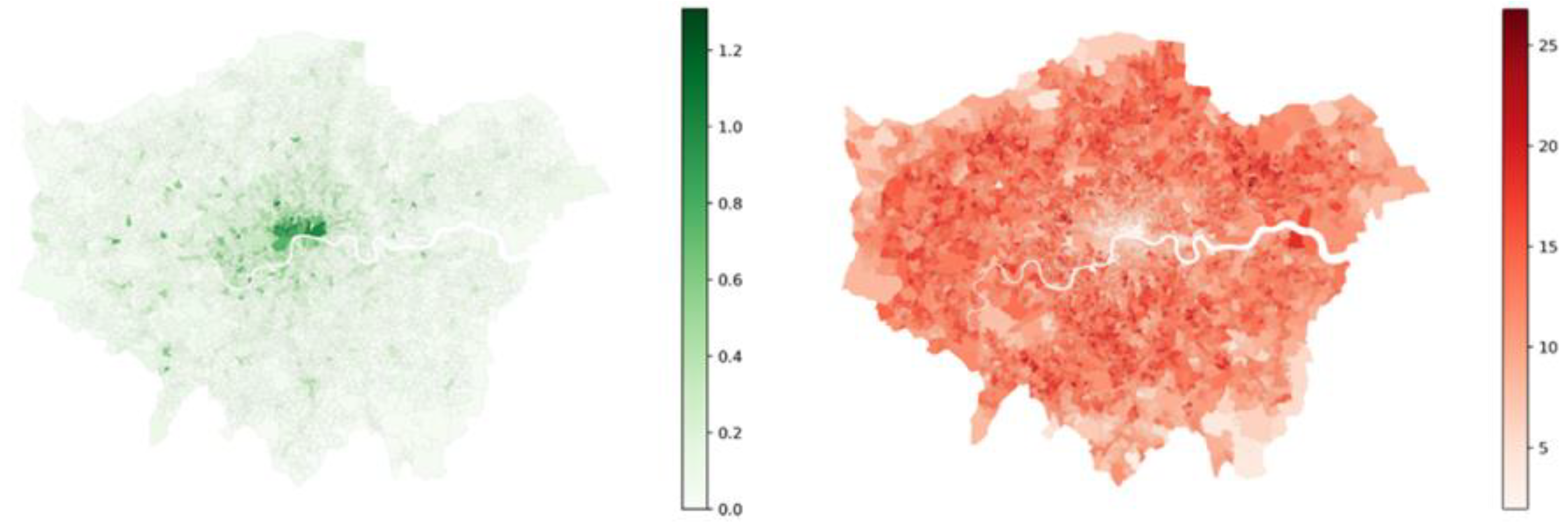
One feature that influences cyclists’ safety is the number of other cyclists in the surrounding area. This happens because drivers become more aware of their presence when in larger numbers. Moreover, most serious injuries are caused by crashes between vehicles and cyclists. It was found that there is a statistically significant negative correlation between the presence of cars and people. Thereafter, the higher the presence of pedestrians, the lower the number of cars. Consequently, there is less of a risk for cyclists to be injured. Bicycle and Person LSOAs were combined into one, after calculating the average number of these objects per image. If cars are the main contributors to injury rates, heavy vehicles are particularly relevant when analyzing fatality rates. A second LSOA map was created joining the average number per image of the following objects: Bus, Car, and Truck.
It is important to highlight that we cannot extract a holistic safety metric from these two generated LSOAs (
Figure 10). A simple example is a road where cyclists are physically isolated from the traffic, which is not necessarily unsafe for cycling.
A high level of confidence was found for all the detected road safety objects. YOLOv5 can detect a wide range of object sizes, even when partially occluded (
Figure A5). Moreover, low contrast between objects and background does not appear to have caused a high number of non-detections. An example of this was when the algorithm detected a car reflected in a window on the streets of London. Nevertheless, this is considered a misclassification. A set of ten random object detected images was compiled so that the readers can verify the accuracy of YOLOv5 (
Figure A5) by themselves. The results are driven by GSV images, so characteristics like traffic and time of day will vary depending on that source.
6.2. Image Segmentation Using PSPNet101
Due to the dimensions of specific structures, PSPNet101 could not accurately capture their shape. One example is a thin pole. The resolution of the images in the dataset highly influences their detection. This is not particularly problematic since the most important thing about these structures is their detection and not their shape. In terms of the streets and sidewalks, occlusion is sometimes an issue.
Nevertheless, accounting for the objects usually present in any of these areas, considering their overlapping areas simultaneously seems to be an effective workaround. This was particularly observed for cars on the roads and people on the sidewalks. In this way, it should still be possible to extract information on the shape and size of these structures. Extracting the absolute dimensions of these structures on the streets of London can be a challenging task. Criteria can widely vary according to the angle at which the images were taken. One way to overcome this would be to focus on the relative dimensions across the objects (
Figure A6).
6.3. Future Works
A possible future development for OD could involve training YOLOv5 with a larger dataset and with a higher number of object categories than MS Coco. This would involve annotating additional images. Documentation on how to train YOLOv5 is available in its GitHub repository. Static images cannot capture several features. Using video recordings, including pedestrian, cyclist and vehicle movement, would capture variables that are highly influenced by the time images obtained.
In terms of IS, retraining PSPNet101 with more images and classes will increase its accuracy. Moreover, using the information on the dimensions and shape of the different structures will also help estimate road safety.
Finding a metric that automatically accounts for the presence of different objects and structures will make cycling safety estimation a more analytical process. This can be achieved by crowdsourcing many road images and asking users to rate individually or choose the safest of two images. After identifying objects and structures in the same dataset, a neural network can be trained to approximate a function that automatically predicts a safety score for an image.
In addition to refining the OD and IS models, another important future direction is the possibility of developing a routing system that avoids points where cyclist risk factors are detected. This would involve utilizing the outputs of the OD and IS systems to inform decisions on route planning for cyclists. Moreover, these outputs could alert authorities to locations requiring corrective maintenance, thereby potentially mitigating these risk factors. Alternatively, these risk factor notifications could be directly conveyed to users via a mobile application, road signs or awareness initiatives.
Future directions of research on this topic include increasing the availability and resolution of GSV images; training YOLOv5 and PSPNet101 with datasets containing a higher number of categories relevant for road safety; defining a safety metric to weigh and combine, at road level, detected objects or segmented structures; and processing street view images or video in real time, which would mean we can better capture the dynamics of road safety.
7. Conclusions
This project aimed to extract cyclists’ road risk factors from Google Street View images of Greater London using object detection and image segmentation techniques. The study focused on image distribution across all Lower Layer Super Output Areas (LSOAs), identifying relevant road safety indicators and determining and ranking cyclists’ risk factors using YOLOv5 and PSPNet101 for object detection and image segmentation, respectively.
Approximately 2 million objects were identified, and 250 billion pixels were labeled in the 500,000 images available in the dataset, with an average of 108 images per LSOA. YOLOv5 detected the distribution of risk factors at the LSOA level. The number of cyclists and pedestrians was higher in Central London, while there was more traffic outside this area. Statistically significant negative correlations were observed between cars and buses, cars and cyclists, and cars and people, while positive correlations were noted between people and bicycles and people and buses. PSPNet101 identified building (19%), sky (15%) and road (15%) pixels as the most common, suggesting that objects in these areas can be detected equally.
The work presented marks an initial step towards increasing cyclist safety. In this study, we developed a comprehensive methodology to identify risk factors for cyclists. The recognition of these risk factors is a foundation for developing strategies to improve cycling safety. As a future course of action, it is necessary to create frameworks to communicate this information to end users and decision-makers effectively. This can facilitate implementing measures to reduce cyclist risk, promoting safer cycling environments.
In conclusion, this research highlights the potential of deep learning techniques in identifying and addressing cyclists’ risk factors in urban environments. By incorporating these techniques into urban planning and transportation management, we can create cities that prioritize the safety and comfort of all residents while reducing carbon emissions and mitigating climate change impacts. As we continue to harness the power of artificial intelligence, the research aims to develop safer, more sustainable cities that cater to the needs of cyclists, pedestrians and all road users. These initiatives align with broader sustainable development goals, promoting environmentally friendly and inclusive urban environments.
As the study moves forward, it will explore other areas where AI-driven solutions can further enhance city safety and sustainability. By focusing on continuous innovation and improvement, our team envisions a future where cities are safer, more livable, resilient and environmentally friendly. This study marks a promising beginning, and our team is committed to advancing its mission of harnessing artificial intelligence to create a better urban experience for everyone.
Author Contributions
Conceptualization, L.R., R.N. and M.P.; methodology, L.R. R.N., E.M. and A.B.M.; software, L.R.; validation, L.R., R.N., T.T. and A.F.; formal analysis, L.R. and T.-C.B.; investigation, L.R.; resources, L.R., R.N. and M.P.; data curation, L.R., T.-C.B., E.S., E.M. and A.B.M.; visualization, L.R., R.N., E.M. and T.T.; writing—original draft preparation, L.R., R.N., M.P., T.-C.B., E.M., T.T. and A.F.; writing—review and editing, T.T. and A.F.; supervision, R.N. and A.F.; project administration, R.N., M.P. and A.F.; funding acquisition, R.N. and A.F. All authors have read and agreed to the published version of the manuscript.
Funding
This research was funded by the Research Center for Territory, Transports and Environment-CITTA (UIDP/04427/2020) and by the Association for the Development of Civil Engineering (ACIV).
Institutional Review Board Statement
Not applicable.
Informed Consent Statement
Not applicable.
Data Availability Statement
All results, data and implementations were made available in the project’s repository (github.com/luisdrita/RoadSafety updated on 3 Setember 2020) accessed date 10 June 2023.
Acknowledgments
We are deeply grateful to the MRes Biomedical Research (Data Science) supervisors of L.R., Majid Ezzati and Ricky Nathvani, and all other people from Imperial’s School of Public Health, including Barbara Metzler, Emily Muller, Esra Suel and Theo Rashid. We also thank Kavi Bhalla (University of Chicago), Jill Baumgartner (McGill University) and Michael Brauer (University of British Columbia), who had important contributions to this research project, and all the CycleAI former team members, Stamatios Kourkoutas, Gonçalo Moreno and Francisco Pereira, who made this project meaningful and a once-in-a-lifetime experience.
Conflicts of Interest
The funders had no role in the study; in the collection, analyses or interpretation of data; in the writing of the manuscript; or in the decision to publish the results.
Appendix A. YOLOv5 Detected Objects
One of the main goals of this project was to show the potential of the GSV imagery dataset. Given a large dataset, there is plenty of information that can be extracted.
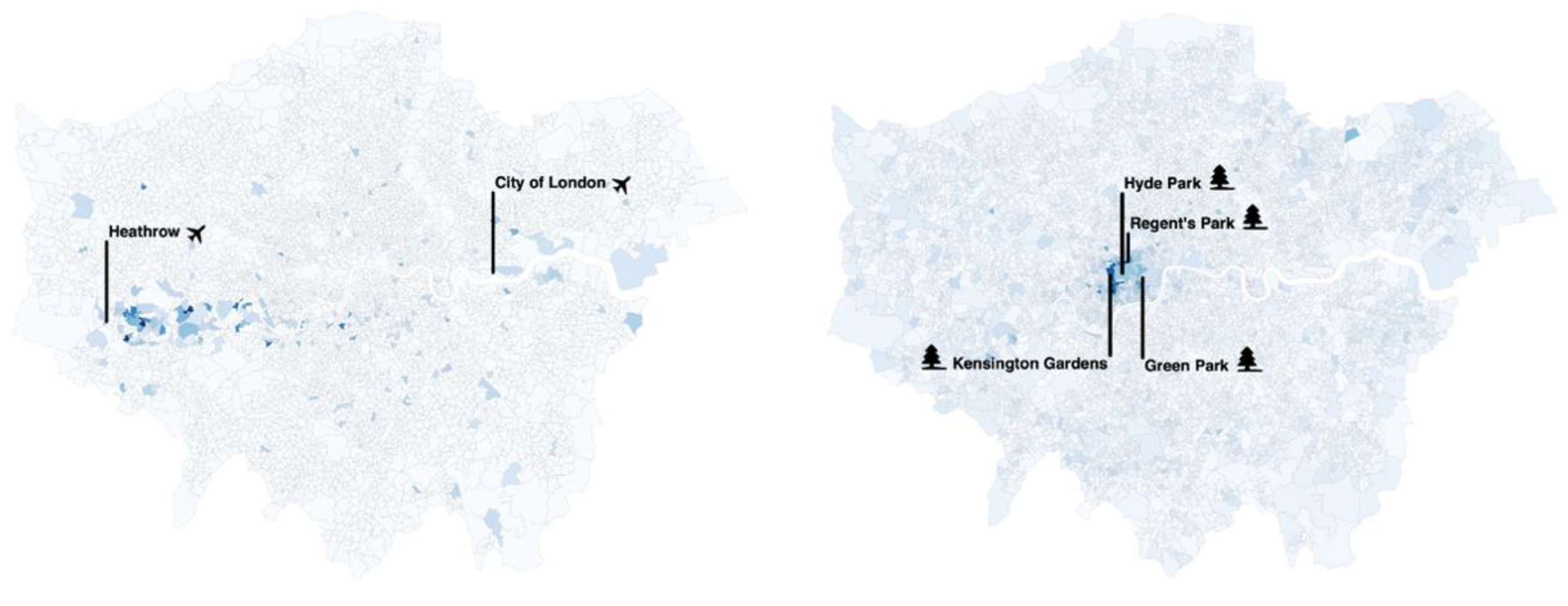
While analyzing all the processed LSOAs in the Greater London atlas, two were found that illustrate the potential of this technique: the Airplane and Potted Plant categories (
Figure A1).
In the case of the first, a higher density of planes was detected per image in the areas next to the airports of Heathrow and the City of London. Moreover, all detected planes were located to the right of each of these structures. This phenomenon is explained by the wind direction being from west to east, which means that the planes land from east to west, and the fact that landing takes significantly longer than taking off. Thus, only images taken on the right contain planes. Finally, the difference in the number of detections next to each of these airports is also clear. Due to the greater volume of air traffic at Heathrow, most of them are in its proximity.
Potted plants were also frequently detected. These were mainly present in images closer to the biggest parks of London. This category includes all vegetation inserted in any type of pot. Given that vegetation was the second most labeled type of pixel across the GSV imagery dataset after executing PSPNet101, the high level of captured potted plants, the fourth most detected object, is not surprising.
Figure A1.
(Left) Density of planes present in images taken next to the closest London airports agrees with expectations. (Right) Identically, the biggest density of potted plants was observed closer to the biggest parks.
Figure A1.
(Left) Density of planes present in images taken next to the closest London airports agrees with expectations. (Right) Identically, the biggest density of potted plants was observed closer to the biggest parks.
Appendix B. YOLOv5 Limitations and Misclassifications
For the objects we defined as relevant to cyclists’ road safety, the number of misclassifications was minimal. This was achieved because a high threshold of 0.5 was defined to count as a detection, and in the MS Coco training dataset, the most common objects are the ones we are interested in.
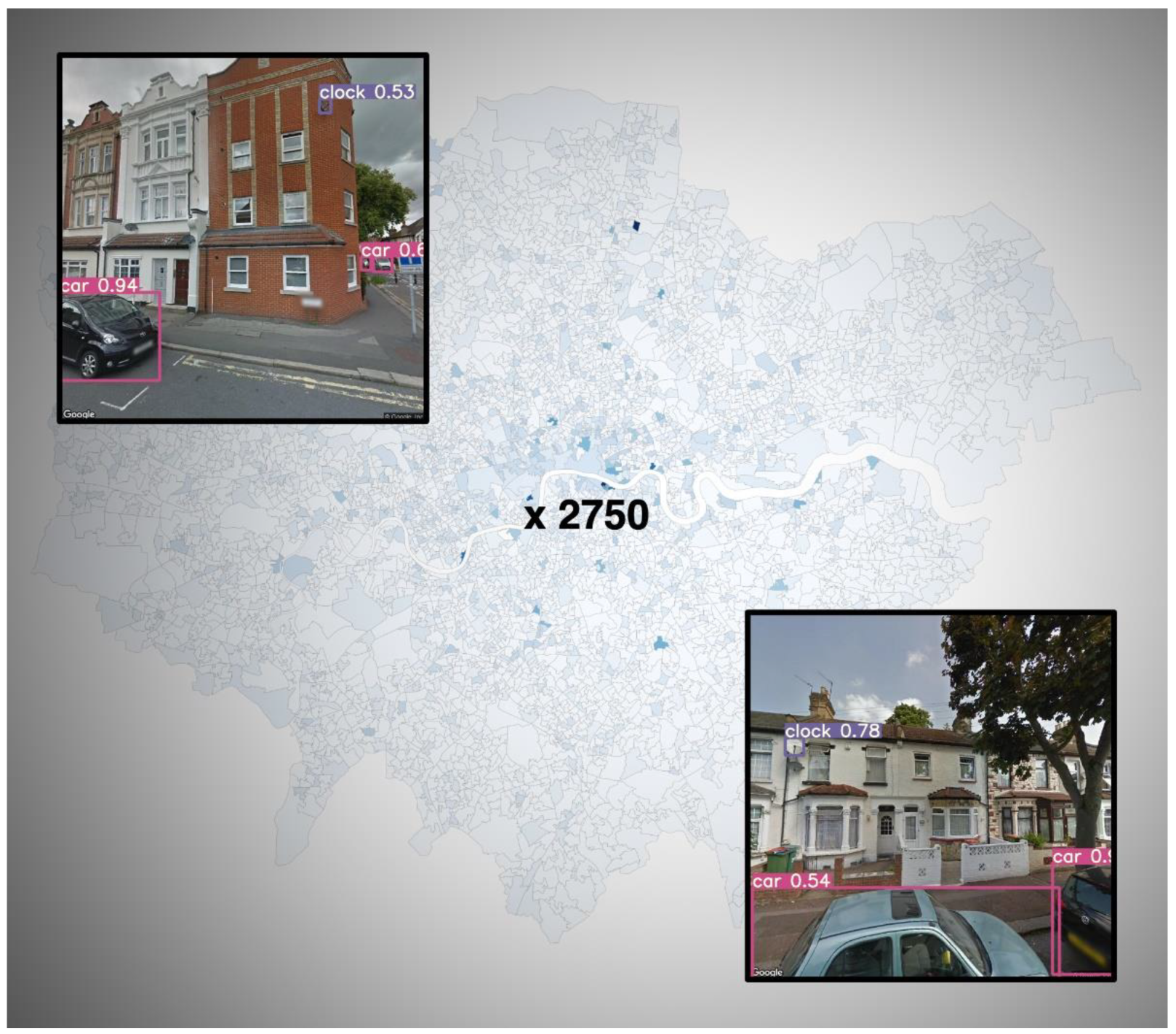
However, there were objects that were consistently misclassified. The most common were satellite dishes being detected as clocks. Depending on the angle, arm dishes can easily resemble a clock pointer. A total of 2750 clocks were detected in the complete GSV imagery dataset (
Figure A2). Other less common objects were also wrongly identified: some due to their shape, others because of their texture. Examples include, for the former, the detection of boats instead of construction containers and, for the latter, benches instead of fences.
Figure A2.
Example of misclassification in YOLOv5.
Figure A2.
Example of misclassification in YOLOv5.
Appendix C. Object Detection Correlation Matrix
Figure A3 presents the correlation matrix for the top 15 detected objects. Thus, each cell contains the Pearson correlation coefficient (top) and the associated
p-value (bottom). Highlighted are the objects car, person, truck, bus and bicycle.
Figure A3.
Correlation matrix of the top 15 detected objects.
Figure A3.
Correlation matrix of the top 15 detected objects.
Appendix D. PSPNet101 and Image Segmentation
Figure A4 illustrates the measurement of road and cycle line widths, these values being important for cyclists’ safety, especially in the context of shared cycling lanes. With a legally enforced distance of over 1.5 m between vehicles and cyclists. A larger width for cycle lanes allows cyclists to maintain a safe distance from other vehicles and navigate around any potential road defects.
Figure A4.
Example illustrating the potential of IS to extract road (left) and sidewalk (right) width.
Figure A4.
Example illustrating the potential of IS to extract road (left) and sidewalk (right) width.
Appendix E. Object Detection and Image Segmentation Examples
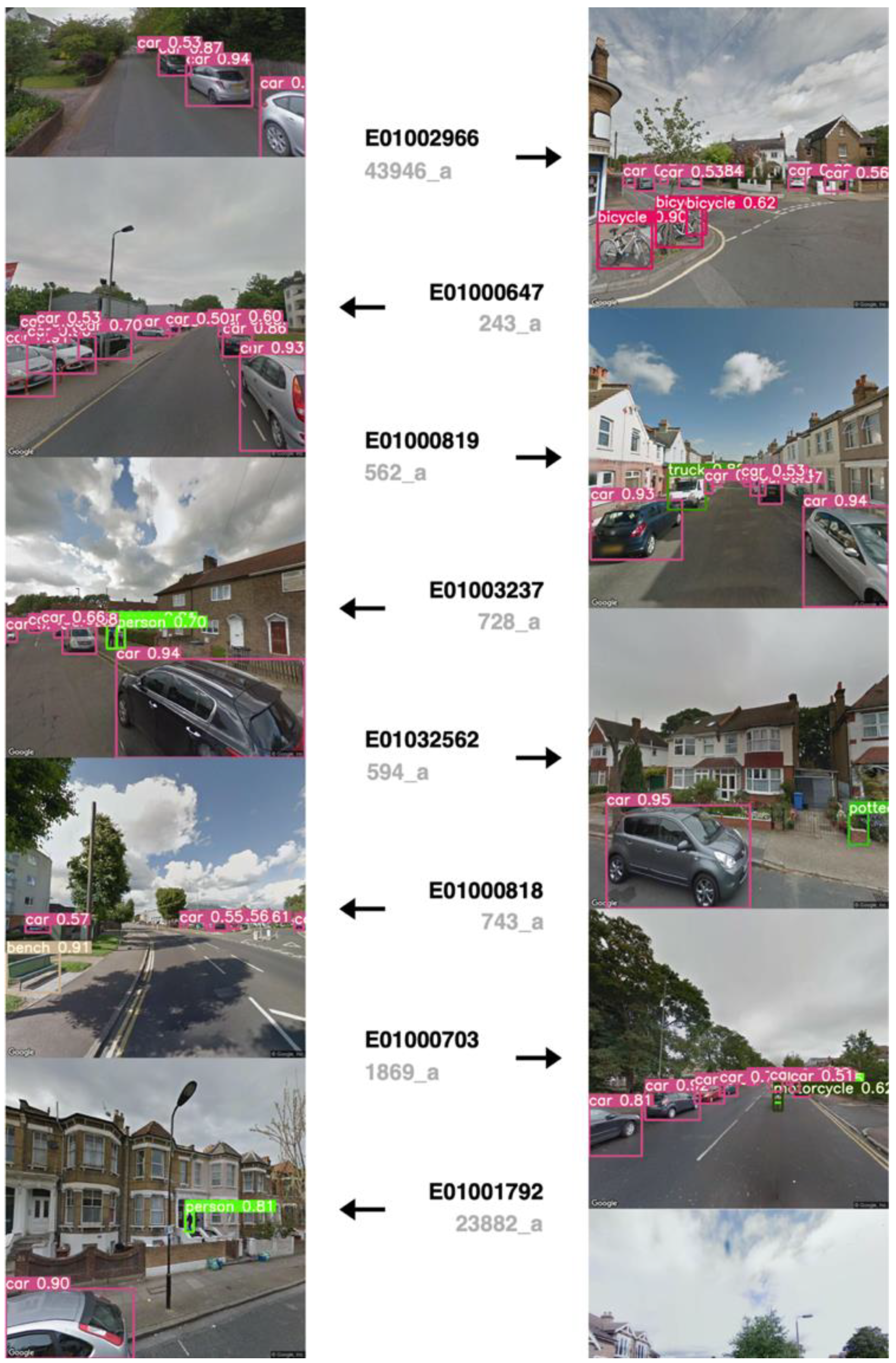
Figure A5 and
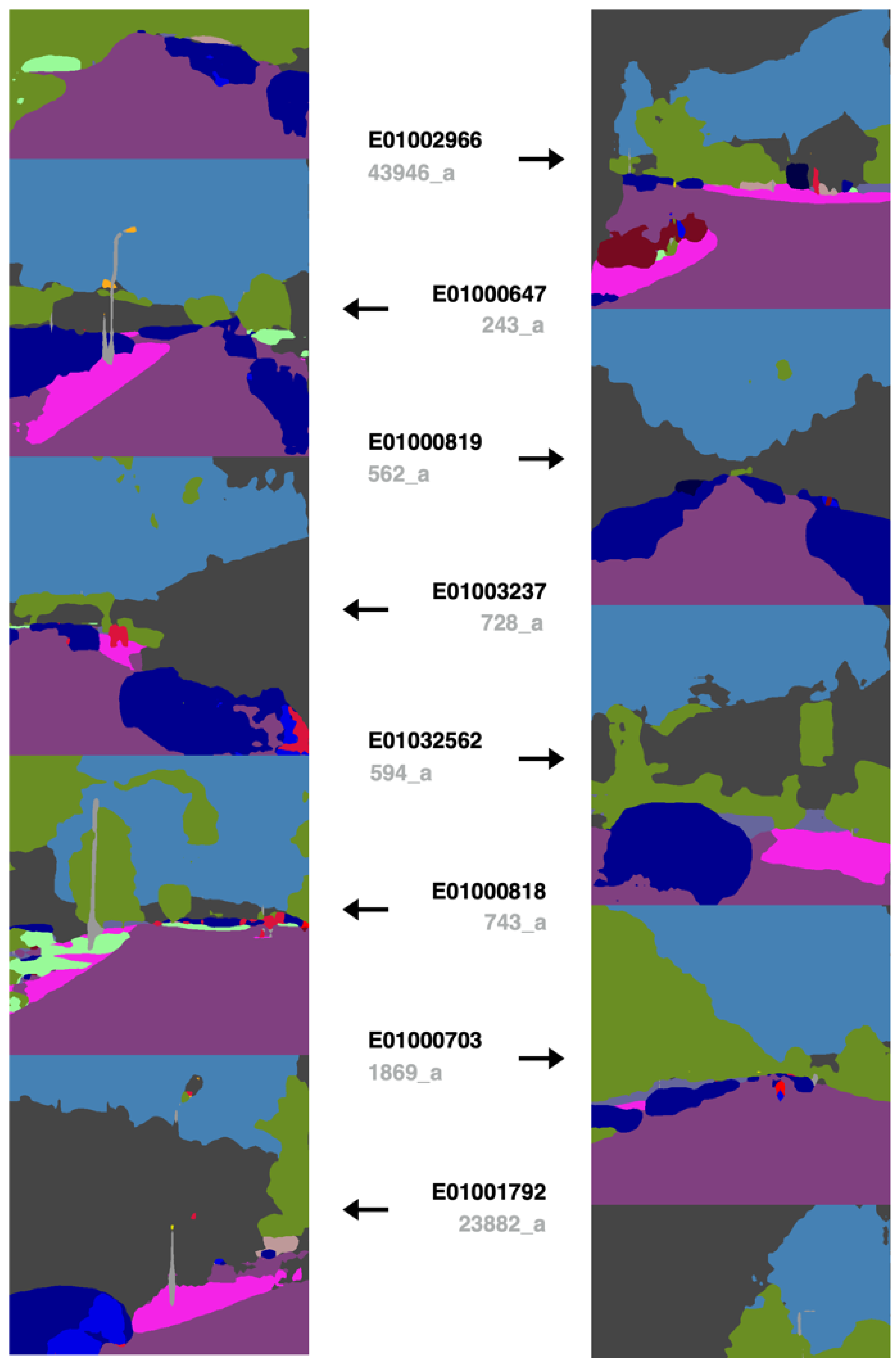
Figure A6 show some random outputs of the approach proposed in this article.
Figure A5.
Ten randomly chosen object detection images from different LSOAs that show high detection accuracy among MS Coco categories.
Figure A5.
Ten randomly chosen object detection images from different LSOAs that show high detection accuracy among MS Coco categories.
Figure A6.
A small sample of randomly segmented images from different LSOAs that show the importance of accounting for structure occlusion while capturing sizes and shapes.
Figure A6.
A small sample of randomly segmented images from different LSOAs that show the importance of accounting for structure occlusion while capturing sizes and shapes.
References
- U.S. Departament of Transportation. “pedbikeinfo”, Pedestrian and Bicycle Information Center. Available online: https://www.pedbikeinfo.org (accessed on 19 April 2020).
- Balogh, S.M. Perceived Safety of Cyclists: The Role of Road Attributes; KTH Royal Institute of Technology: Stockholm, Sweden, 2017. [Google Scholar]
- Centers for Disease Control and Prevention (CDC). Physical Activity: Builds a Healthy and Strong America. Available online: https://www.cdc.gov/physicalactivity/about-physical-activity/pdfs/healthy-strong-america-201902_508.pdf (accessed on 19 April 2020).
- U.S. Environmental Protection Agency. Greenhouse Gas Emissions from a Typical Passenger Vehicle. Available online: https://www.epa.gov/greenvehicles/greenhouse-gas-emissions-typical-passenger-vehicle (accessed on 19 May 2020).
- Gibbs, K.; Slater, S.; Nicholson, N.; Barker, D.; Chaloupka, F. Income Disparities in Street Features that Encourage Walking; A BTG Research Brief; Bridging the Gap Program: Chicago, IL, USA, 2012. [Google Scholar]
- League of American Bicyclists. The New Makority: Pedaling Towards Equity; League of American Bicyclists: Newport, RI, USA, 2013. [Google Scholar]
- Rojas-Rueda, D.; De Nazelle, A.; Tainio, M.; Nieuwenhuijsen, M.J. The health risks and benefits of cycling in urban environments compared with car use: Health impact assessment study. BMJ 2011, 343, d4521. [Google Scholar] [CrossRef]
- de Hartog, J.J.; Boogaard, H.; Nijland, H.; Hoek, G. Do the health benefits of cycling outweigh the risks? Environ. Health Perspect. 2010, 118, 1109–1116. [Google Scholar] [CrossRef] [PubMed]
- Allan, C. UK Cycling Statistics. November 2019. Available online: https://www.cyclinguk.org/statistics (accessed on 19 August 2020).
- Chen, C.; Anderson, J.C.; Wang, H.; Wang, Y.; Vogt, R.; Hernandez, S. How bicycle level of traffic stress correlate with reported cyclist accidents injury severities: A geospatial and mixed logit analysis. Accid. Anal. Prev. 2017, 108, 234–244. [Google Scholar] [CrossRef] [PubMed]
- Janstrup, K.H.; Kaplan, S.; Hels, T.; Lauritsen, J.; Prato, C.G. Understanding traffic crash under-reporting: Linking police and medical records to individual and crash characteristics. Traffic Inj. Prev. 2016, 17, 580–584. [Google Scholar] [CrossRef] [PubMed]
- Veisten, K.; Sælensminde, K.; Alvær, K.; Bjørnskau, T.; Elvik, R.; Schistad, T.; Ytterstad, B. Total costs of bicycle injuries in Norway: Correcting injury figures and indicating data needs. Accid. Anal. Prev. 2007, 39, 1162–1169. [Google Scholar] [CrossRef] [PubMed]
- Debrabant, B.; Halekoh, U.; Bonat, W.H.; Hansen, D.L.; Hjelmborg, J.; Lauritsen, J. Identifying traffic accident black spots with Poisson-Tweedie models. Accid. Anal. Prev. 2018, 111, 147–154. [Google Scholar] [CrossRef]
- SafetyNet. Pedestrians & Cyclists. 2009. Available online: https://ec.europa.eu/transport/road_safety/sites/default/files/specialist/knowledge/pdf/pedestrians.pdf (accessed on 13 May 2020).
- Belin, M.Å.; Johansson, R.; Lindberg, J.; Tingvall, C. The Vision Zero and its consequences. In Proceedings of the 4th International Conference on Safety and Environment in the 21st Century, Tel Aviv, Israel, 23–27 November 1997. [Google Scholar]
- Tingvall, C.; Haworth, N. Vision Zero—An ethical approach to safety and mobility. In Proceedings of the 6th ITE International Conference Road Safety & Traffic Enforcement: Beyond 2000, Melbourne, Australia, 6–7 September 1999. [Google Scholar]
- U.S. Environmental Protection Agency. Sources of Greenhouse Gas Emissions. Available online: https://www.epa.gov/ghgemissions/sources-greenhouse-gas-emissions (accessed on 19 May 2020).
- Hasselwander, M.; Tamagusko, T.; Bigotte, J.F.; Ferreira, A.; Mejia, A.; Ferranti, E.J.S. Building back better: The COVID-19 pandemic and transport policy implications for a developing megacity. Sustain. Cities Soc. 2021, 69, 102864. [Google Scholar] [CrossRef]
- GOV.UK. £2 Billion Package to Create New Era for Cycling and Walking. Available online: https://www.gov.uk/government/news/2-billion-package-to-create-new-era-for-cycling-and-walking (accessed on 19 August 2020).
- Tamagusko, T.; Ferreira, A. Data-Driven Approach to Understand the Mobility Patterns of the Portuguese Population during the COVID-19 Pandemic. Sustainability 2020, 12, 9775. [Google Scholar] [CrossRef]
- Naik, N.; Philipoom, J.; Raskar, R.; Hidalgo, C. Streetscore—Predicting the Perceived Safety of One Million Streetscapes. In Proceedings of the IEEE Conference on Computer Vision and Pattern Recognition Workshops, Columbus, OH, USA, 23–28 June 2014; pp. 793–799. [Google Scholar] [CrossRef]
- Dubey, A.; Naik, N.; Parikh, D.; Raskar, R. Deep Learning the City: Quantifying Urban Perception at a Global Scale. In Proceedings of the Computer Vision–ECCV 2016: 14th European Conference, Amsterdam, The Netherlands, 11–14 October 2016; Volume 3, pp. 196–212. [Google Scholar] [CrossRef]
- Wikipedia. Coverage of Google Street View. Last Modified on 14 August 2020. Available online: https://en.wikipedia.org/wiki/Coverage_of_Google_Street_View (accessed on 19 August 2020).
- Jocher, G. “YOLOv5”, Ultralytics. Available online: https://github.com/ultralytics/yolov5 (accessed on 23 July 2020).
- Zhao, H.; Shi, J.; Qi, X.; Wang, X.; Jia, J. Pyramid scene parsing network. In Proceedings of the IEEE Conference on Computer Vision and Pattern Recognition, Honolulu, HI, USA, 21–26 July 2017; pp. 6230–6239. [Google Scholar] [CrossRef]
- Office for National Statistics Census 2021 Geographies. Guidance about the Different Geographies Used for the Results of Census 2021, for Analysts and Researchers Using Census Data. Available online: https://www.ons.gov.uk/methodology/geography/ukgeographies/censusgeographies/census2021geographies (accessed on 20 April 2020).
- Wiley, V.; Lucas, T. Computer Vision and Image Processing: A Paper Review. Int. J. Artif. Intell. Res. 2018, 2, 22. [Google Scholar] [CrossRef]
- Lecun, Y.; Bengio, Y.; Hinton, G. Deep learning. Nature 2015, 521, 436–444. [Google Scholar] [CrossRef]
- Dinov, I.D. Data Science and Predictive Analytics: Biomedical and Health Applications Using R, 1st ed.; Springer International Publishing Imprint: Springer: Cham, Switzerland, 2018; ISBN 978-3-319-72347-1. [Google Scholar]
- Mishra, R.K.; Reddy, G.Y.S.; Pathak, H. The Understanding of Deep Learning: A Comprehensive Review. Math. Probl. Eng. 2021, 2021, 5548884. [Google Scholar] [CrossRef]
- European Commission. European Road Safety Charter. Available online: https://webgate.ec.europa.eu/multisite/ersc/node_en (accessed on 19 May 2020).
- Useche, S.A.; Montoro, L.; Sanmartin, J.; Alonso, F. Healthy but risky: A descriptive study on cyclists’ encouraging and discouraging factors for using bicycles, habits and safety outcomes. Transp. Res. Part F Traffic Psychol. Behav. 2019, 62, 587–598. [Google Scholar] [CrossRef]
- Sanders, R.L. Perceived traffic risk for cyclists: The impact of near miss and collision experiences. Accid. Anal. Prev. 2015, 75, 26–34. [Google Scholar] [CrossRef] [PubMed]
- Branion-Calles, M.; Götschi, T.; Nelson, T.; Anaya-Boig, E.; Avila-Palencia, I.; Castro, A.; Cole-Hunter, T.; de Nazelle, A.; Dons, E.; Gaupp-Berghausen, M.; et al. Cyclist crash rates and risk factors in a prospective cohort in seven European cities. Accid. Anal. Prev. 2020, 141, 105540. [Google Scholar] [CrossRef] [PubMed]
- Aldred, R.; Crosweller, S. Investigating the rates and impacts of near misses and related incidents among UK cyclists. J. Transp. Health 2015, 2, 379–393. [Google Scholar] [CrossRef]
- Lawson, A.R.; Ghosh, B.; Pakrashi, V. Quantifying the perceived safety of cyclists in Dublin. Proc. Inst. Civ. Eng. Transp. 2015, 168, 290–299. [Google Scholar] [CrossRef]
- Mobiel 21; Bike Citizens. PING if you care!—Crowdsourcing the Urban Cycling Experience. Available online: https://pingifyoucare.eu/ (accessed on 11 January 2022).
- Transport for London (TfL). Travel in London, Report 11. Available online: http://content.tfl.gov.uk/travel-in-london-report-11.pdf (accessed on 19 April 2020).
- Teschke, K.; Harris, M.A.; Reynolds, C.C.O.; Winters, M.; Babul, S.; Chipman, M. Route Infrastructure and the Risk of Injuries to Bicyclists: A Case-Crossover Study. Am. J. Public Health 2012, 102, 2336–2343. [Google Scholar] [CrossRef]
- Johnson, M.; Newstead, S.; Oxley, J.; Charlton, J. Cyclists and open vehicle doors: Crash characteristics and risk factors. Saf. Sci. 2013, 59, 135–140. [Google Scholar] [CrossRef]
- Chen, L.; Chen, C.; Srinivasan, R.; Mcknight, C.E.; Ewing, R.; Roe, M. Evaluating the Safety Effects of Bicycle Lanes in New York City. Am. J. Public Health 2012, 102, 300319. [Google Scholar] [CrossRef]
- Department of Health. State Government of Victoria. Cycling—Preventing Injury. Available online: https://www.betterhealth.vic.gov.au/health/HealthyLiving/cycling-preventing-injury (accessed on 7 May 2020).
- World Health Organization. Road Safety—Speed. Available online: https://www.who.int/violence_injury_prevention/publications/road_traffic/world_report/speed_en.pdf (accessed on 19 April 2020).
- European Commission. Speed and Accident Risk. Available online: https://ec.europa.eu/transport/road_safety/specialist/knowledge/speed/speed_is_a_central_issue_in_road_safety/speed_and_accident_risk_en (accessed on 8 May 2020).
- European Commission. What Forces Can Be Tolerated the Human Body? Available online: https://ec.europa.eu/transport/road_safety/specialist/knowledge/vehicle/key_issues_for_vehicle_safety_design/what_forces_can_be_tolerated_the_human_body_en (accessed on 9 May 2020).
- Pasanen, E. Driving Speeds and Pedestrian Safety (Written in Finnish); Helsinki University: Helsinki, Finland, 1991. [Google Scholar]
- International Road Assessment Programme (iRAP). Bicycle Facilities, Road Safety Toolkit. Available online: http://toolkit.irap.org/default.asp?page=treatment&id=1 (accessed on 8 April 2020).
- Road Safety Commission. Government of Western Australia. The Safety of People Walking and Riding Cyclists. Available online: https://www.rsc.wa.gov.au/RSC/media/Documents/Resources/Cyclists-INFO-SHEET.pdf (accessed on 8 April 2020).
- U.S. Departament of Transportation. National Highway Traffic Safety Administration. Bicycle Safety. Available online: https://www.nhtsa.gov/road-safety/bicycle-safety (accessed on 8 April 2020).
- Asgarzadeh, M.; Verma, S.; Mekary, R.A.; Courtney, T.K.; Christiani, D.C. The role of intersection and street design on severity of bicycle-motor vehicle crashes. Inj. Prev. 2017, 23, 179–185. [Google Scholar] [CrossRef]
- Dablanc, L. Goods transport in large European cities: Difficult to organize, difficult to modernize. Transp. Res. Part A Policy Pract. 2007, 41, 280–285. [Google Scholar] [CrossRef]
- Jaller, M.; Holguín-veras, J.; Hodge, S.D. Parking in the City Challenges for Freight Traffic. J. Transp. Res. Board 2013, 2379, 46–56. [Google Scholar] [CrossRef]
- Conway, A.; Tavernier, N.; Leal-tavares, V.; Gharamani, N.; Chauvet, L.; Chiu, M.; Yeap, X.B. Freight in a Bicycle-Friendly City Exploratory Analysis with New York City Open Data. J. Transp. Res. Board 2016, 2547, 91–101. [Google Scholar] [CrossRef]
- Kim, J.; Kim, S.; Ulfarsson, G.F.; Porrello, L.A. Bicyclist injury severities in bicycle—Motor vehicle accidents. Accid. Anal. Prev. 2007, 39, 238–251. [Google Scholar] [CrossRef]
- Manson, J.; Cooper, S.; West, A.; Foster, E.; Cole, E.; Tai, N.R.M. Major trauma and urban cyclists: Physiological status and injury profile. Emerg. Med. J. 2012, 30, 32–37. [Google Scholar] [CrossRef] [PubMed]
- Kaplan, S.; Vavatsoulas, K.; Prato, C.G. Aggravating and mitigating factors associated with cyclist injury severity in Denmark. J. Safety Res. 2014, 50, 75–82. [Google Scholar] [CrossRef]
- Chen, P.; Shen, Q. Built environment effects on cyclist injury severity in automobile-involved bicycle crashes. Accid. Anal. Prev. 2016, 86, 239–246. [Google Scholar] [CrossRef]
- Pokorny, P.; Drescher, J.; Pitera, K.; Jonsson, T. ScienceDirect ScienceDirect ScienceDirect Accidents Accidents between between freight freight vehicles vehicles and and bicycles, with a a focus focus on on urban urban areas areas. Transp. Res. Procedia 2017, 25, 999–1007. [Google Scholar] [CrossRef]
- McCarthy, M.; Gilbert, K. Cyclist road deaths in London 1985–1992: Drivers, vehicles, manoeuvres and injuries. Accid. Anal. Prev. 1996, 28, 275–279. [Google Scholar] [CrossRef]
- Morgan, A.S.; Dale, H.B.; Lee, W.E.; Edwards, P.J. Deaths of cyclists in London: Trends from 1992 to 2006. BMC Public Health 2010, 10, 699. [Google Scholar] [CrossRef]
- Departament for Transport. Traffic Advisory Leaflet 5/96. Available online: https://webarchive.nationalarchives.gov.uk/ukgwa/20090505152230/http://www.dft.gov.uk/adobepdf/165240/244921/244924/TAL_5-96 (accessed on 23 May 2023).
- Tuckel, P.; Milczarski, W.; Maisel, R. Pedestrian injuries due to collisions with bicycles in New York and California. J. Safety Res. 2014, 51, 7–13. [Google Scholar] [CrossRef] [PubMed]
- European Commission. Intelligent Energy Europe. Promoting Cycling for Everyone as a Daily Transport Mode (PRESTO). Available online: https://ec.europa.eu/energy/intelligent/projects/sites/iee-projects/files/projects/documents/presto_fact_sheet_cyclists_and_pedestrians_en.pdf (accessed on 11 May 2020).
- Wikipedia. Object detection. Last modified on 24 July 2020. Available online: https://en.wikipedia.org/wiki/Object_detection (accessed on 19 August 2020).
- Wikipedia. Image Segmentation. Last modified on 6 July 2020. Available online: https://en.wikipedia.org/wiki/Image_segmentation (accessed on 19 August 2020).
- Papers with Code. Semantic Segmentation on Cityscapes Test. State-of-the-Art. Available online: https://paperswithcode.com/sota/semantic-segmentation-on-cityscapes (accessed on 18 August 2020).
- Lin, T.; Maire, M.; Belongie, S.; Hays, J.; Perona, P.; Ramanan, D.; Doll, P. Microsoft COCO: Common Objects in Context. In Proceedings of the Computer Vision–ECCV 2014: 13th European Conference, Zurich, Switzerland, 6–12 September 2014; pp. 740–755. [Google Scholar]
- Kuznetsova, A.; Rom, H.; Alldrin, N.; Uijlings, J.; Krasin, I.; Kamali, S.; Popov, S.; Malloci, M.; Kolesnikov, A.; Duerig, T.; et al. The Open Images Dataset V4 Unified Image Classification, Object Detection, and Visual Relationship Detection at Scale. Int. J. Comput. Vis. 2020, 128, 1956–1981. [Google Scholar] [CrossRef]
- Cordts, M.; Ramos, S.; Rehfeld, T.; Enzweiler, M.; Roth, S.; Daimler, A.G.R.D.; Darmstadt, T.U.; Informatics, M.P.I.; Dresden, T.U. The Cityscapes Dataset for Semantic Urban Scene Understanding. In Proceedings of the IEEE conference on computer vision and pattern recognition, Caesars Palace, 27–30 June 2016; pp. 3213–3223. [Google Scholar] [CrossRef]
- Zhou, B.; Zhao, H.; Puig, X.; Fidler, S.; Barriuso, A.; Torralba, A. Scene Parsing through ADE20K Dataset. In Proceedings of the IEEE Conference on Computer Vision and Pattern Recognition, Honolulu, HI, USA, 21–26 July 2017; pp. 5122–5130. [Google Scholar] [CrossRef]
- Greater London Authority Lower Super Output Area in Greater London Atlas. Available online: https://data.london.gov.uk/dataset/lsoa-atlas (accessed on 18 May 2020).
| Disclaimer/Publisher’s Note: The statements, opinions and data contained in all publications are solely those of the individual author(s) and contributor(s) and not of MDPI and/or the editor(s). MDPI and/or the editor(s) disclaim responsibility for any injury to people or property resulting from any ideas, methods, instructions or products referred to in the content. |
© 2023 by the authors. Licensee MDPI, Basel, Switzerland. This article is an open access article distributed under the terms and conditions of the Creative Commons Attribution (CC BY) license (https://creativecommons.org/licenses/by/4.0/).
