Intelligent Identification and Prediction Mineral Resources Deposit Based on Deep Learning

Abstract

In recent years, the intelligent identification and prediction of ore deposits based on deep learning algorithm and image processing technology has gradually become one of the main research frontiers in the field of geological and metallogenic prediction. However, this method also has many problems that need to be solved. For example: (1) There are very few trainable image samples containing mineral point labels; (2) the geological image features are small and irregular, and the image similarity is high; (3) it is difficult to calculate the influence of different geological prospecting factors on ore mineralization. Based on this, this paper constructs a deep learning network model multiscale feature attention framework (MFAF) based on geoimage data. The results show that the MFCA-Net module in the MFAF model can solve the problem of scarce mine label images to a certain extent. In addition, the channel attention mechanism SE-Net module can quantify the difference in influence of different source factors on mineralization. The prediction map is obtained by applying the MFAF model in the study of deposit identification and prediction in the research area of the southern section of the Qin-hang metallogenic belt. The experimental results show that the areas numbered 5, 9, 16, 28, 34, 41, 50, 72, 74, 75, 80, 97, 101, 124, and 130 have great metallogenic potential and this method would be a promising tool for metallogenic prediction. A large number of experimental results show that this method has obvious advantages over other state-of-the-art methods in the prediction of prospecting target areas, and the prediction effect in the samples with mines is greatly improved. The multi-scale feature fusion and attention mechanism MFAF in this paper can provide a new way of thinking for geologists in mineral exploration. The research of this paper also provides resource guarantees and technical support for the sustainable exploitation of mineral resources and the sustainable growth of society and economy.

1. Introduction

Mineral resources are an important resource guarantee for sustainable economic growth and stable social development. With the continuous exploitation and consumption of mineral deposits, many precious resources are facing the risk of scarcity. Therefore, geologists began to explore new techniques and methods to find new deposits. In recent years, most of the geological prospecting research uses single data source analysis, such as geological mapping technology, geochemical metallogenic prediction, geophysical metallogenic prediction, or remote sensing image prediction. A few scholars use artificial intelligence image processing techniques to predict mineral deposits. With the development of artificial intelligence and big data technology in geology, intelligent prediction of mineral resources based on machine learning algorithm and image processing technology has gradually become one of the frontier hot spots for geologists and scientific researchers [1,2,3]. Many scholars use logistic regression [4], support vector machine (SVM) [5], genetic algorithm [6], random forest (RF) [7], artificial neural network (ANN) [8], and other artificial intelligence algorithms to carry out intelligent prediction and mineral analysis of geological and mineral resources. It is proven that machine learning and deep learning algorithms have a strong prediction ability in identifying the nonlinear relationship between ore deposits and metallogenic conditions and can significantly improve the accuracy and success rate of prediction.

However, deep learning technology is still in its exploratory stage in mining and forecasting geological prospecting information, and there are still some problems to be solved. Common problems include: (1) Due to the scarcity of mineral points in the study area, trainable image samples containing mineral point labels are very few; (2) due to the fine and irregular features of geological images, the image similarity is substantial and it is difficult to extract effective information; (3) the variation in the degree of influence of geological prospecting factors of different data sources on ore mineralization. All these problems bring more challenges and opportunities for geological workers in ore deposit prediction. Through our research on previous journals, no one has yet adopted deep learning combined with attention mechanisms to analyze the main ore-forming factors and ore-forming prediction areas of ore deposits. The research questions and objectives are: (1) How to enhance the labeled geological image samples? (2) how to use the attention mechanism to assign different weight coefficients to different geological image data and avoid the influence of human factors? (3) which artificial intelligence model can be used to identify and predict ore deposits in the research area more effectively? Based on the above research questions and objectives, in this paper, the Jinshan research area in the southern section of the Qin-hang metallogenic belt of China is taken as the study area. A deep learning model of multiscale feature attention framework (MFAF) is proposed to construct a forecast map of deposit identification and prediction based on sediment geochemical data and a mineral geological map. This method may improve the accuracy and success rate of metallogenic prediction with different data sources and both fine and irregular features of geological images.

2. Literature Review

2.1. Deep Learning for Metallogenic Prediction

Deep learning has been actively applied in geological information metallogenic prediction and has achieved many innovative results [9,10,11,12,13,14]. Zuo and Carranza [15] used the SVM algorithm to predict the Nova Scotia gold deposit in western Canada, which confirmed that the SVM algorithm has obvious advantages in prediction accuracy and precision compared with the traditional weight of evidence method. Daviran et al. [16] used a genetic algorithm to optimize the super parameters of random forest (RF) to improve the accuracy of mine target prediction. Chen et al. [17] proposed a novel ensemble scheme for MPM using a wavelet neural network (WNN) and Monte Carlo simulations (MCs) to address the forementioned issues. The resulting predictive map provides important clues for W-Sn deposit occurrences, which could stimulate future mineral exploration in the Nanling Range. Marjanovic et al. [18] adopted convolutional neural network (CNN), recurrent neural network (RNN), and multilayer perceptron (MLP) and RF machine learning algorithms to analyze mineral composition data from 488 sediment samples. The results show that trained machine learning models can help experts analyze mineral composition more efficiently and reliably.

In previous studies, some scholars have used CNN methods [19], deep convolutional neural network (DCNN) [20] and long short-term memory network (LSTMN) [21], generative adversarial network (GAN) [22], transfer learning (TL) [23], and other deep learning algorithms to carry out intelligent prediction of geochemical mineral resources, proving that deep learning algorithms are a powerful tool for geochemical element concentration analysis and metallogenic prediction. For example, Chen and Shayilan [24] used deep learning technology to establish a learning model for multi-geochemical anomaly detection oriented to prospecting targets. The test results show that the model algorithm is worthy of further study in the field of prospecting with complex geochemical backgrounds. He et al. [25] made a review of the research of machine learning in the field of geochemistry, and the research results predicted that deep learning and machine learning technology would achieve great breakthroughs in the research of geochemistry. Huang et al. [26] used the deep learning method to capture the characteristics of geochemical elements and build a deep intelligent prospecting target prediction framework. The experimental results show that the multi-scale feature deep learning framework has significant advantages compared with other deep learning methods.

2.2. Multi-Scale Feature Fusion Technology for Mineral Prospecting

In recent years, some geological experts have applied multi-scale feature fusion technology to geological prospecting and geochemical analysis and achieved fruitful results. For example, Guan et al. [27] proposes a feature fusion convolutional autoencoder to extract and fuse the spatial structural features and compositional relationships of multivariate geochemicals for identifying geochemical anomalies. The results show that the method is applicable and reliable for mineral resource exploration. Zhou et al. [28] combined multi-scale geophysical prospecting technology with geological prospecting in typical deposit areas to provide evidence for geologists to understand the metallogenic background and discover new deposits. Li et al. [29] presents a multi-modal feature fusion based framework to improve the geographic image annotation. The comprehensive experiments show that this feature fusion based method achieves much better performances compared to traditional methods.

2.3. The Mechanism of Attention Used in Geodata Analysis

At present, many scholars have conducted in-depth studies on the mechanism of attention and achieved good results [30,31,32]. Some earth science experts have combined the channel attention mechanism with geoscience images, and the image classification effect has been significantly improved. For example, Zhu et al. [33] proposed super-resolution model employs residual channel attention networks as a backbone structure. The experimental results confirmed that the enhanced multi-temporal images can bring substantial improvements to classification. Gajbhiye et al. [34] combined the channel attention mechanism and convolutional neural network to generate letters for remote sensing images and conducted model evaluation in the test set, obtaining good results. Additionally, many scholars have integrated the spatial attention module into the deep learning network model to improve the training effect of the model [35,36,37]. Some geological experts focus on the spatial distribution of geological images and data and achieve good results in image modeling and image classification. For example, Pan et al. [38] proposed an integrated method to effectively integrate multi-source complex spatial data, which combined a spatial model with complex stratigraphic modeling technology to realize the visualization of the spatial model. Zhao and Wang [39] used the machine learning method to analyze the spatial distribution of geochemical elements such As Au, As, Sb, and Hg. The results show that the geochemical anomalies extracted using this method are consistent with the known metallogenic areas, which proves that this method is feasible and effective in identifying geochemical anomalies.

3. Materials and Methods

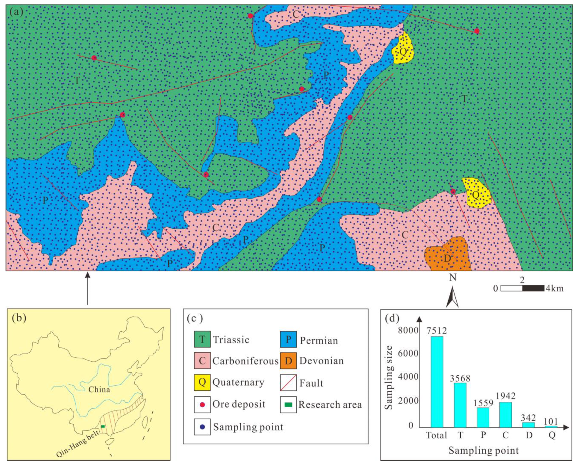
3.1. Materials

The study area Jinshan is located in the southern section of China’s Qin-hang (Qinzhou Bay—Hangzhou Bay) metallogenic belt, which is a giant structural junction belt located in the middle of two ancient landmasses (Yangtze and Huaysia). The belt extends from Hangzhou Bay in the northeast to Qinzhou Bay in the southwest with a total length of 2000 km and has good metallogenic potential. Figure 1 shows a general map of geology and mineral resources in the study area. Red dots are known deposit locations and blue dots are stream sediment sampling locations. There are five major strata in the study area: Triassic, Permian, Carboniferous, Devonian, and Quaternary. Among them, the Triassic lithologic is given priority to gray, gray, sandy mudstone, lower than the white, thin layer and, therefore, tuffaceous shale. Permian lithology is light gray thick-bedded bioclastic limestone, sand-clastic limestone, and microcrystalline limestone. The Carboniferous lithology is composed of gray middle-thick bedded bioclastic limestone, gray-white thick bedded dolomite, and biooritic microcrystalline limestone. Devonian lithology is dark gray thin bedded limestone, microcrystalline limestone, and marbled limestone. The structural development in this area is dominated by faults, including regional major faults, northeast trending faults, northwest faults, near south–north faults, and interlayer fracture zones. Regional metallogenic composition is influenced by lithology and tectonic common control and the Triassic ore formation. Therefore, known ore deposits are situated near the faults and fissures, obviously controlled by fracture structure. The data sources analyzed in this study include mineral geological maps and stream sediment geochemical element data. According to statistics, we sampled 3568, 1559, 1942, 342, and 101 samples from each formation, for a total of 7512 samples. The data analyzed via stream sediment survey include Ag, Au, B, Sn, Cu, Ba, Mn, Pb, Zn, As, Sb, Hg, Mo, W, Bi, and F.

Table 1. Geochemical element data set (The units of Au and Ag are ng/g, other element units are μg/g).

X	Y	Ag	Au	B	Sn	Cu	Ba	Mn	Pb	Zn	As	Sb	Hg	Mo	W	Bi	F
421.63	2416.85	0.078	0.54	4	2.56	7	88	209	12	23	0.9	0.29	0.04	0.82	1.16	0.42	204
420.93	2416.80	0.06	0.81	3	3.74	5	885	305	33	22	0.58	0.36	0.04	0.82	1.11	1.41	222
420.95	2416.35	0.086	0.94	4	2.41	5	797	267	53	35	1.15	0.34	0.09	0.51	1.16	0.42	212
421.21	2415.85	0.043	0.81	3	1.52	5	1111	423	42	14	0.51	0.35	0.07	0.59	0.38	0.23	222
420.30	2416.35	0.046	0.37	2	1.65	6	941	498	38	17	0.53	0.31	0.02	0.57	0.33	0.61	222
419.86	2416.15	0.033	1.09	4	1.53	8	427	338	37	29	0.74	0.28	0.07	1.68	0.73	0.47	204

shows that part of the geochemical element data, X and Y, correspond to sampling point coordinates.

3.2. Methods

3.2.1. Data Pre-Processing

In this study, the preprocessing of the original geological data is divided into four steps.

(1) Screen out favorable geochemical elements for mineralization. In this study, the support vector model was used to obtain the area under curve (AUC) value of each element, and the Z_AUC value was calculated using Formulas (1)–(3):

$$Q_1=\frac{AUC}{2-AUC}, Q_2=\frac{2AU{C}^2}{1+AUC}$$

(1)

$$S_{AUC}=\sqrt{\frac{AUC\left(1-AUC\right)+\left(C_p-1\right)\left(Q_1-AU{C}^2\right)+\left(C_n-1\right)\left(Q_2-AU{C}^2\right)}{C_p\times C_n}}$$

(2)

$$Z_{AUC}=\frac{AUC-0.5}{S_{AUC}}$$

(3)

The random variable Z_AUC meets the standard normal distribution, and the critical value is obtained by comparing the standard normal distribution table, which is used to detect whether there is a significant difference between AUC and 0.5. The results are shown in

Table 2. The results of AUC and Z_AUC.

Element	AUC	ZAUC	Element	AUC	ZAUC
Au	0.6024	2.8395	B	0.5901	2.4839
Sn	0.6065	2.9595	Cu	0.6311	3.6977
Ag	0.6762	5.1563	Ba	0.6147	3.2020
Mn	0.5573	1.5617	Pb	0.5778	2.1341
Zn	0.5450	1.2232	As	0.5655	1.7893
Sb	0.5942	2.6017	Bi	0.5901	2.4839
Hg	0.6393	3.9516	Mo	0.5983	2.7203
W	0.5778	2.1341	F	0.5696	1.9037

. When the Z_AUC value is greater than 0.01, the critical value of 2.58 is selected; that is, Ag, Au, Sn, Cu, Ba, Sb, Hg, and Mo are selected as favorable prospecting factors.

(2) The inverse distance weight method was used to interpolate the above eight geochemical element data sets, and the corresponding element concentration contour map was obtained. This interpolation calculation experiment references [40] and the experimental results generated T grid points of element concentration map, where W is the width of the image, H is the height, and T is the number of element distribution maps. The calculation formula of the inverse distance weighting method is shown in (4) and (5), where the Euclidean distance from the discrete point (x_i, y_i) to the grid point (x₀, y₀) is the valuation of the position, i is the observed value at the discrete point, and N is the number of discrete points involved in the calculation. In this study, the inverse distance weight method was applied to Ag, Au, Sn, Cu, Ba, Sb, Hg, Mo, and other elements to generate eight isoline maps of element concentration with a size of 1560 × 1560. Finally, the isoline map of element concentration, the geological layer, and the fault structure layer were superimposed with the known ore deposit layer, respectively, to generate 10 new images of geological prospecting factors, as shown in Figure 2.

$$D_i=\sqrt{{(x_0-x_i)}^2+{(y_0-y_i)}^2}$$

(4)

$$Z\left(x_0,y_0\right)={\displaystyle \sum }_{i=1}^N\frac{1}{{(D_i)}^2}{Z}_i/{\displaystyle \sum }_{i=1}^N\frac{1}{{(D_i)}^2}$$

(5)

(3) This step further processes the geoimage generated in Step 2 to obtain the geoimage data set. Firstly, a sliding window is defined, and the element content of each sampling point is obtained by sliding the geographic image with the appropriate step size. After many experiments, the geographic image data set required by the cost research is generated. It is assumed that the geoinformation training set contains N samples, which are various characteristic elements and are their corresponding real labels. C is the number of geological information channels, where 0 represents “no ore” data and 1 represents “ore” data. In this experiment, 128 × 128 windows and 128 pixels were used for sliding operation on the geoinformation map to generate the geoimage data set needed for the final model training. This image data set includes 428 image data (128 × 128 × 10), among which 342 data are included in the training set, including 56 “ore” data and 286 “no ore” data. The test set contains 86 data, including 14 “ore” data and 72 “no ore” data.

(4) Enhance the number of geological images generated in the previous step with Smote. In order to effectively train the deep learning network model, this experiment enhanced the image data by adding Gaussian noise with an average value of 0 and a variance of 0.01. In this paper, according to smote algorithm [41] and the SMOTE method [42], we gave a sample extension to the original geoscience image data set, and enhanced the completeness of the deep learning training model. Through this step, the final generated data set includes 654 data (128 × 128 × 10), among which 524 data are generated in the training set, including 224 “ore” data and 300 “no ore” data. The test set has 130 data, including 56 “ore” data and 74 “no ore” data. After data preprocessing in these four steps, the geoimage data set generated can be used as the input data of the MFAF in this study.

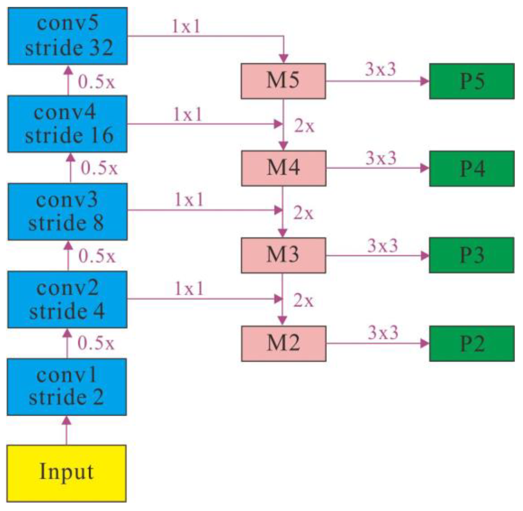
3.2.2. Multiscale Feature Attention Framework (MFAF)

The framework of MFAF research is shown in Figure 3. It mainly consists of two parts: multiscale feature channel attention net (MFCA-Net) and convolution spatial attention net (CSA-Net). MFCA-Net uses the set of expansion coefficients α = {α1, α2, α3, …, αn} and the channel attention mechanism squeeze and excitation block (SE-Net) module. The framework consists of three steps: (1) The expansion coefficient set α is used to generate convolution kernels of different scales, and the feature maps of different scales are obtained to solve the question of a small number of known deposits in the study area and to provide data support for the convolution operation to extract more and more detailed feature information in this area. (2) The feature image generated after expansion convolution will pass through the channel attention module, which comprises both compression and excitation processes. In the compression stage, the global compression feature quantity is obtained via global pooling on the feature graph. At the bottleneck phase, the weights of each channel in the feature map are obtained through a bottleneck structure that is fully connected at two layers, and the weighted feature map is used as input to the next layer network. Therefore, the extracted features are re-calibrated, and different weight values are assigned to the features in different channels $\mathrm{W}=\left\{{\mathrm{W}}_1,{\mathrm{W}}_2,\dots ,{\mathrm{W}}_{\mathrm{n}}\right\}$, so as to solve the problem that different geochemical elements have different influence degrees on mineralization. (3) The CSA-Net module mainly includes a series of convolution operations. Considering that the element contents of different spatial locations in the feature map have different influences on mineralization, the last layer of convolution is added with the spatial attention module to assign different weight coefficients to the features of different locations. In order to reduce the number of training parameters and accelerate the model convergence, each channel was finally classified by the shared full connection layer.

3.2.3. Multi-Scale Feature Fusion

With the deepening of the number of layers in the deep learning network, the semantic expression ability is enhanced; however, this also reduces the resolution of the image, and many detailed features become more and more fuzzy after the convolution operation of the multi-layer network. The traditional target detection model results in the reduction of the effective information of small targets on the last feature map. In this paper, multi-scale feature fusion is used to solve this problem. Instead of using the feature map of the last layer for detection, multi-layer features are selected for fusion and then detection so as to obtain images of multiple scales, and then the classification algorithm is adopted to realize the task of image classification [43,44]. The multi-scale feature fusion diagram is shown in Figure 4.

In order to solve the problem of few mineral points and few ore-bearing label images in the study area, geological layers, fracture images, and a variety of geochemical elements can be used to generate geological image data of different scales, and image data sets can be generated by asynchronously long sliding windows to increase the diversity of data samples. For the input geological data bases set $x^{\prime }={\left\{x_i\right\}}_{i=1}^N$, the expansion coefficient set α = {α₁, α₂, α₃, …, α_n} generates convolution of different sizes to check the convolution operation and generates an image of multi-scale features. Specifically, we use the convolution operation of the convolution kernel $M=\{M_1,M_2,\dots ,M_n\}$ and the set α of expansion coefficients to obtain the multi-scale feature graph F = {F₁, F₂, …, F_n}, where the ith feature is $F_i$. The specific generation Formula (6) is shown as follows: Where x_i represents the ith feature element, M_i represents the convolution weight corresponding to the generation of the ith feature graph, α_i represents the expansion convolution coefficient corresponding to the generation of the ith feature graph, and r represents the convolution channel.

$$F_i=r\left(x_i,M_i,{\alpha }_i\right)$$

(6)

3.2.4. Channel Attention

In the research of deep learning algorithms, the channel attention (CA) mechanism is a resource allocation mechanism that can make the model training of neural network focus on the important features of the image and improve the efficiency and accuracy of the neural network. Each channel of a feature map is a feature detector, and the channel attention mechanism pays different attention to different image channels [45]. The channel attention module is shown in Figure 5. For image input features, firstly, the maximum pooling and average pooling algorithms are used simultaneously, and transformation results are then obtained through several Multilayer perceptron and MLP layers, and, finally, the transformation results are respectively applied to the two channels so that the sigmoid function can obtain the attention results of the channels. The calculation procedure is shown in Formula (7). In Formula (7), Mc is the channel attention result, F is the input feature, σ is the sigmoid function, MLP is the multilayer perceptron, AvgPool is the average pooling, and MaxPool is the maximum pooling.

Mc = σ(MLP(AvgPool(F) + MaxPool(F)))

(7)

In this paper, mineral geological images and geochemical element images are used to study the identification and prediction of ore deposits. Different data sources contain a variety of geological prospecting factors, and different geological prospecting factors have different degrees of influence on ore deposits. Therefore, in order to reduce the influence of human factors, this study adopted a channel attention module in the process of training data. According to the value of loss in the experiment, the weight values on different channels are adjusted reversely and dynamically, the weight values of important features are increased, the importance of features with little influence is suppressed, and the representational power of our network training model is improved. By assigning the optimal weight value to each channel, the convergence of the network model is accelerated, and the accuracy of the deposit prospecting prediction is improved. In the geological image data, the corresponding degree of labeled mineral point image and different geological prospecting factors can correspond to the weight coefficient.

3.2.5. Spatial Attention

In the study of using artificial intelligence technology to analyze image data, different areas in the image have different contribution degrees to the task, and we need to pay the most attention to the areas related to the task. Spatial attention (SA) can be regarded as an adaptive spatial region selection mechanism: where to focus [46]. In the spatial attention module of Figure 6, we firstly reduce the dimension of the channel itself, obtain the results of maximum pooling and mean pooling, respectively, assemble them into a feature map, and then use a convolution layer for learning. The calculation procedure is shown in Formula (8). In Formula (8), Ms is spatial attention as a result, F for the input characteristics, σ as sigmoid function, f7 × 7 is 7 × 7 size of convolution kernels, AvgPool for average pooling, and MaxPool for maximum pool.

Ms = σ(f7 × 7 (AvgPool(F); MaxPool(F)))

(8)

In this paper, considering the difference of geological prospecting factors in different spatial locations on mineralization of ore deposits, the spatial attention module is adopted in the model. The spatial attention module can use spatial attention as a supplement to the convolution operation, which enhances or supposes image features at different spatial locations.

3.2.6. Fully Connected Layer, Softmax, and Voting

In the CNN structure, after image data pass through multiple convolution layers and pooling layers, one or more fully connected layers (FC) are connected, and each neuron in the FC layer is fully connected with all the neurons in the previous layer. It can integrate different types of information in the convolution layer and the pooling layer. In order to improve the performance of the CNN network, the excitation function of each neuron in the fully connected layer generally adopts the ReLu function [47]. After passing through the fully connected layer, we used softmax to classify the image data and used the voting mechanism to predict and classify the positions with and without ore in the study area. Through the above steps, we could improve the overall prediction accuracy of the network model.

In this paper, the characteristics of input geological prospecting factors $X={\left\{x_i\right\}}_{i=1}^N$ through expansion convolution of different coefficients can obtain the set $F=\left\{F_1,F_2,F_3,\dots ,F_k\right\}$ of its feature map, where $F_i={\left\{F_j^i\right\}}_{j=1}^N$. Our network model firstly extracts features from set F, then performs global pooling operations, allocates different weights to different positions through the spatial attention module, and finally obtains its output results through the fully connected layer. The optimal cross entropy method was adopted to optimize the network structure of the classification model, as shown in Formula (9). In Formula (9), ${𝜕}^i$ is the weight parameter in SACNet, y_i is the label value of the i geological prospecting factor feature, and loss(*) is the calculation of cross entropy loss after Softmax is activated.

$$L={{\displaystyle \sum }}_{i=1}^M{{\displaystyle \sum }}_{j=1}^{N}loss\left({𝜕}^i;P_j^i;y_i\right)$$

(9)

After the above calculation, we vote on the probability distribution calculated using softmax for each channel network and obtain the final prediction result. The probability distribution after using softmax is,$P={\left\{P_i\right\}}_{i=1}^k$,$P_i=\left[P_0,P_1\right]$, where $P_0$ is the probability predicted to be “ore free” and $P_1$ is the probability predicted to be “ore present”. We obtain the prediction results of each channel network through Formula (10) and determine the final prediction results through the vote of Formula (11).

$$\widehat{y_i}=argmax\left(P_i\right)$$

(10)

$$\widehat{y}=vote\left({\left\{\widehat{y_i}\right\}}_{i=1}^k\right)$$

(11)

4. Results and Discussion

4.1. Experiment Settings

The evaluation indexes of the model in this paper are accuracy, recall rate, AUC value, and F1-Score. All experiments are programmed and implemented with the Pytorch framework and one GeForce RTX 3090 GPU. In this experiment, ResNet18 [48] and ShuffleNetV2 [49] were used as the basic network, MFAF was adopted for optimization, and the comparison experiment was conducted with the mainstream deep learning model. We used an SGD optimizer to iterate the experimental model with momentum of 0.2, weight decay of 1 × 10⁻⁴, cycle iteration of 220 times, initial learning rate set at 0.02, decay of 40% every 30 times, and batch size of 32. In this paper, MFAF uses α = {α₁, α₂, α₃, …, α_n} MFI Framework [26] expansion coefficient is set to α = {1, 6, 12, 18, 24}.

4.2. Experiment Results and Analysis

In this experiment, we compare deep learning algorithms and some state-of-the-art classification methods with MFAF to demonstrate that it outperforms other models in prospecting target prediction tasks. Specifically, we compare the following methods, including the deep learning methods ResNet 18 [48], ShuffleNetV2 [49], GoogLeNet [50], MobileNetV2 [51] and MnasNet [52]. In a deep learning algorithm, we compress each data point in the geochemical dataset into a one-dimensional tensor as the input to the algorithm.

The experimental results of different methods are shown in

Table 3. Experimental results of different methods (* is an optimized model based on MFAF).

Methods	Accuracy	AUC	Recall	F1-Score
ResNet18 [48]	64.84	63.13	32.05	59.41
ResNet18*	72.66	73.46	42.66	63.76
ShuffleNetV2 [49]	62.37	61.43	18.43	53.98
ShuffleNetV2*	67.23	65.42	37.32	63.72
GoogLeNet [50]	62.38	61.45	20.14	56.33
MobileNetV2 [51]	64.23	64.13	16.23	58.36
MnasNet [52]	68.79	67.23	17.69	60.86

. It can be seen from the comparison results in Table 3 that the optimized modules using MFAF are better than the original models. For example, compared with the unoptimized ResNet18 model, the performance of the optimized ResNet18 model has been greatly improved, with the accuracy increased by 7.82%, the AUC value increased by 10.33%, the recall rate increased by 10.61% and the F1-Score value increased by 4.30%. Compared with the unoptimized ShuffleNetV2, the optimized ShuffleNetV2 model also has a great improvement in performance, with the accuracy rate increased by 4.86%, the AUC value increased by 3.99%, the recall rate increased by 18.89%, and the F1-Score value increased by 9.74%. The experimental results prove that MFAF has good generalization and has certain advantages compared with current popular frameworks. MFAF outperforms the other methods in terms of accuracy, AUC, recall, and F1-score. This indicates that MFAF has excellent performance in prospecting target prediction and has the highest improvement in the prediction of samples with mines. Meanwhile, this also proves that our method can effectively solve problems such as the small number of labeled geological image samples and the irregular features of mineral distribution in research area.

4.3. Correlation Analysis Experiment

We present the experimental results based on the relevant modules of MFAF in Section 4.3.1. Then, in Section 4.3.2, we verify the effect of the coefficient of self-distillation loss on MFAF.

4.3.1. Ablation Experiments

To evaluate the performance of the method proposed in this paper and to explore the role of channel and spatial attention module in MFAF, we perform MFAF ablation experiments. Specifically, we design the following ablation experiments: (1) remove channel attention in ResNet18* (R-CA-ResNet18*), (2) remove channel attention in ShuffleNetV2* (R-CA-ShuffleNetV2*), (3) remove spatial attention in ResNet18* (R-SA-ResNet18*) and (4) remove spatial attention in ShuffleNetV2* (R-SA-ShuffleNetV2*).

The experimental results are shown in

Table 4. Ablation experimental results (* is an optimized model based on MFAF).

Methods	Accuracy	AUC	Recall	F1-Score
ResNet18*	72.66	73.46	42.66	63.71
R-CA-ResNet18*	69.54	64.89	33.98	58.64
ShuffleNetV2*	67.23	65.42	37.32	63.72
R-CA-ShuffleNetV2*	63.42	63.24	35.51	60.99
ResNet18*	72.66	73.46	42.66	63.71
R-SA-ResNet18*	71.13	71.68	39.46	61.34
ShuffleNetV2*	67.23	65.42	37.32	63.72
R-SA-ShuffleNetV2*	64.48	63.96	35.12	62.04

. Compared with ResNet18* and R-CA-ResNet18*, the accuracy increased by 3.12%, the AUC value increased by 8.57%, the recall increased by 8.68%, and the F1-Score increased by 5.07% after the channel attention module was used. This can be compared with ShuffleNetV2* and R-CA-ShuffleNetV2*, wherein the accuracy increased by 3.81%, the AUC value increased by 2.18%, the Recall increased by 1.81%, and the F1-Score increased by 2.73%. The comparison results of the two groups showed that the overall indicators were improved after the channel attention module was used in MFAF, and the model effect was more ideal. Compared with ResNet18* and R-SA-ResNet18*, the accuracy increased by 1.53%, the AUC value increased by 1.78%, the recall increased by 3.20%, and the F1-Score increased by 2.37% after the spatial attention module was used. Compared with ShuffleNetV2* and R-SA-ShuffleNetV2*, the accuracy increased by 2.75%, the AUC value increased by 1.46%, the recall increased by 2.2%, and the F1-Score increased by 1.68%. The comparison results of the two groups showed that the overall indicators were improved after the spatial attention module was used in MFAF, and the model effect was more ideal.

Table 4 presents the experimental results. The following observations are made:

• Different geological prospecting factors have different degrees of influence on ore deposits. This study adopted channel attention module in the process of training data can reduce the influence of human factors. According to the value of loss in the experiment, the weight values on different channels are adjusted reversely and dynamically, the weight values of important features are increased, the importance of features with little influence is suppressed. the accuracy of the deposit prospecting prediction is improved.
• Spatial attention module is adopted in the MFAF model can consider the difference of geological prospecting factors in different spatial locations on mineralization of ore deposits. The spatial attention module can use spatial attention as a supplement to the convolution operation, which enhances image features at different spatial locations.
• The contributions of these methods to MFAF are different. According to the contribution from large to small, they are ranked as follows: channel attention, spatial attention.

4.3.2. Parameter Analysis Experiments

The objective function of MFAF includes distillation loss. The setting of dilation rate will exert certain influence on the effect of deep learning network [53,54]. To evaluate the effect of the coefficient of self-distillation loss β on MFAF, we set β = {0, 0.1, 0.4, 0.6, 0.7, 0.8} to perform a total of six experiments. Based on the ResNet18 network structure, we conducted MFAF optimization experiment and obtained the comparison results.

Table 5. Comparison of experimental results of different auxiliary loss functions.

Loss Function	Accuracy	AUC	Recall	F1-Score
0	64.84	63.13	32.05	59.41
0.1	71.21	70.22	39.12	60.34
0.4	72.66	73.46	42.66	63.71
0.6	71.45	70.32	38.49	60.19
0.7	68.44	65.54	37.55	58.84
0.8	64.96	63.27	32.64	60.34

shows the experiment results with different auxiliary loss function coefficients. From the table, we can find the following: (1) β has a certain effect on the MFAF performance. (2) The best prospecting target prediction results can be obtained when β is 0.4. (3) When the coefficient of loss function is 0, it means the original result of ResNet18. When the coefficients are set to 0.6, 0.7 and 0.8, the output results of the network architecture gradually deteriorate with the increase of the coefficients.

To discuss the effect of expansion coefficient on MFAF, we set up a total 4 groups of comparison experiments. The expansion coefficient of this study is based on 6, and a set of experiments are set every 2. The expansion coefficient is divided into rate 1 = {1, 2, 4, 8, 10}, rate 2 = {1, 4, 8, 12, 16}, rate 3 = {1, 6, 12, 18, 24}, and rate 4 = {1, 8, 16, 24, 32}. Based on the ResNet18 network structure, we conducted MFA network optimization experiment and obtained the comparison results.

Table 6. Experimental results based on expansion coefficient.

Dilation Rate	Accuracy	AUC	Recall	F1-Score
rate 1	63.45	62.02	32.79	50.43
rate 2	67.34	66.22	38.28	61.14
rate 3	72.66	73.46	42.66	63.71
rate 4	70.22	68.86	31.46	55.65

shows the experimental results of different expansion coefficients, and Figure 7 shows the effect analysis diagram of each expansion coefficient. It can be seen from Table 6 and Figure 7: (1) As the expansion coefficient increases, the performance of the target networks first increases and then decreases (including accuracy, AUC, recall, and F1-Score). (2) The above result is caused by the performance of the model being affected with the increase in expansion coefficient, but at the same time, distillation can improve the performance of the target network, leading to first the increase and then the decrease. (3) When the expansion coefficient reaches rate 4, the accuracy, AUC, recall, and F1-Score of our model are all reduced. This indicates that the larger the coefficient of expansion is not the best option, and the most appropriate coefficient of expansion should be selected to make the model better.

4.4. Visualization

In this section, we use the MFAF trained in Section 4.2 to predict the prospecting target area in the study area and visualize the prediction results. Specifically, 654 128 × 128 × 10 geoimage datasets were selected as input sources. Then, we use the trained MFAF to predict and visualize it. Figure 8 shows the visualization result. Based on the visualization, we come to the following conclusions: (1) The predicted prospecting target area (No. 10, 19, 26, 49, 56, 58, 96, 123, and 128) covers 100% of the known deposits and ore spots in the study area. (2) The predicted result area (No. 5, 9, 16, 28, 34, 41, 50, 72, 74, 75, 80, 97, 101, 124, and 130) is different from the known deposit and ore spot location, and it also has good metallogenic conditions and can be used as a deposit prediction area for further study. As seen from Figure 8, we can find that: (1) Most of the mining areas correspond to the fault area. This proves that faults have important influence on mineralization. (2) Most of the predicting area are in the Triassic stratum and the rest are located between the Triassic and Permian strata. (3) In summary, we can conclude that MFAF can fit the distribution of the prospecting target area in the Jinshan study area.

4.5. Significant Criticism and Research Limitations

Although the results of intelligent deposit identification and prediction in this paper are better than other models, the accuracy, AUC, recall, and F1-Score are relatively low. The accuracy of ResNet18* is only 72.66, these indicators are far lower than the recognition effect in other fields. The main reasons are as follows: (1) The small amount of original geoscience image data. (2) The uncertainty of geological and metallogenic factors. (3) Our research conditions are limited. In order to improve the above problems, we can use transfer learning to research, such as using a public image database for modeling and then transferring it. We can also enrich the geographical knowledge background and artificial intelligence technology.

5. Conclusions

In this paper, a deep learning (MFAF) for ore deposit identification and prediction is proposed based on the characteristics of geological data. Taking the Jinshan research area of Qin-hang metallogenic belt in China as the research object, the geological image data processing and ore deposit prediction are carried out. The results show that, compared with other research methods, the optimized model MFAF in this study is more suitable for intelligent identification and prediction of ore deposits in research area. Our model has obvious advantages in accuracy, AUC value, and F1-Score, and the effect is better than other current mainstream deep learning models. The main conclusions of this paper are as follows:

• The deep learning model of MFAF can effectively solve the problems of fine features of geological images and few mineral points in the region. In this model, the expansion coefficient and multi-scale features are used to extract more and more detailed geological image feature information, and expansion convolution with different convolution kernel sizes is used to generate more labeled sample data.
• The network architecture of channel attention and spatial attention mechanism was used to assign different weight coefficients to the geological image feature data of different channels and different spatial locations. It can avoid the influence of human subjective factors and improve the accuracy of intelligent identification and prediction of ore deposits based on geoimage data.
• The smote method was used to enhance the labeled geological image samples. This can effectively expand the number of samples in geoscience image data set, ensure the data sent to the neural network to achieve balance, and complete the effective training of deep learning network model.
• In this study, MFAF was adopted to identify and predict the deposit in Jinshan research area. Experimental results showed that the predicted prospecting target area covered 100% of the known deposits in the study area. The other prediction areas have good metallogenic conditions and can be used as ore deposit prediction areas for further study. The research of this paper can provide resource guarantee and technical support for the sustainable exploitation of mineral resources and the sustainable growth of society and economy.
• Based on the limitations of our research conditions, the accuracy, AUC, recall, and F1-Score are all relatively low. The geological conditions are uncertain and data are difficult to obtain. We can try to adopt transfer learning in the geographic image research and enrich our geoscience and artificial intelligence knowledge in future work.

References

1. Cheng, Q. What are Mathematical Geosciences and its frontiers? Earth Sci. Front. 2021, 28, 6–25. [Google Scholar] [CrossRef]
2. Zhou, Y.; Zuo, R.; Liu, G.; Yuan, F.; Mao, X.; Guo, Y.; Xiao, F.; Liao, J.; Liu, Y. The Great-leap-forward Development of Mathematical Geoscience During 2010–2019: Big Data and Artificial Intelligence Algorithm Are Changing Mathematical Geoscience. Bull. Mineral. Petrol. Geochem. 2021, 40, 556–574. [Google Scholar] [CrossRef]
3. Zuo, R. Data science-based theory and method of quantitative prediction of mineral resources. Earth Sci. Front. 2021, 28, 49–55. [Google Scholar] [CrossRef]
4. Kost, S.; Rheinbach, O.; Schaeben, H. Using logistic regression model selection towards interpretable machine learning in mineral prospectivity modeling. Geochemistry 2021, 81, 125826. [Google Scholar] [CrossRef]
5. Santos, J.S.; Ferreira, R.S.; Silva, V.T. Evaluating the classification of images from geoscience papers using small data. Appl. Comput. Geosci. 2020, 5, 100018. [Google Scholar] [CrossRef]
6. Ghezelbash, R.; Maghsoudi, A.; Carranza, E.J.M. Optimization of geochemical anomaly detection using a novel genetic K-means clustering (GKMC) algorithm. Comput. Geosci. 2020, 134, 104335. [Google Scholar] [CrossRef]
7. Martins, T.; Seoane, J.; Tavares, F. Cu-Au exploration target generation in the eastern carajas mineral province using random forest and multi-class index overlay mapping. J. S. Am. Earth Sci. 2022, 116, 103790. [Google Scholar] [CrossRef]
8. Li, T.; Zuo, R.; Zhao, X.; Zhao, K. Mapping prospectivity for regolith-hosted REE deposits via convolutional neural network with generative adversarial network augmented data. Ore Geol. Rev. 2022, 142, 104693. [Google Scholar] [CrossRef]
9. Zhang, C.; Zuo, R.; Xiong, Y.; Zhao, X.; Zhao, K. A geologically- constrained deep learning algorithm for recognizing geochemical anomalies. Comput. Geosci. 2022, 162, 105100. [Google Scholar] [CrossRef]
10. Houshmand, N.; GoodFellow, S.; Esmaeili, K.; Calderon, J. Rock type classification based on petrophysical, geochemical, and core imaging data using machine and deep learning techniques. Appl. Comput. Geosci. 2022, 16, 100104. [Google Scholar] [CrossRef]
11. Huang, Y.; Feng, Q.; Zhang, W.; Zhang, L.; Gao, L. Prediction of prospecting target based on selective transfer network. Minerals 2022, 12, 1112. [Google Scholar] [CrossRef]
12. Xiong, Y.; Zuo, R. Recognizing multivariate geochemical anomalies for mineral exploration by combining deep learning and one- class support vector machine. Comput. Geosci. 2020, 140, 104484. [Google Scholar] [CrossRef]
13. Gao, L.; Huang, Y.; Zhang, X.; Liu, Q.; Chen, Z. Prediction of prospecting target based on ResNet convolutional neural network. Appl. Sci. 2022, 12, 11433. [Google Scholar] [CrossRef]
14. Zhang, W.; Gu, X.; Tang, L.; Yin, Y.; Liu, D.; Zhang, Y. Application of machine learning, deep learning and optimization algorithms in geoengineering and geoscience: Comprehensive review and future challenge. Gondwana Res. 2022, 109, 1–17. [Google Scholar] [CrossRef]
15. Zuo, R.; Carranza, E.J.M. Support vector machine: A tool for mapping mineral prospectivity. Comput. Geosci. 2011, 37, 1967–1975. [Google Scholar] [CrossRef]
16. Daviran, M.; Maghsoudi, A.; Ghezelbash, R.; Pradhan, B. A new strategy for spatial predictive mapping of mineral prospectivity: Automated hyperparameter tuning of random forest approach. Comput. Geosci. 2021, 148, 104688. [Google Scholar] [CrossRef]
17. Chen, G.; Huang, N.; Wu, G.; Luo, L.; Wang, D.; Cheng, Q. Mineral prospectivity mapping based on wavelet neural network and Monte Carlo simulations in the Nanling W-Sn metallogenic province. Ore Geol. Rev. 2022, 143, 104765. [Google Scholar] [CrossRef]
18. Marjanovic, M.; Kovacevic, M.; Bajat, B.; Vozenilek, V. Landslide susceptibility assessment using SVM machine learning algorithm. Eng. Geol. 2011, 3, 225–234. [Google Scholar] [CrossRef]
19. Yang, F.; Li, N.; Xu, W.; Liu, X.; Cui, Z.; Jia, L.; Liu, Y.; Xu, J.; Chen, Y.; Xu, X.; et al. Laser- induced breakdown spectroscopy combined with a convolutional neural network: A promising methodology for geochemical sample identification in Tianwen- 1 Mars mission. Spectrochim. Acta Part B At. Spectrosc. 2022, 192, 106417. [Google Scholar] [CrossRef]
20. Li, Y.; Peng, C.; Ran, X.; Xue, L.; Chai, S. Soil geochemical prospecting prediction method based on deep convolutional neural networks- taking daqiao gold deposit in gansu province, China as an example. China Geol. 2022, 5, 71–83. [Google Scholar]
21. Wang, Z.; Zuo, R. Mineral prospectivity mapping using a joint singularity- based weighting method and long short- term memory network. Comput. Geosci. 2022, 158, 104974. [Google Scholar] [CrossRef]
22. Zhang, C.; Zuo, R. Recognition of multivariate geochemical anomalies associated with mineralization using an improved generative adversarial network. Ore Geol. Rev. 2021, 136, 104264. [Google Scholar] [CrossRef]
23. Li, H.; Li, X.; Yuan, F.; Jowitt, S.; Zhang, M.; Zhou, J.; Zhou, T.; Li, X.; Ge, C.; Wu, B. Convolutional neural network and transfer learning based mineral prospectivity modeling for geochemical exploration of Au mineralization within the Guandian- Zhangbaling area, anhui province, China. Appl. Geochem. 2020, 122, 104747. [Google Scholar] [CrossRef]
24. Chen, Y.; Shayilan, A. Dictionary learning for multivariate geochemical anomaly detection for mineral exploration targeting. J. Geochem. Explor. 2022, 235, 106958. [Google Scholar] [CrossRef]
25. He, Y.; Zhou, Y.; Wen, T.; Zhang, S.; Huang, F.; Zou, X.; Ma, X.; Zhu, Y. A review of machine learning in geochemistry and cosmochemistry: Method improvements and applications. Appl. Geochem. 2022, 140, 105273. [Google Scholar] [CrossRef]
26. Huang, Y.; Gao, L.; Yang, T.; Zhang, X. Experimental research on intelligent prospecting based on multi- scale feature and meta- learning. Appl. Res. Comput. 2022, 39, 1772–1778. [Google Scholar] [CrossRef]
27. Guan, Q.; Ren, S.; Chen, L.; Feng, B.; Yao, Y. A spatial- compositional feature fusion convolutional autoencoder for multivariate geochemical anomaly recognition. Comput. Geosci. 2021, 156, 104890. [Google Scholar] [CrossRef]
28. Zhou, W.; Yan, J.; Chen, C. Multiscale geophysics and mineral system detection: Status and progress. Prog. Geophys. 2021, 36, 1208–1225. [Google Scholar] [CrossRef]
29. Li, K.; Zou, C.; Bu, S.; Liang, Y.; Zhang, J.; Gong, M. Multi-modal feature fusion for geographic image annotation. Pattern Recognit. 2018, 73, 1–14. [Google Scholar] [CrossRef]
30. Li, F.; Zhu, A.; Li, J.; Xu, Y.; Zhang, Y.; Yin, H.; Hua, G. Frequency-driven channel attention- augmented full-scale temporal modeling network for skeleton-based action recognition. Knowl.-Based Syst. 2022, 256, 109854. [Google Scholar] [CrossRef]
31. Wang, J.; Wu, X. A deep learning refinement strategy based on efficient channel attention for atrial fibrillation and atrial flutter signals identification. Appl. Soft Comput. 2022, 130, 109552. [Google Scholar] [CrossRef]
32. Yu, G.; Luo, Y.; Deng, R. Automatic segmentation of golden pomfret based on fusion of multi- head self- attention and channel- attention mechanism. Comput. Electron. Agric. 2022, 202, 107369. [Google Scholar] [CrossRef]
33. Zhu, Y.; Gei, C.; So, E. Image super-resolution with dense-sampling residual channel-spatial attention networks for multi-temporal remote sensing image. Int. J. Appl. Earth Obs. Geoinf. 2021, 104, 102543. [Google Scholar] [CrossRef]
34. Gajbhiye, G.; Nandedkar, A. Generating the captions for remote sensing images: A spatial- channel attention based memory- guided transformer approach. Eng. Appl. Artif. Intell. 2022, 114, 105076. [Google Scholar] [CrossRef]
35. Gendy, G.; Sabor, N.; Hou, J.; He, G. Balanced spatial feature distillation and pyramid attention network for lightweight image super-resolution. Neurocomputing 2022, 509, 157–166. [Google Scholar] [CrossRef]
36. Kurki, I.; Hyvarinen, A.; Henriksson, L. Dynamics of retinotopic spatial attention revealed by multifocal MEG. Neuroimage 2022, 263, 119643. [Google Scholar] [CrossRef]
37. Heo, J.; Wang, Y.; Park, J. Occlusion-aware spatial attention transformer for occluded object recognition. Pattern Recognit. Lett. 2022, 159, 70–76. [Google Scholar] [CrossRef]
38. Pan, D.; Xu, Z.; Lu, X.; Zhou, L.; Li, H. 3D scene and geological modeling using integrated multi-source spatial data: Methodology, challenges, and suggestions. Tunn. Undergr. Space Technol. 2020, 100, 103393. [Google Scholar] [CrossRef]
39. Zhao, D.; Wang, X. Investigating the spatial distribution of antimony geochemical anomalies located in the Yunnan-Guizhou-Guangxi region, China. Geochemistry 2021, 81, 125829. [Google Scholar] [CrossRef]
40. Zheng, Z.; Zhao, Q.; Li, S.; Qiu, S. Comparison of two machine learning algorithms for geochemical anomaly detection. Glob. Geol. 2018, 37, 1288–1294. [Google Scholar] [CrossRef]
41. Ozdemir, A.; Polat, K.; Alhudhaif, A. Classification of imbalanced hyperspectral images using SMOTE-based deep learning methods. Expert Syst. Appl. 2021, 178, 114986. [Google Scholar] [CrossRef]
42. Xie, Z.; Wang, Y.; Yu, M.; Yu, D.; Lv, J.; Yin, J.; Liu, J.; Wu, R. Triboelectric sensor for planetary gear fault diagnosis using data enhancement and CNN. Nano Energy 2022, 103, 107804. [Google Scholar] [CrossRef]
43. Dai, L.; Luo, M.; Zhang, T.; Huang, J.; Tang, Y.; Li, X.; Wu, F.; Nie, X. Method and practiceof rapid evaluation of soil thickness in low mountain and hilly area based on principal component analysis- taking luoshan county, henan province as an example. South China Geol. 2021, 37, 377–386. [Google Scholar] [CrossRef]
44. Peng, C.; Wang, L.; Jiang, D.; Yang, N.; Chen, R.; Dong, C. Establishing and validating a spotted tongue recognition and extraction model based on multiscale convolutional neural network. Digit. Chin. Med. 2022, 5, 49–58. [Google Scholar] [CrossRef]
45. Zhang, S.; Deng, X.; Lu, Y.; Hong, S.; Kong, Z.; Peng, Y.; Luo, Y. A channel attention based deep neural network for automatic metallic corrosion detection. J. Build. Eng. 2021, 42, 103046. [Google Scholar] [CrossRef]
46. Qiu, Z.; Becker, S.I.; Pegna, A.J. Spatial attention shifting to fearful faces depends on visual awareness in attentional blink: An ERP study. Neuropsychologia 2022, 172, 108283. [Google Scholar] [CrossRef]
47. Parisi, L.; Neagu, D.; Ma, R.; Campea, F. Quantum ReLu activation for convolutional neural networks to improve diagnosis of parkinson’s disease and COVID-19. Expert Syst. Appl. 2022, 187, 115892. [Google Scholar] [CrossRef]
48. He, K.; Zhang, X.; Ren, S.; Sun, J. Deep Residual Learning for Image Recognition. In Proceedings of the 2016 IEEE Conference on Computer Vision and Pattern Recogintion, Las Vegas, NV, USA, 27–30 June 2016. [Google Scholar] [CrossRef] [Green Version]
49. Ma, N.; Zhang, X.; Zheng, H.; Sun, J. ShuffleNet V2: Practical Guidelines for Efficient CNN Architecture Design. Lect. Notes Comput. Sci. 2018, 122–138. [Google Scholar] [CrossRef] [Green Version]
50. Hua, C.; Chen, S.; Xu, G.; Lu, Y.; Du, B. Defect identification method of carbon fiber sucker rod based on GoogLeNet-based deep learning model and transfer learning. Mater. Commun. 2022, 33, 104228. [Google Scholar] [CrossRef]
51. Shafi, I.; Mazahir, A.; Fatima, A.; Ashraf, I. Internal defects detection and classification in hollow cylindrical surfaces using single shot detection and MobileNet. Measurement 2022, 202, 111836. [Google Scholar] [CrossRef]
52. Tan, M.; Chen, B.; Pang, R.; Vasudevan, V.; Sandler, M.; Howard, A.; Le, Q. MnasNet: Platform-aware neural architecture search for mobile. In Proceedings of the Computer Vision and Pattern Recognition 2019, Long Beach, CA, USA, 16–20 June 2019. [Google Scholar] [CrossRef]
53. Tanveer, M.; Sharma, A.; Sugathan, P.N. General twin support vector machine with pinball loss function. Inf. Sci. 2019, 494, 311–327. [Google Scholar] [CrossRef]
54. Chu, C.; Ge, Y.; Qian, Q.; Hua, B.; Guo, J. A novel multi-scale convolution model based on multi-dilation rates and multi-attention mechanism for mechanical fault diagnosis. Digit. Signal Process. 2022, 122, 103355. [Google Scholar] [CrossRef]
Figure 1. Geological Map of the Study Area. (a) Geological map; (b) location of the study area; (c) legend; (d) sampling quantity.
Sustainability 15 10269 g001
Figure 2. Geographic prospecting factors images. (ah) are Ag, Au, Sn, Cu, Ba, Sb, Hg, Mo element contour maps;(i) Mineral geological map; (j) Fault map.
Sustainability 15 10269 g002
Figure 3. Multiscale feature attention framework.
Sustainability 15 10269 g003
Figure 4. Multi-scale feature fusion flow chart.
Sustainability 15 10269 g004
Figure 5. Channel attention module.
Sustainability 15 10269 g005
Figure 6. Spatial attention module.
Sustainability 15 10269 g006
Figure 7. Experimental effect diagram based on expansion coefficient.
Sustainability 15 10269 g007
Figure 8. Prediction diagram of prospecting target in the study area. (a) Geological diagram; (b) location of the study area; (c) legend.
Sustainability 15 10269 g008