1. Introduction
Multiple ecosystem services can coexist in a single ecosystem or a geographical area [
1]. Specifically, current research has focused on the total value of multiple ecosystem service functions [
2], multiple ecosystem service function relationships [
3], and the mechanisms driving multiple ecosystem service functions [
4,
5]. However, assessing and managing multiple ecosystem service functions remains a key challenge. The assessment of multiple ecosystem service functions can be understood as providing a pathway to socioeconomic–ecosystem interactions and sustainable ecosystem management [
6,
7]. Therefore, it is necessary to identify the spatial characteristics of multiple ecosystem service functions, quantify the total impacts of multiple ecosystem service functions from an integrated perspective, and analyze the driving mechanisms of multiple ecosystem service functions as a way to provide stability in the performance of ecosystem service functions [
8,
9,
10].
Ecosystem service modeling tools can quantify ecosystem service functions at spatial scales and analyze their supply and demand [
11], trade-offs [
12], and driving mechanisms [
13] in lieu of ecosystem management decisions. Ecosystem service modeling tools include the InVEST model [
14], ARIES model [
15], ecological footprint model [
16], VER model [
17], SolVES, etc. [
18,
19]. Since these models are not yet well developed, it is difficult to achieve a large-scale assessment of ecosystem service functions, with the exception of the InVEST model with several modules (the water production module, soil conservation module, carbon storage module, habitat quality module, etc.) due to its limited model parameters and low data requirements. It is the most applied model for ecosystem service function assessment and has been widely used and validated for its reliability at different scales [
20,
21,
22]. The InVEST model is able to better represent ecological processes in different ecosystems, excels in evaluating the spatial characteristics of ecosystems, and can be applied to a range of ecosystem assessments. The CASA model is a vegetation physiological process-based vegetation NPP mechanism model that has been widely adopted in the vegetation NPP studies [
23]. Regional ecosystems usually include provisioning, regulating, and supporting services, with provisioning services mainly providing food and water; regulating services mainly including carbon fixation storage, climate regulation, and soil conservation; and supporting services mainly providing biodiversity, plant organic matter, etc. [
24]. However, these functions have different focuses and have different impacts on the ecosystem. In existing studies, it has been shown that three to five key ecosystem service functions are usually selected to measure the ecosystem services in a region. Usually, water production is chosen to represent the provisioning services [
25], soil conservation and carbon storage are used to represent the regulating services [
26,
27], and the habitat quality and NPP are used to represent the supporting services [
5].
Although some progress has been made on the types of ecosystem service functions and assessment methods [
28,
29], there is still a lack of understanding of the overall ecosystem service functions. On the one hand, there are still relatively few methods for establishing and integrating multiple ES. Current studies have focused on the quantification of single indicators, such as water production services [
22,
30] or habitat quality [
31,
32], or the simulation and prediction of future ecosystem services using the Markov models [
33], FLUS models [
34,
35], PLUS models [
36,
37], etc. to simulate and predict future ecosystem service functions under multiple scenarios. In this way, these approaches can help decision makers. On the other hand, scholars have explored the synergistic relationships of ES spatial trade-offs at different scales and classified different ecological reserves using the principal component or correlation clustering methods [
38,
39]. However, the driving mechanism of the ecosystem service function is not clear, especially in the special geographic unit of a specialized tea area. Does the spatial differentiation of tea plantations affect the change in ecosystem service functions? What is the spatial extent and magnitude of the drivers affecting ecosystem service functions? At present, these are the key questions that urgently need to be addressed.
Integrating multiple ecosystem service functions can reflect the comprehensive situation of regional ecosystem services more comprehensively and solve the drawbacks of bias and a lack of completeness in the assessment of individual ecosystem service functions. The integration of ecosystem service functions requires considerations for the weighting of each ecosystem service function, and a large number of studies currently assign equal weights to all ecosystem services. However, the importance of the various ecosystem service functions is different. Therefore, in this study, after selecting several ecosystem service functions with typical representatives, the AHP was applied to construct the CES (comprehensive index for ecosystem services) to assess the regional ecosystem services. This approach solved the problem where several different ecosystem service functions had different emphases in a regional ecosystem service assessment and were not on the same scale. It also solved the problems of different focuses, different scales, and the applicability of several different ecosystem service functions in the regional ecosystem service assessment.
In summary, constructing the CES and analyzing its driving mechanism can provide a reference for the stable performance of regional ecosystem service functions. The focus of this study is the process of constructing the CES and analyzing its driving mechanism. Therefore, Anxi County, a typical leading county in tea production in the southern hilly region of China, was selected as the study area, and the research process was as follows. (1) Quantify each ecosystem service function in the study area from 2010 to 2020 using the InVEST model; (2) construct the CES by determining the weights of each ecosystem service function using the AHP; (3) analyze the driving mechanisms affecting the study area using the OLS and GWR methods; and (4) analyze the driving mechanisms affecting the changes in the CES in the study area using the OLS and GWR methods.
2. Materials and Methods
2.1. Study Area
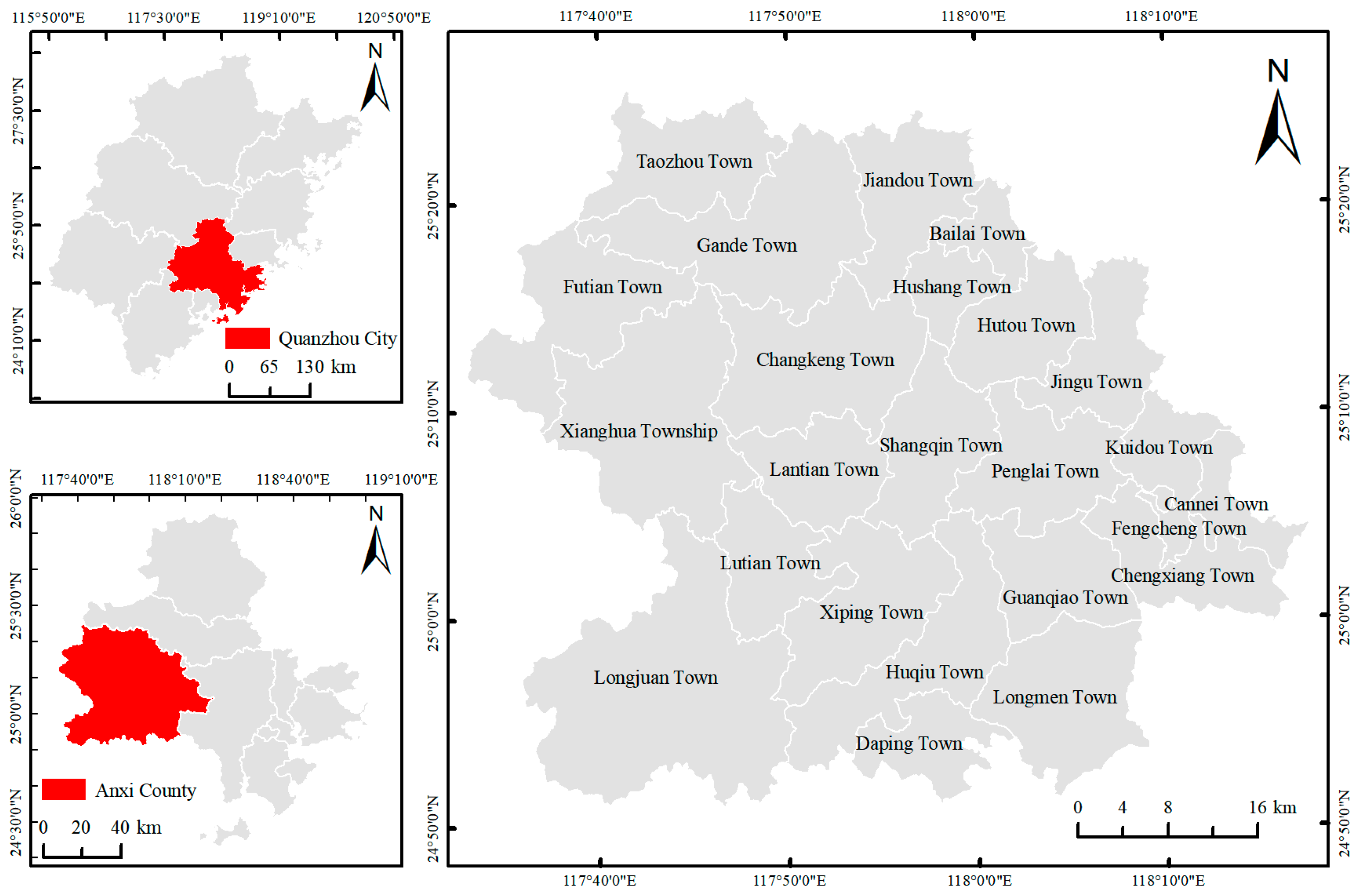
Anxi County is located in the southeastern Fujian Province (117°36′–118°17′ E, 24°50′–25°26′ N) at the headwaters of the West River of the Jinjiang River under the jurisdiction of Quanzhou City, Fujian Province, with a total area of 3057.28 square kilometers, 24 townships, and a total population of over 1.2 million. Anxi County is part of the southeastern extension of the Dayun Mountains, with hilly mountainous terrain and river valley basins featuring a pearl-shaped distribution. The terrain slopes from the northwest to the southeast, featuring undulating mountains, peaks, steep mountains, large slopes, and narrow river valleys in the northwest with an average altitude of 700 m above sea level, a highest peak of 1600 m, and 2461 mountains above 1000 m. In the southeast, the terrain is relatively gentle, with 475 mountains around 1000 m and an average altitude of 500 m or less. The average annual temperature is 16–21 degrees Celsius, and the annual rainfall is 1800 mm, thus forming an excellent area for the growth of Oolong tea, ranking first in China’s key tea-producing counties, known as “China’s tea capital”. Anxi County has a tea plantation area of approx. 60,000 hectares, accounting for around a third of the total area of the tea plantations in Fujian Province, with an annual tea production of 62,000 tons and an industry output value of CNY 32 billion. More than 80% of the population is engaged in tea and related industries, and nearly 60% of the income of tea farmers comes from the tea industry (
Figure 1).
2.2. Data Source and Pre-Processing
The remote sensing image data of the study area were mainly obtained from Landsat/TM/TIRS/OLI released by the Geospatial Data Cloud (
http://www.gscloud.cn (accessed on 16 September 2022). Due to the satellite shooting angle and other factors, the image data were used for three time periods from 2010, 2015, and 2020, with a total of nine image data points, as shown in
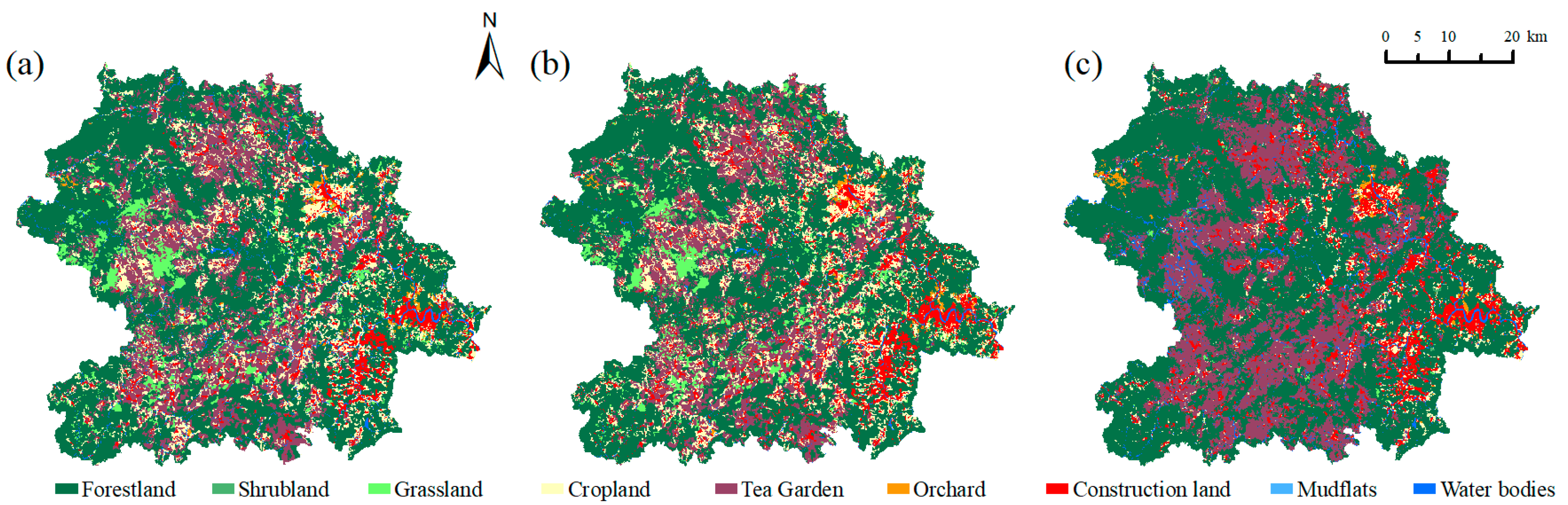
Table 1. The image data of each period were processed using image mosaic, cropping, and correction, converted to true color display using waveband combination, and then compared with Google Earth Pro high-precision historical image data. After the visual interpretation and combination with the field verification and calibration, according to the standard of the National Classification of Land Use Status (GB/721010-2017), combined with the research needs, the maximum likelihood method was used to classify the study area into a total of nine land categories, including forest land, shrubs, grassland, arable land, tea gardens, orchards, construction land (settlements, industrial and mining land, and towns), mudflats, and water bodies. The overall accuracy of the classification of each of these periods was 87.63%, 86.92%, and 88.32%, respectively, to meet the needs of the study. Among them, the data of the tea-related population density in Anxi County and the gross tea product in Anxi County were obtained from the Anxi County Bureau of Statistics, and the uniform projection coordinates and spatial resolution of 30 m were achieved using GIS Kriging interpolation, cropping and resampling operations, and driving-factor data sources (
Table 2,
Figure 2).
2.3. Methods
2.3.1. Selection of Ecosystem Service Functions
Anxi County is one of the important bases for specialized tea areas in China, and the expansion of the tea cultivation scale will have a long-term impact on the provision of ES. Therefore, the selection of the evaluation indicators should first conform to the widely recognized assessment framework, usually based on the Millennium Ecosystem Assessment and the mainstream classification of ecosystem service functions [
40]. Second, in line with the preferences and well-being of the tea plantation stakeholders, the effects of temperature and light on the quality-related metabolites in tea should be considered [
41,
42]. Finally, the availability of the data is important. For this purpose, we selected the water production services, soil conservation services, carbon sequestration services, habitat quality services, and NPP services as the indicators for constructing the CES. Water is one of the basic elements to maintain the growth of tea trees and assessing the water production service can help us understand the contribution of the ecosystem in the study area to maintain the water cycle and water regulation. The soil conservation service aims to provide habitat and nutrient sources for the cultivation of tea trees, reflecting the cycle and supply of soil nutrients in tea plantations and also characterizing the soil erosion in the study area. Woodland was the largest land type in the study area. Therefore, a carbon stock service can help to estimate the carbon stock changes and carbon sink capacity of the study area. Assessing the habitat quality of the study area can reflect its biodiversity changes in different periods. The total plant organic matter reflects the nutrient cycling in the ecosystem and assessing the total plant organic matter can help us understand the ability of the ecosystem for maintaining these ecological processes, such as nutrient cycling.
2.3.2. Ecosystem Service Function Assessment Methods
In this paper, the InVEST model was used to quantitatively estimate the water production services, soil conservation services, carbon sequestration services, and habitat quality services in the study area, and the CASA model was used to quantitatively assess the NPP services [
43]. The water production services were calculated using the water production module of the InVEST model, which is based on the water balance principle, where the actual evapotranspiration is subtracted from the precipitation of each raster to obtain the water production of that raster [
44]. The soil conservation services were calculated using the sediment retention module of the InVEST model [
36]. The parameters were set according to the relevant references. The carbon sequestration service was calculated using the carbon storage module of the InVEST model, and the specific principles and calculation methods are described in [
45]. The average carbon density of the different land types was referred to in relevant studies [
33,
46,
47]. The habitat quality was assessed using the habitat quality module of the InVEST model [
48]. This module reflects the impact of human activities on the environment, and the higher the intensity of human activities, the greater the threat to the habitat [
49,
50]. In this paper, we referred to relevant studies to select arable land, construction land, tea plantations, and orchards as the stressors, and defined woodlands, grasslands, shrubs, mudflats, and water bodies as the habitats [
49]. The NPP services were assessed and calculated using the CASA model since the NPP responds to the total amount of organic matter accumulated by photosynthesis by its green plants per unit area per unit time [
51,
52].
2.3.3. Comprehensive Index for Ecosystem Services
To reflect and quantify the total impact of multiple ecosystem services, a comprehensive index for ecosystem services (CES) was constructed for this paper. In many studies, all the ecosystem services were given equal weights [
53,
54]. However, the importance of the various ecosystem service functions is different. In this paper, based on the previous studies, the CES was constructed using a hierarchical analysis (AHP) [
55] to reflect the overall level of multiple ecosystem services in the study area at different times. The CES was calculated as follows.
where
is the composite ecosystem service index in year
;
is the weight of the
th ecosystem service;
is the normalized value of the ith ecosystem service in year
; and
is the number of ecosystem service types. The AHP was used to determine the weights of each type of ecosystem service (
Table 3).
2.3.4. Factor Selection
The results of numerous studies have shown that both natural environmental factors, such as topography and climate, and socioeconomic factors influence the spatial differentiation of ecosystem service functions. Therefore, it is important to clarify the spatial differentiation of ecosystem service functions and the natural–social and other driving mechanisms for the sustainable development of ecosystem service functions [
56]. Based on the relevant studies and the actual natural–socioeconomic context of the study area, for the representativeness of the selected factors and the availability of data, this study selected the precipitation (PER), temperature (TEM), vegetation cover (NDVI), slope (Slope), elevation (DEM), tea plantation area (T-Area), tea-related population density (T-Pop), and the total tea production value of the study area (T-GDP) as well as another eight representative factors to explore the drivers of the spatial variation in ecosystem service functions [
36,
57].
2.3.5. GWR Model
Ordinary least squares (OLS) models are commonly applied to different regions with related influences [
58]. However, this relationship is assumed to be unchanged across spatial locations. In contrast, a geographically weighted regression, a local regression model, captures the spatial relationships between the dependent and independent variables that vary across locations [
59]. Its equation is as follows.
where
is the dependent variable,
is the
independent variables,
are the geographical coordinates of the
th point;
is the intercept of the
th point,
is the coefficient of
, and
is the residual of the
th point.
A regression equation considering only nearby observations was developed for each point by using the weighted least squares method [
60]. Using various methods, each nearby observation was weighted by a distance function from the regression point. The common spatial weighting or distance decay methods include the fixed Gaussian and adaptive bisquared kernel functions. The fixed Gaussian function can be written as the following.
where
is the weight value of the observation
for estimating the observation coefficient
,
is the distance between
and
, and
is the kernel bandwidth.
The adaptive bisquare function allows the spatial extent to vary at different regression points and includes the same number of adjacent cells for the local model estimation. The formula is as follows.
where
is the adaptive bandwidth. The other variables are the same as in Equation (3).
3. Results
3.1. Ecosystem Services Assessment 2010–2020
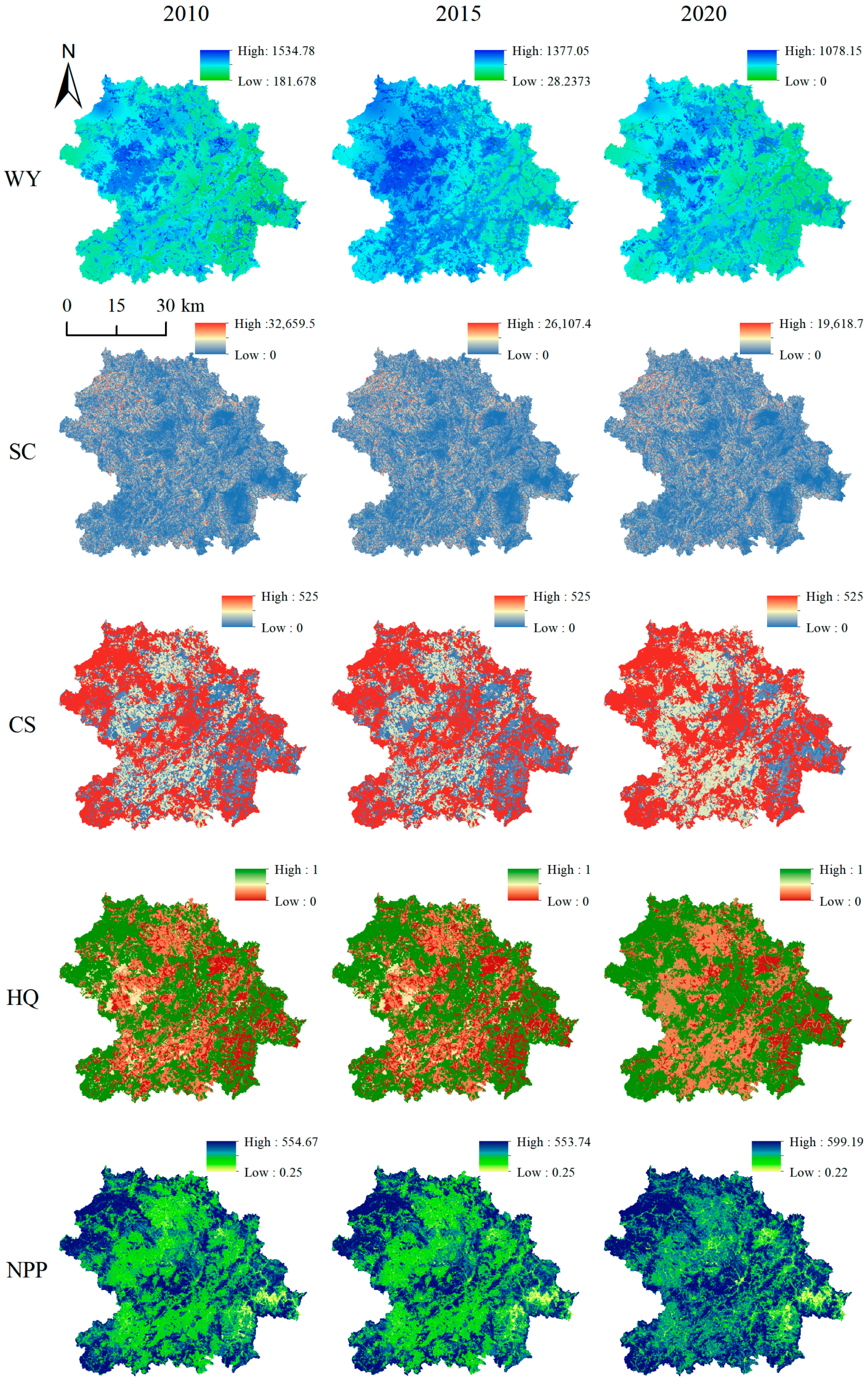
As evaluated by the InVEST model, the results showed (
Figure 3) that from 2010 to 2020 in the study area, the water yield (average water yield depth) was 24.0110 × 10
8 m
3 (803.4045 mm), 24.5233 × 10
8 m
3 (820.3977 mm), and 16.1511 × 10
8 m
3 (540.2287 mm). The water production and the average water production depth both showed a trend of increasing before decreasing. The soil retention was 5.2216 × 10
8 t/ha, 4.3514 × 10
8 t/ha, and 3.3058 × 10
8 t/ha, showing a continuous decreasing trend. The carbon storage was 9.8842 × 10
7 t, 9.7268 × 10
7 t, and 10.1328 × 10
7 t, showing a trend of decreasing and then increasing. The mean values of the habitat quality were 0.6502, 0.6334, and 0.6919, showing a trend of decreasing and then increasing. The mean values of the NPP were 368.2420 gc·m
−2, 371.1052 gc·m
−2, and 448.2230 gc·m
−2, showing a trend of gradually increasing.
3.2. CES Changes from 2010 to 2020
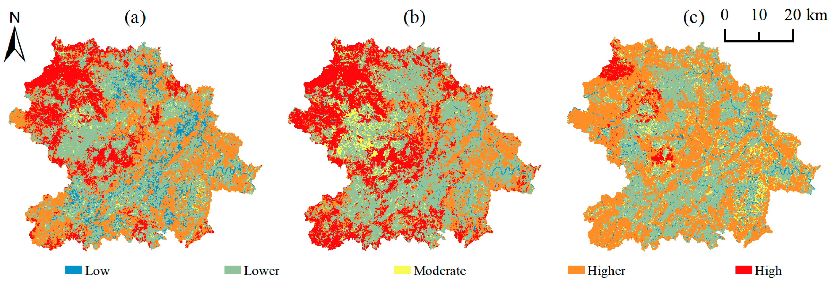
The CES mean value reflects the overall supply state of the ecosystem services, and the CES mean values in the study area from 2010 to 2020 were 0.5398, 0.5763, and 0.5456, in that order. The CES mean values in the study area varied less within each period, showing a trend of increasing and then decreasing. The CES results were divided into five grades: low (0–0.2), lower (0.2–0.4), moderate (0.4–0.6), higher (0.6–0.8), and high (0.8–1). The results showed (
Table 4) that the CES in the study area was high and high grade during the 10 years, and the proportion of the high-grade and low-grade results showed a trend of increasing and then decreasing, while the proportion of the high-grade and low-grade results showed a trend of decreasing and then increasing. The trend of the medium-grade CES results continued to increase while the percentage of the high-grade results decreased by 14.62% and the percentage of the low-grade results decreased by 2.99% (
Figure 4).
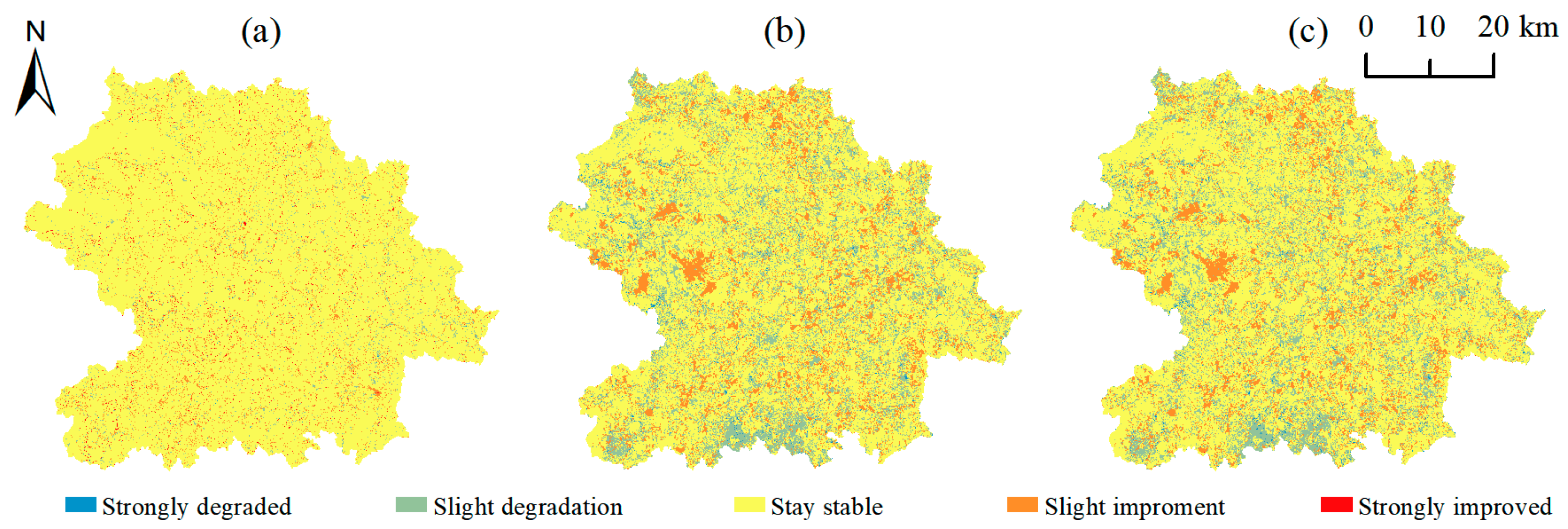
To further explore the spatial and temporal dynamics of the CES in the study area, the CES changes were calculated for each image element and classified into five levels: strongly degraded (−1–−0.5), slight degradation (−0.5–−0.1), stayed stable (−0.1–0.1), slight improvement (0.1–0.5), and strongly improved (0.5–1). As shown in
Table 5 and
Figure 5, most areas of the CES in the study area remained stable during the 10-year period, with an area of 2026.8144 km
2, accounting for 67.81% of the total area of the study area. The area of both the improved and degraded areas showed a continuous increase, with the area of the improved areas being larger than that of degraded areas. The improved areas were mainly concentrated in the western, southwestern, and northeastern parts of the study area, while the degraded areas were mainly distributed in the southeastern and northwestern parts. During the period of 2010–2015, the CES of the study area showed little change, and the area of maintaining a stable grade accounted for 92.36%. However, during the period of 2015–2020, the area and proportion of both the improved and degraded areas of the study area CES increased, with the slightly improved areas being concentrated in the western and eastern regions of the study area while the slightly improved areas were concentrated in the southern region of the study area.
3.3. CES Driver Analysis
The eight selected drivers were fitted with OLS models, and their R2 reached above 0.8. The results indicated that the eight selected drivers could effectively explain the spatial variation in the CES in the study area from 2010 to 2020. However, the OLS model could not spatially present the extent and magnitude of each driver, so this study further combined the application of the GWR model to elucidate the spatial influence of each driver on the ecosystem service function. The results of fitting the OLS model with the GWR model showed that the GWR model fit better than the OLS model, and the GWR model could be used to reveal the spatial distribution of the influence of each driver on the ecosystem service function (
Table 6).
3.3.1. OLS-Based Regression Coefficient Analysis
The
p-value test of the regression coefficients of the OLS model showed that the five drivers of the precipitation, NDVI, DEM, slope, and tea plantation area were highly significantly correlated from 2010–2020. However, the temperature and T-GDP were not correlated. In addition, the T-Pop was not significantly correlated in 2015 (
Table 7).
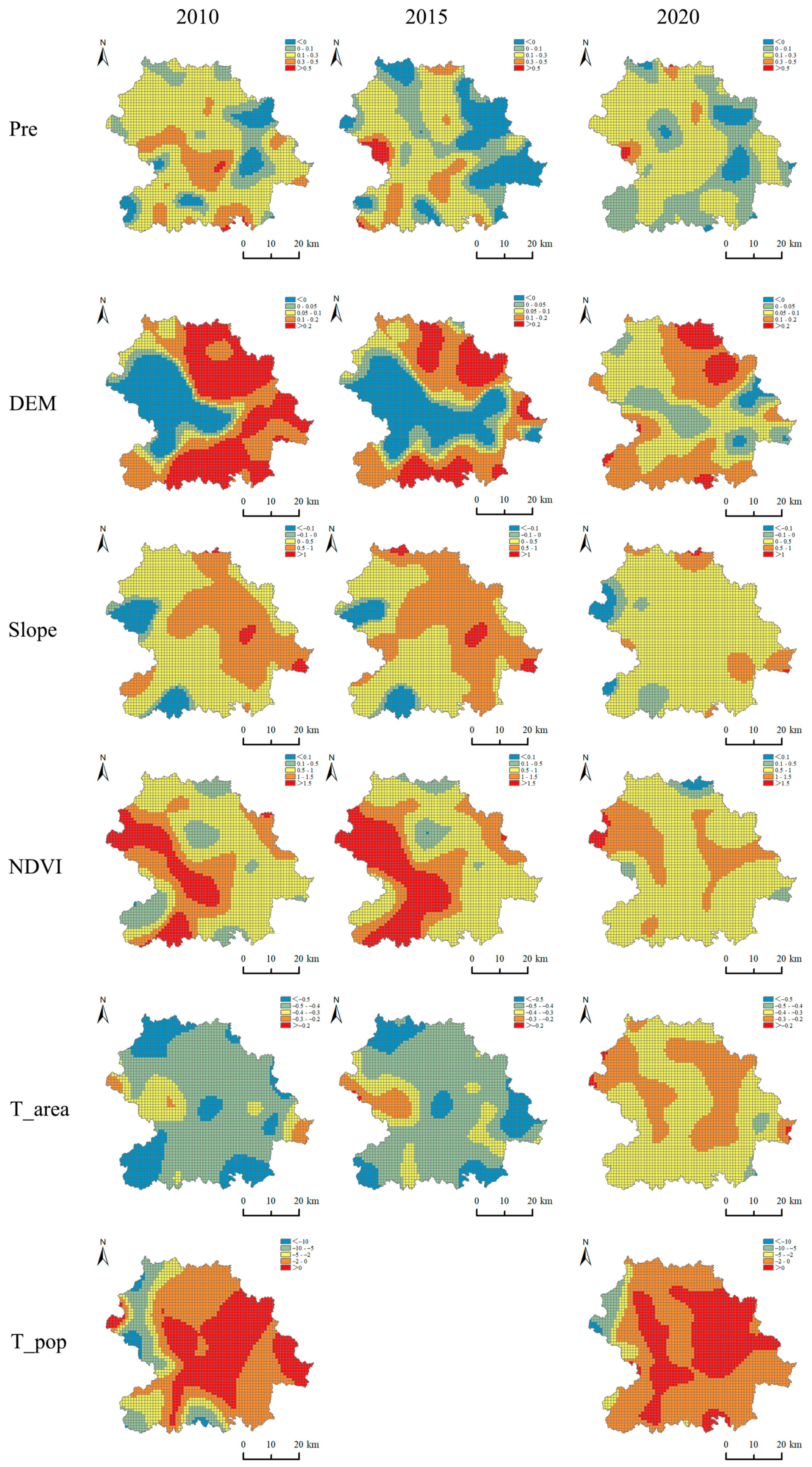
3.3.2. GWR-Based Driver Analysis
The results of the GWR spatial visualization showed that the precipitation, NDVI, DEM, and slope were positively contributed to the CES in most areas of the study area.
The positive promoting effect of the precipitation was mainly concentrated in the western part of the study area, and the influence area gradually decreased with time. The negative inhibition effect was mainly concentrated in the eastern part of the study area, and the negative influence showed a trend of increasing and then decreasing. The reason for the above changes could be that the tea plantations in the western region encroached on the forest land, and the surface capacity to retain water weakened. As the precipitation increased and increased the surface runoff, it caused soil erosion and weakened the CES.
Generally speaking, the higher the elevation, the lower the impact of human activities and the higher the CES. However, in the present study, the positive contribution of the DEM was mainly concentrated in the northeast and south, the significant positive influence area gradually decreased to the northeast region over time, and the negative influence area narrowed and shifted from the west to the east. The reason for the above changes could be that the expansion of tea plantations to higher altitudes has led to the weakening of the positive contribution of the DEM to the CES.
The distribution of the high- and higher-value areas as the second major driver of the positive promoting influence of the slope on the CES showed a trend of first increasing and then sharply decreasing in the eastern region of the study area, gradually shifting to the medium-value area. The negative influencing areas were concentrated in the west and southwest, and the influence range gradually decreased. The reason for the above changes could be that, with the expansion of tea plantations to high-slope areas, the original vegetation cover was changed, which in turn caused the positive contribution of the slope to the CES area to decrease.
The distribution of the NDVI, as the largest driver of the positive contribution of the CES, showed a trend of increasing and then decreasing in the western and southern regions, indicating that the positive contribution of the NDVI to the CES weakened. The reason for the above changes could be that the forest and grassland in the western region were encroached upon by tea plantations, and the original vegetation cover was reduced, which in turn led to a reduction in the positive contribution area of the NDVI.
The tea plantation area and the tea-related population density played a negative inhibitory effect on the CES in most areas of the study area. The higher-value and high-value areas of the negative inhibitory effect of the tea garden area generally changed to the distribution of the medium- and lower-value areas, and the negative inhibitory effect on the CES weakened. Although the area of tea gardens is increasing, with the promotion of green production in tea gardens, ordinary tea gardens have been gradually transformed into ecological tea gardens, and the biodiversity and ecological environment of tea gardens have been improved. Therefore, the negative inhibition of the CES weakened. The positive and negative effects of the tea-related population density on the CES spatially coexisted, and the negative inhibitory effect area decreased, indicating that the negative effect of the tea-related population density on the CES weakened. The reason for the above changes could be that, with the construction of information tea gardens and the rise of tea markets, some tea farmers changed from engaging in tea cultivation to tea management, which reduced the population density engaged in tea cultivation, weakened the impact of human activities on tea gardens, and reduced the negative inhibitory effect areas (
Figure 6).
4. Discussion
- (1)
Impact of the land use type on the CES
Land use is the most important factor that directly affects ecosystem services. With the development of the tea industry economy and rise of the tea market, the regional land use type and distribution pattern with tea as the leading industry has produced significant changes. The disorderly expansion of tea plantations in the study area, high-altitude forest land, low-altitude grassland, and arable land are gradually encroached upon by tea plantations, which affects ecosystem services, such as the water connotation, soil conservation, and carbon sequestration in the study area, causing a series of ecological problems such as soil erosion, reduced vegetation cover, reduced biodiversity, and habitat fragmentation, triggering ecological security. Therefore, it is important to explore the changes in ecosystem services caused by tea plantation expansion to reveal the spatial and temporal evolution patterns of the CES and the main driving factors. The research results provide decision aids for enhancing a regional CES and formulating ecological protection policies.
- (2)
CES drive mechanism
The CES is mainly influenced by the positive promotion of the NDVI and the negative inhibition of the tea garden area. However, the ecosystem service is a whole, and the influence on its overall function is a comprehensive result of multiple factors. The increase or decrease in precipitation directly affects the growth of plants, thus affecting the NDVI, and the level of slope determines the ease of land use development, which determines the reclamation of tea plantations and affects the vegetation cover, thus affecting the ecosystem service function. Meanwhile, related studies showed that the main driving factors affecting the suitability of tea planting and ecosystem service functions in specialized tea areas are the altitude and slope [
61,
62]. This was mainly due to the effect of the elevation and slope on the microclimate of the area, which in turn improves the temperature and precipitation. The NDVI as the response of vegetation to geographic and climatic drivers was the most dominant driver in this study, which laterally illustrated the influence of the geographic environment and climate on the CES. The information construction of tea plantations and the rise of tea markets will not only affect the number of tea farmers but will also adjust the structure of the tea-related population and change the impact of human activities on tea plantations. Therefore, in the exploration of the driving factors of the CES, the correlation between the influencing factors was comprehensively analyzed, which in turn provided the basis for enhancing the CES performance.
- (3)
Shortcomings and Prospects
There were some shortcomings in this study in terms of the selection of the CES drivers. Although two drivers, the tea garden area and the tea-related population density, were innovatively proposed in conjunction with the actual situation of the study area, the mechanism of the policy influence on the spatial variation in the CES was not considered. The driving mechanism of the policy on the spatial variation in the CES should be considered in future studies. The InVEST model was based on a set of simplified assumptions and equations for conducting ecosystem service assessments on a large scale. This simplification may lead to some discrepancies between the model’s results and reality. In addition, the interaction between the tea agro-ecosystem service functions and the surrounding areas should be further explored in future studies.
5. Conclusions
In this study, the InVEST model was applied to assess the ecosystem services in the study area from 2010 to 2020. The mean CES of the study area from 2010 to 2020 was measured and its spatial and temporal evolution characteristics were analyzed. The OLS and GWR models were used to explore the drivers of the spatial and temporal evolution of the CES and the conclusions are as follows.
(1) During the 10 years in the study area, both the water production and average water production depth showed a trend of increasing before decreasing, and the overall water production (average water production depth) decreased by 7.8599 × 10⁸ m3 (263.1758 mm). The soil retention continued to decrease by 1.9158 × 10⁸ t/ha, and the carbon storage showed a trend of decreasing before increasing, with an increase of 0.406 × 10⁷ t. The mean value of the habitat quality showed a trend of decreasing and then increasing, from 0.6502 to 0.6919, and the mean value of the NPP showed a gradual increase, with a total increase of 79.9810 gc·m−2.
(2) The mean value of the CES in the study area from 2010 to 2020 showed a trend of increasing and then decreasing, with an overall increasing trend from 0.5398 to 0.5456. The proportion of the high-value area to the lower-value area in the study area during the 10-year period showed a trend of increasing and then decreasing, and the proportion of the higher-value area to the lower-value area showed a trend of decreasing and then increasing. The changes in the spatial characteristics of the CES maintained the largest area of stable grade. The area of both the improved and degraded areas showed a continuous increasing trend, and the area of the improved areas was larger than that of degraded areas. The improved areas were mainly concentrated in the west, southwest, and northeast of the study area, and the degraded areas were mainly distributed in the southeast and northwest.
(3) The OLS correlation coefficients indicated that the precipitation, NDVI, DEM, and slope positively contributed to the CES. The correlation coefficients of the precipitation, NDVI, and slope decreased and the positive contribution weakened, while the correlation coefficients of the DEM and slope increased and the positive contribution increased. However, the correlation coefficient values of the precipitation, NDVI, and slope decreased and the positive contribution weakened, while the correlation coefficient values of the DEM and slope increased. The negative inhibition effect of the tea plantation area and the tea-related population density weakened over the study period.
(4) The main drivers of the spatial variation in the CES were the NDVI (0.8986–0.6913) and the tea plantation area (−0.4911–−0.3228). The high values of the positive contribution of the NDVI were mainly concentrated in the western and southern regions, showing an increasing and then decreasing trend, and indicated that the positive contribution of the NDVI to the CES weakened. The high value of the negative inhibition of the tea garden area was mainly distributed in the northern and southern regions, showing a decreasing trend and indicated that the negative inhibition effect of the tea garden area on the CES weakened.
Author Contributions
Conceptualization, W.L. (Wen Li); methodology, W.L. (Wen Li), S.F. and J.G.; software, J.G. and J.B.; validation, W.L. (Wenxiong Lin) and S.F.; formal analysis, W.L. (Wen Li) and S.F.; investigation, J.G. and J.B.; resources, J.G.; data curation, W.L. (Wen Li) and W.L. (Wenxiong Lin); writing—original draft preparation, W.L. (Wen Li); writing—review and editing, S.F.; visualization, W.L. (Wen Li), J.G. and J.B.; supervision, S.F. and Z.W.; project administration, S.F.; funding acquisition, S.F. All authors have read and agreed to the published version of the manuscript.
Funding
This work was supported by the Fujian Agriculture and Forestry University Tea Industry Chain Science and Technology Innovation Team Project: Tea Industry Economy and Creativity Research (K1520012A08), the Science and Education Special Project of Fujian Province: Science and Technology Integration and Mechanism of “Small Industrial Courtyard” for Special Modern Agriculture (K8120K01a), the Fujian Agriculture and Forestry University’s “industry creation integration” talent training practice platform construction based on industrial revitalization of tea economy (111420049), and the Leisure agriculture and industry integration service team (11899170121).
Institutional Review Board Statement
Not applicable.
Informed Consent Statement
Not applicable.
Data Availability Statement
The data that support the findings of this study are available from the authors upon reasonable request.
Conflicts of Interest
The authors declare no conflict of interest.
References
- Storkey, J.; Döring, T.; Baddeley, J.; Collins, R.; Roderick, S.; Jones, H.; Watson, C. Engineering a plant community to deliver multiple ecosystem services. Ecol. Appl. 2015, 25, 1034–1043. [Google Scholar]
- Tianhong, L.; Wenkai, L.; Zhenghan, Q. Variations in ecosystem service value in response to land use changes in Shenzhen. Ecol. Econ. 2010, 69, 1427–1435. [Google Scholar]
- Bennett, E.M.; Peterson, G.D.; Gordon, L.J. Understanding relationships among multiple ecosystem services. Ecol. Lett. 2009, 12, 1394–1404. [Google Scholar]
- Liu, H.; Xiao, W.; Li, Q.; Tian, Y.; Zhu, J. Spatio-temporal change of multiple ecosystem services and their driving factors: A case study in Beijing, China. Forests 2022, 13, 260. [Google Scholar]
- Biao, Z.; Yunting, S.; Shuang, W. A review on the driving mechanisms of ecosystem services change. J. Resour. Ecol. 2022, 13, 68–79. [Google Scholar]
- Kumar, M.; Kumar, P. Valuation of the ecosystem services: A psycho-cultural perspective. Ecol. Econ. 2008, 64, 808–819. [Google Scholar]
- De Groot, R.S.; Fisher, B.; Christie, M.; Aronson, J.; Braat, L.; Haines-Young, R.; Gowdy, J.; Maltby, E.; Neuville, A.; Polasky, S. Integrating the ecological and economic dimensions in biodiversity and ecosystem service valuation. In The Economics of Ecosystems and Biodiversity (TEEB): Ecological and Economic Foundations; Earthscan, Routledge: London, UK, 2010; pp. 9–40. [Google Scholar]
- Wolff, S.; Schulp, C.; Verburg, P.H. Mapping ecosystem services demand: A review of current research and future perspectives. Ecol. Indic. 2015, 55, 159–171. [Google Scholar]
- Potschin, M.B.; Haines-Young, R.H. Ecosystem services: Exploring a geographical perspective. Prog. Phys. Geogr. 2011, 35, 575–594. [Google Scholar]
- Haase, D.; Larondelle, N.; Andersson, E.; Artmann, M.; Borgström, S.; Breuste, J.; Gomez-Baggethun, E.; Gren, Å.; Hamstead, Z.; Hansen, R. A quantitative review of urban ecosystem service assessments: Concepts, models, and implementation. Ambio 2014, 43, 413–433. [Google Scholar]
- Marino, D.; Palmieri, M.; Marucci, A.; Tufano, M. Comparison between demand and supply of some ecosystem services in national parks: A spatial analysis conducted using Italian case studies. Conservation 2021, 1, 36–57. [Google Scholar]
- Sanon, S.; Hein, T.; Douven, W.; Winkler, P. Quantifying ecosystem service trade-offs: The case of an urban floodplain in Vienna, Austria. J. Environ. Manag. 2012, 111, 159–172. [Google Scholar] [CrossRef] [PubMed]
- Mouchet, M.A.; Lamarque, P.; Martín-López, B.; Crouzat, E.; Gos, P.; Byczek, C.; Lavorel, S. An interdisciplinary methodological guide for quantifying associations between ecosystem services. Glob. Environ. Change 2014, 28, 298–308. [Google Scholar] [CrossRef]
- Benra, F.; De Frutos, A.; Gaglio, M.; Álvarez-Garretón, C.; Felipe-Lucia, M.; Bonn, A. Mapping water ecosystem services: Evaluating InVEST model predictions in data scarce regions. Environ. Modell. Softw. 2021, 138, 104982. [Google Scholar] [CrossRef]
- Villa, F.; Ceroni, M.; Bagstad, K.; Johnson, G.; Krivov, S. ARIES (Artificial Intelligence for Ecosystem Services): A new tool for ecosystem services assessment, planning, and valuation. In Proceedings of the 11th Annual BIOECON Conference on Economic Instruments to Enhance the Conservation and Sustainable Use of Biodiversity, Venice, Italy, 21–22 September 2009. [Google Scholar]
- Li, P.; Zhang, R.; Xu, L. Three-dimensional ecological footprint based on ecosystem service value and their drivers: A case study of Urumqi. Ecol. Indic. 2021, 131, 108117. [Google Scholar] [CrossRef]
- Kumar, R.; Mishra, A.; Jha, B. Bacterial community structure and functional diversity in subsurface seawater from the western coastal ecosystem of the Arabian Sea, India. Gene 2019, 701, 55–64. [Google Scholar] [CrossRef]
- Kim, I.; Arnhold, S.; Ahn, S.; Le, Q.B.; Kim, S.J.; Park, S.J.; Koellner, T. Land use change and ecosystem services in mountainous watersheds: Predicting the consequences of environmental policies with cellular automata and hydrological modeling. Environ. Modell. Softw. 2019, 122, 103982. [Google Scholar] [CrossRef]
- Zhao, Q.; Li, J.; Liu, J.; Cuan, Y.; Zhang, C. Integrating supply and demand in cultural ecosystem services assessment: A case study of Cuihua Mountain (China). Environ. Sci. Pollut. Res. 2019, 26, 6065–6076. [Google Scholar] [CrossRef]
- Grafius, D.R.; Corstanje, R.; Warren, P.H.; Evans, K.L.; Hancock, S.; Harris, J.A. The impact of land use/land cover scale on modelling urban ecosystem services. Landsc. Ecol. 2016, 31, 1509–1522. [Google Scholar] [CrossRef]
- Yang, J.; Xie, B.; Tao, W.; Zhang, D. Ecosystem Services Assessment, Trade-Off, and Bundles in the Yellow River Basin, China. Diversity 2021, 13, 308. [Google Scholar] [CrossRef]
- Redhead, J.W.; Stratford, C.; Sharps, K.; Jones, L.; Ziv, G.; Clarke, D.; Oliver, T.H.; Bullock, J.M. Empirical validation of the InVEST water yield ecosystem service model at a national scale. Sci. Total Environ. 2016, 569, 1418–1426. [Google Scholar] [CrossRef]
- Xiao, F.; Liu, Q.; Xu, Y. Estimation of Terrestrial Net Primary Productivity in the Yellow River Basin of China Using Light Use Efficiency Model. Sustainability 2022, 14, 7399. [Google Scholar] [CrossRef]
- De Groot, R.S.; Wilson, M.A.; Boumans, R.M. A typology for the classification, description and valuation of ecosystem functions, goods and services. Ecol. Econ. 2002, 41, 393–408. [Google Scholar] [CrossRef]
- Wang, J.; Zhou, W.; Pickett, S.T.; Yu, W.; Li, W. A multiscale analysis of urbanization effects on ecosystem services supply in an urban megaregion. Sci. Total Environ. 2019, 662, 824–833. [Google Scholar] [CrossRef] [PubMed]
- Canedoli, C.; Ferrè, C.; El Khair, D.A.; Comolli, R.; Liga, C.; Mazzucchelli, F.; Proietto, A.; Rota, N.; Colombo, G.; Bassano, B. Evaluation of ecosystem services in a protected mountain area: Soil organic carbon stock and biodiversity in alpine forests and grasslands. Ecosyst. Serv. 2020, 44, 101135. [Google Scholar] [CrossRef]
- Wang, Z.; Lechner, A.M.; Yang, Y.; Baumgartl, T.; Wu, J. Mapping the cumulative impacts of long-term mining disturbance and progressive rehabilitation on ecosystem services. Sci. Total Environ. 2020, 717, 137214. [Google Scholar] [CrossRef]
- Carpenter, S.R.; Mooney, H.A.; Agard, J.; Capistrano, D.; DeFries, R.S.; Díaz, S.; Dietz, T.; Duraiappah, A.K.; Oteng-Yeboah, A.; Pereira, H.M. Science for managing ecosystem services: Beyond the Millennium Ecosystem Assessment. Proc. Natl. Acad. Sci. USA 2009, 106, 1305–1312. [Google Scholar] [CrossRef]
- Häyhä, T.; Franzese, P.P. Ecosystem services assessment: A review under an ecological-economic and systems perspective. Ecol. Model. 2014, 289, 124–132. [Google Scholar] [CrossRef]
- Kim, S.; Jung, Y. Application of the InVEST model to quantify the water yield of North Korean forests. Forests 2020, 11, 804. [Google Scholar] [CrossRef]
- Sallustio, L.; De Toni, A.; Strollo, A.; Di Febbraro, M.; Gissi, E.; Casella, L.; Geneletti, D.; Munafò, M.; Vizzarri, M.; Marchetti, M. Assessing habitat quality in relation to the spatial distribution of protected areas in Italy. J. Environ. Manag. 2017, 201, 129–137. [Google Scholar] [CrossRef]
- Wang, B.; Cheng, W. Effects of land use/cover on regional habitat quality under different geomorphic types based on InVEST model. Remote Sens. 2022, 14, 1279. [Google Scholar] [CrossRef]
- Zhao, M.; He, Z.; Du, J.; Chen, L.; Lin, P.; Fang, S. Assessing the effects of ecological engineering on carbon storage by linking the CA-Markov and InVEST models. Ecol. Indic. 2019, 98, 29–38. [Google Scholar] [CrossRef]
- Ding, Q.; Chen, Y.; Bu, L.; Ye, Y. Multi-scenario analysis of habitat quality in the Yellow River delta by coupling FLUS with InVEST model. Int. J. Environ. Res. Public Health 2021, 18, 2389. [Google Scholar] [CrossRef] [PubMed]
- He, Y.; Ma, J.; Zhang, C.; Yang, H. Spatio-Temporal Evolution and Prediction of Carbon Storage in Guilin Based on FLUS and InVEST Models. Remote Sens. 2023, 15, 1445. [Google Scholar] [CrossRef]
- Reheman, R.; Kasimu, A.; Duolaiti, X.; Wei, B.; Zhao, Y. Research on the Change in Prediction of Water Production in Urban Agglomerations on the Northern Slopes of the Tianshan Mountains Based on the InVEST-PLUS Model. Water 2023, 15, 776. [Google Scholar] [CrossRef]
- Wang, C.; Li, T.; Guo, X.; Xia, L.; Lu, C.; Wang, C. Plus-InVEST Study of the Chengdu-Chongqing urban agglomeration’s land-use change and carbon storage. Land 2022, 11, 1617. [Google Scholar] [CrossRef]
- Sylla, M.; Hagemann, N.; Szewrański, S. Mapping trade-offs and synergies among peri-urban ecosystem services to address spatial policy. Environ. Sci. Policy 2020, 112, 79–90. [Google Scholar] [CrossRef]
- Lin, S.; Wu, R.; Yang, F.; Wang, J.; Wu, W. Spatial trade-offs and synergies among ecosystem services within a global biodiversity hotspot. Ecol. Indic. 2018, 84, 371–381. [Google Scholar] [CrossRef]
- Bai, Y.; Chen, Y.; Alatalo, J.M.; Yang, Z.; Jiang, B. Scale effects on the relationships between land characteristics and ecosystem services-a case study in Taihu Lake Basin, China. Sci. Total Environ. 2020, 716, 137083. [Google Scholar] [CrossRef]
- Wang, M.; Yang, J.; Li, J.; Zhou, X.; Xiao, Y.; Liao, Y.; Tang, J.; Dong, F.; Zeng, L. Effects of temperature and light on quality-related metabolites in tea [Camellia sinensis (L.) Kuntze] leaves. Food Res. Int. 2022, 161, 111882. [Google Scholar] [CrossRef]
- Wen, X.; Zhang, Z.; Huang, X. Heavy metals in karst tea garden soils under different ecological environments in southwestern China. Trop. Ecol. 2022, 63, 495–505. [Google Scholar] [CrossRef]
- Feng, X.; Zhang, T.; Feng, P.; Li, J. Evaluation and tradeoff-synergy analysis of ecosystem services in Luanhe River Basin. Ecohydrology 2022, 15, e2473. [Google Scholar] [CrossRef]
- Xiu, Y.; Wang, N.; Liu, S.; Guo, Z.; Peng, F. Impact of Agricultural Use of Sand Land on Water Yield Services under Different Development Intensities in the Agro-Pastoral Ecotone of Northern Shaanxi. Geofluids 2022, 2022, 1678442. [Google Scholar] [CrossRef]
- Pais, S.; Aquilué, N.; Campos, J.; Sil, Â.; Marcos, B.; Martínez-Freiría, F.; Domínguez, J.; Brotons, L.; Honrado, J.P.; Regos, A. Mountain farmland protection and fire-smart management jointly reduce fire hazard and enhance biodiversity and carbon sequestration. Ecosyst. Serv. 2020, 44, 101143. [Google Scholar] [CrossRef]
- Fang, J.; Yang, Y.; Ma, W.; Mohammat, A.; Shen, H. Ecosystem carbon stocks and their changes in China’s grasslands. Sci. China Life Sci. 2010, 53, 757–765. [Google Scholar] [CrossRef]
- Guo, Z.; Hu, H.; Li, P.; Li, N.; Fang, J. Spatio-temporal changes in biomass carbon sinks in China’s forests from 1977 to 2008. Sci. China Life Sci. 2013, 56, 661–671. [Google Scholar] [CrossRef]
- Xiao, P.; Zhou, Y.; Li, M.; Xu, J. Spatiotemporal patterns of habitat quality and its topographic gradient effects of Hubei Province based on the InVEST model. Environ. Dev. Sustain. 2022, 25, 6419–6448. [Google Scholar] [CrossRef]
- Wu, L.; Sun, C.; Fan, F. Estimating the characteristic spatiotemporal variation in habitat quality using the invest model—A case study from Guangdong-Hong Kong-Macao Greater Bay Area. Remote Sens. 2021, 13, 1008. [Google Scholar] [CrossRef]
- De Groot, R.S.; Alkemade, R.; Braat, L.; Hein, L.; Willemen, L. Challenges in integrating the concept of ecosystem services and values in landscape planning, management and decision making. Ecol. Complex. 2010, 7, 260–272. [Google Scholar] [CrossRef]
- Field, C.B.; Randerson, J.T.; Malmström, C.M. Global net primary production: Combining ecology and remote sensing. Remote Sens. Environ. 1995, 51, 74–88. [Google Scholar] [CrossRef]
- Potter, C.S.; Randerson, J.T.; Field, C.B.; Matson, P.A.; Vitousek, P.M.; Mooney, H.A.; Klooster, S.A. Terrestrial ecosystem production: A process model based on global satellite and surface data. Glob. Biogeochem. Cycle 1993, 7, 811–841. [Google Scholar] [CrossRef]
- Liu, S.; Crossman, N.D.; Nolan, M.; Ghirmay, H. Bringing ecosystem services into integrated water resources management. J. Environ. Manag. 2013, 129, 92–102. [Google Scholar] [CrossRef] [PubMed]
- Watson, K.B.; Galford, G.L.; Sonter, L.J.; Koh, I.; Ricketts, T.H. Effects of human demand on conservation planning for biodiversity and ecosystem services. Conserv. Biol. 2019, 33, 942–952. [Google Scholar] [CrossRef] [PubMed]
- Arellanos, E.; Guzman, W.; García, L. How to Prioritize the Attributes of Water Ecosystem Service for Water Security Management: Choice Experiments versus Analytic Hierarchy Process. Sustainability 2022, 14, 15767. [Google Scholar] [CrossRef]
- Fang, L.; Wang, L.; Chen, W.; Sun, J.; Cao, Q.; Wang, S.; Wang, L. Identifying the impacts of natural and human factors on ecosystem service in the Yangtze and Yellow River Basins. J. Clean Prod. 2021, 314, 127995. [Google Scholar] [CrossRef]
- Pan, N.; Guan, Q.; Wang, Q.; Sun, Y.; Li, H.; Ma, Y. Spatial differentiation and driving mechanisms in ecosystem service value of arid region: A case study in the middle and lower reaches of Shule River Basin, NW China. J. Clean Prod. 2021, 319, 128718. [Google Scholar] [CrossRef]
- Zhu, C.; Zhang, X.; Zhou, M.; He, S.; Gan, M.; Yang, L.; Wang, K. Impacts of urbanization and landscape pattern on habitat quality using OLS and GWR models in Hangzhou, China. Ecol. Indic. 2020, 117, 106654. [Google Scholar] [CrossRef]
- Huang, Z.; Li, S.; Peng, Y.; Gao, F. Spatial Non-Stationarity of Influencing Factors of China’s County Economic Development Base on a Multiscale Geographically Weighted Regression Model. ISPRS Int. J. Geo-Inf. 2023, 12, 109. [Google Scholar] [CrossRef]
- Ruppert, D.; Wand, M.P. Multivariate locally weighted least squares regression. Ann. Stat. 1994, 22, 1346–1370. [Google Scholar] [CrossRef]
- Guo, X.; Min, Q. Analysis of Landscape Patterns Changes and Driving Factors of the Guangdong Chaoan Fenghuangdancong Tea Cultural System in China. Sustainability 2023, 15, 5560. [Google Scholar] [CrossRef]
- Chen, P.; Li, C.; Chen, S.; Li, Z.; Zhang, H.; Zhao, C. Tea Cultivation Suitability Evaluation and Driving Force Analysis Based on AHP and Geodetector Results: A Case Study of Yingde in Guangdong, China. Remote Sens. 2022, 14, 2412. [Google Scholar] [CrossRef]
| Disclaimer/Publisher’s Note: The statements, opinions and data contained in all publications are solely those of the individual author(s) and contributor(s) and not of MDPI and/or the editor(s). MDPI and/or the editor(s) disclaim responsibility for any injury to people or property resulting from any ideas, methods, instructions or products referred to in the content. |
© 2023 by the authors. Licensee MDPI, Basel, Switzerland. This article is an open access article distributed under the terms and conditions of the Creative Commons Attribution (CC BY) license (https://creativecommons.org/licenses/by/4.0/).


