Abstract
The knowledge of temporal variability of soil hydraulic properties (SHPs) in agricultural fields can help in reliable assessment of crop water requirement, thus improving irrigation water usage efficiency. The Fokker–Planck equation (FPE) and its modified forms are popularly used to describe temporal variation in SHPs. These models consider statistical description of soil pore size distribution (PSD) as a probability density function to estimate SHP evolution with time. In this study, we compare four different models to describe the temporal evolution of PSD and SHPs for multiple datasets across the world with different soil types, tillage conditions and crop cover. Further, field experiments were carried out at an experimental agricultural field at IIT Kanpur for rice crops, and the performance of these models was also evaluated for Indian conditions. It is observed that existing models have low accuracy for small pore radii values, and the prediction ability of these models is more affected by soil type rather than tillage conditions. More observations can improve the performance of FPE-based numerical and analytical models. The POWER Model is the least accurate because of its inherent power law assumption of PSD, which results in incorrect values for low pore radii. The FPE analytical model can be reliably used for predicting PSD and SHP evolution at most of the field sites.
1. Introduction
Sustainable management of water resources in an agricultural field requires an accurate assessment of water demand as well as losses. Soil plays an important role in this by not only allowing water and nutrient extraction by roots but also by providing physical support for crop growth [1]. The overall goal of various agricultural management practices, such as tillage, crop rotation, and cropping patterns, is to create optimum characteristics for crop growth and minimize environmental degradation, as well as to optimize water use [2]. Soil hydraulic properties (SHPs) have a significant role in this. SHPs refer to the soil water retention function and the hydraulic conductivity function where and are moisture content, hydraulic conductivity, and suction head, respectively [2,3,4]. The indicates the ability of the soil to hold and retain water while governs the movement of water and solute through the unsaturated zone. SHPs not only govern water movement but also affect plant water and nutrient uptake, thus influencing the dynamics of various hydrological and biological processes within the unsaturated zone [5,6].
SHPs depend upon soil texture, structure, presence of organic matter and chemical and biological properties of the soil. Soil structure-dependent properties are highly dynamic and change with time and depth due to various agronomic practices and environmental factors [7,8]. Various studies have shown that soil physical properties that depend on soil structure, such as moisture content, bulk density, macro-porosity, saturated and near-saturated hydraulic conductivity etc., are heavily influenced by seasonal changes in climate and climate-induced pedological factors [7,9,10]. Furthermore, various researchers have observed that significant changes in soil structure are caused by different soil and crop management practices [11,12,13,14,15,16,17,18]. A common observation from these studies is that the temporal variability of SHPs exceeds the variability induced by crops, tillage, or land use.
These above-mentioned studies have quantified the temporal variation in SHPs, but the findings of these studies are site-specific and vary depending on the climate, soil type, measurement technique and sampling strategy. Furthermore, the SHP measurements in most of the studies have been done at only a few time intervals and have been restricted to the surface soil layer during the study duration.
The SHPs significantly affect various hydrological processes, e.g., evapotranspiration, surface runoff, infiltration, and groundwater recharge. A few studies have looked at the effect of temporal variation in SHP on water movement in agricultural fields. The authors of [19] studied the effect of time-dependent hydraulic conductivity on water flow simulations for an experimental plot located in China under different tillage practices and Maize crop cover. They observed that the incorporation of time-varying hydraulic conductivity improved estimates of percolation losses by 6% under wetting conditions and of water storage by 13–14%. In addition, improvement in estimates of evaporation and transpiration losses was also observed. The authors of [13] investigated the effect of incorporating time-variable SHPs in a soil water simulation and compared the results against measured data for different tillage methods in the near-surface soil profile (0–30 cm). They observed that the inclusion of temporal variability of SHPs led to significant improvement in the performance of the model for all treatments, resulting in average relative errors of less than 13%. Another study [6] attempted to characterize the temporal variation in SHP for an experimental maize plot and analyzed the effect of considering temporally varying SHPs against constant SHPs on simulations of water movement. The incorporation of time-varying SHPs significantly improved soil water predictions up to a 30 cm depth. Another team [20] investigated the temporal and spatial variability of SHPs during a cropping cycle between April and September 2015 for a surface-irrigated maize field in northern Italy and quantified the effect of SHPs on simulations of soil water movement using the FEST- WB model. They observed that a well-parameterized model that accounts for spatiotemporal variation in SHPs improved the accuracy of simulations. Similar observations were made by the authors of [21] in an uncultivated Fluvisol field by using both in situ and laboratory measurements. Recently, the authors of [18] investigated the effect of incorporating seasonal variability of SHPs in hydrological models. They observed the significant impact of the inclusion of short-term temporal variability of SHPs on soil-water dynamics for both ploughed and no-till (NT) condition. Variations up to 44% were observed when the water content was modeled based on SHPs calculated using multiple sampling events vs. that from single sampling events. They postulated that neglecting temporal variability in a hydrological model might lead to an underestimation of the extreme values in a simulation.
The above-mentioned studies highlight the need to incorporate temporal variability in SHPs to improve the simulation of water movement in agricultural fields; however, it is worth noting that SHPs are still considered constant in most of the modeling studies.
In the last two decades, limited efforts have been directed towards investigating the temporal dynamics of SHP [5,6,13,16,17,22,23]. Predictive models for SHPs can be developed using the statistical description of soil pore space as a probability density function (PDF) [24,25,26,27,28]. The authors of [24] proposed a stochastic modeling framework to describe the temporal variability of soil PSD. The Fokker–Planck equation (FPE) was used to combine the probabilistic nature of PSD along with physically based soil deformation models to account for the dynamics of the mean soil pore radius and its variance, as well as total porosity. Using the numerical solution of FPE, they modeled the changes in soil PSD due to the wetting—drying cycles and the resultant Soil Water Retention Curve (SWRC) and . The initial soil PSD was taken as lognormal.
Another study [25] presented two analytical solutions for modeling PSD evolution as per the modeling framework presented by the authors of [24]. For the first solution, it was assumed that the drift and degradation coefficients depend on time; however, for the second solution, both were dependent on pore size as well as time. Both solutions were applied to model the soil PSD evolution for Millville silt loam soil. The predicted soil PSD was used to obtain , which was found to be in good agreement with experimental data. The initial soil PSD was taken as a lognormal distribution. A further attempt was made by [26] to present an analytical solution for the PSD for the case where drift and degradation coefficients depend on time, and the dispersion coefficients are proportional to the drift coefficients. These coefficients could be estimated from PSD or SWRC data as well as those from mechanistic models.
Following previous work by the authors of [24,25,26], an alternate modeling framework was proposed to describe the temporal evolution of the PSD while considering processes such as tillage, consolidation, and changes in organic matter [28]. Instead of FPE, a modified transport equation was used that neglected the diffusion term and a time-varying power-law PSD was obtained as the solution. The obtained solution is different from earlier studies and has a clear connection to well-known power law for SWRC [29,30]. They derived expressions for soil properties from the model and linked its parameters to soil processes and management activities such as tillage, soil consolidation, and changes in SOM. It was found that the model in this study accurately captured the physical consistency of key soil parameters as they changed with soil biogeochemistry over time and exhibited realistic patterns. It was noted that the proposed model did not account for very short-term changes in soil properties, such as those due to wetting and drying cycles.
The proposed numerical and analytical models attempt to quantify management-induced changes in soil structure and incorporate these results into mathematical functions describing temporal changes in the PSD. They can improve our capacity to assess the overall impacts of different soil and crop management practices on soil physical properties and water balance. However, as of now, the full potential of these models in predicting the temporal variation in SHPs is yet to be explored.
The authors of [31] attempted to characterize the alteration in soil structure due to a crop–pasture rotation at an experimental site at Lincoln University. The measurement results were incorporated into the analytical models proposed in [25,26]. It was observed that the adapted pore size evolution model was suitable for predicting management-induced changes in soil structure. However, a reasonable agreement between the measured and predicted PSD was obtained only when an assumed time-dependent degradation of pores was incorporated into the model. The authors of [32] investigated the effect of crop species with different root systems on field soil pore properties. They conducted a field experiment with twelve species from different families. The parameters of Kosugi’s PSD model were determined inversely from the tension infiltrometer data. The measured root traits were related to pore variables by regression analysis. Then, they used the FPE solution proposed by [25,26] to analyze if observed pore dynamics followed a diffusion-like process. However, they observed that the diffusion-type pore evolution model could only partially capture the observed PSD dynamics.
The authors of [2] reviewed various studies related to the temporal dynamics of SHPs. They applied the analytical solution of FPE found in [25,26] to two SWRC datasets available in the literature to evaluate its suitability to predict the evolution of soil PSD following tillage as well as when there is a change in tillage regime. They observed that the model performed better for change in tillage regimes as compared to the seasonal evolution of soil PSD. Another study [3] further investigated the applicability of the model in [24,25] in terms of the retention data obtained from various studies for different tillage treatments across the globe. The datasets were categorized for two cases: (a) for change in tillage regime and (b) for the temporal dynamics of soil pore space in the months following tillage. They observed that the model provides a reasonable fit. Further, they observed that the applicability of the model was limited due to the lack of adequate datasets for different management practices, soil types, and climate regimes. The availability of such data can be used in calibrating and including new coefficients and sink/source terms for the model.
While the above studies provide useful insight into the performance of the FPE-based models [24,25,26], none of the existing studies have evaluated the performance of all the existing models for a common dataset. Therefore, the prime objective of this study is to perform comparison studies for different models to describe the temporal evolution of soil PSD and, subsequently, the soil hydraulic properties.
2. Governing Equations and Models
In this section, we briefly describe FPE, and the modified transport equation used to describe the time-evolution of the soil PSD.
2.1. Fokker–Planck Equation
The FPE solution describes the evolution of the probability density function (PDF) for the attribute [24]. FPE has been used to model the PDF associated with stochastic processes. Representation of soil PSD in terms of statistical PDF and considering aggregate deformation and porosity loss in wet soils as a solid diffusion process enables modeling soil pore space changes as the evolution of soil PSD is governed by external forcing and soil deformation processes [24].
The FPE is given as follows:
where is the PSD, is the drift coefficient or the infinitesimal mean, is the diffusion coefficient or the infinitesimal variance, and is the source/sink term or first-order pore degradation factor representing instantaneous pore loss . The terms and refer to pore radius and time , respectively. The application of FPE to modeling PSD evolution was also motivated by its similarity with the advection-dispersion equation and a similar decay term that may allow the use of existing analytical solutions. The boundary conditions of the above equation used are.
with as the initial PSD. The lower boundary condition stipulates a zero-probability flux, i.e., pores cannot assume a negative radius. To ensure the conservation, the upper boundary condition requires a zero gradient, i.e., a zero-probability flux for infinitely large pores. The homogeneous zero flux conditions imply that any loss of probability (PSD) is due to degradation. The coefficients and can be obtained as defined in [32].
The mean change in pore radius and the variance of changes in pore radii with time are represented by and respectively. The moments are defined by integrating the PSD with respect to the pore radius.
For example, a zero-order moment is given as:
Normalized moments are calculated through the division of by . The first-order normalized moment characterizes the mean pore size and the second-order centralized moment characterizes the variance and they can be obtained as:
can be obtained by:
The cumulative drift term (T) is given by:
and are related as:
2.1.1. Analytical Solution
The analytical solution of FPE (Equation (1)) subjected to the initial and boundary conditions as per Equations (2) and (3) yields the following solution as found in [25,26]:
where and are the dummy integration variables. As the tillage treatment cannot be easily transferred to as an independent variable, is used in its place, which means that the evolution of PSD is projected based on the gradual changes in .
was taken zero for modeling the soil PSD evolution [25,26]. The same was considered in [33] while investigating the effect of crop species with different root systems on field soil pore properties. However, authors of [31] attempted to characterize by describing it as an exponential term which was then used by another study [2]. The same is used in this study as well.
2.1.2. Numerical Solution
The numerical solution of FPE has been used by [24] to describe the temporal variability of SHPs. In this study, the FPE equation was discretized by using the Crank–Nicolson scheme in time and centered finite differences in space to write the equation in the form of AX = B. It was assumed that the coefficients and vary with time only and degradation,. Further, the LM algorithm was used to determine the value of .
To verify our solution, both the analytical and numerical solutions of FPE were used to model the PSD evolution for a time-dependent and as per test problem (3) (see Figure A1). It was observed that except at extremely low , the numerical model was able to simulate and match the analytical solution of FPE. This might be due to the distribution not truly being lognormal and the analytical solution becomes less accurate when [25].
2.2. Transport Equation
The authors of [28] proposed a time varying power law PSD as the solution of the generic form of the transport equation as given below to model PSD evolution.
The drift term , and source/sink term of the evolution equations are defined as:
where the time-derivative of the parameters is indicated with a prime (′) symbol. This was done to modify the given form of evolution equation which then was solved using the method of characteristics to obtain a power law solution. The initial condition for this problem is:
The time-varying power law PSD was obtained as
where, is a scaling parameter, is the power law exponent, and is the maximum effective pore radius. In addition, is related to the air-entry or bubbling pressure, which can be defined as the matric pressure at which air enters the soil pores. Porosity was obtained by the integral of the PSD over .
Obtaining the expression of the scaling parameter and putting in , the resultant expression was:
The authors of [28] proposed that the power law parameters can be modified and expanded to account for the various processes in the soil. The power law description of the PSD is similar to the power law model and has a basis in the fractal fragmentation of soils [29,30].
2.3. Modeling SWRC Using Soil PSD
The evolution of PSD is reflected in SWRC. The relationship between soil pore radius and suction head is given as:
The slope of the SWRC, water capacity function is given as (21)
The soil moisture can be obtained as:
In this study, the initial soil PSD was assumed to be lognormal. Kosugi’s parameters [34] can be obtained from the van Genuchten (VG) parameters [35] using the following equations.
For the POWER model [27], the resultant SWRC curve is given as
3. Methodology and Data
3.1. Methodology
To meet the objective of this study, the following methodology will be followed: (a) formulation of different models for PSD evolution; (b) estimation of Kosugi’s parameters from initial SWRC datasets; (c) determination of coefficients for FPE for analytical and numerical models as well as those of power model; (d) use of the LM algorithm to perform curve-fitting to observed final PSD data to estimate for the FPE_1, FPE_2, and FPE_NM models and to estimate and for the power model; and (e) a comparison of different models over different datasets.
The steps used in the methodology have been described in Figure 1. The different models used in this study are as follows:
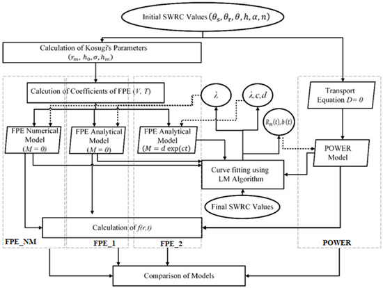
Figure 1.
Methodology flowchart for comparison of different models for predicting PSD evolution.
- (a)
- FPE_1: It represents the analytical solution of FPE found in [24,25]. In this model, was neglected, due to which the first part of the analytical solution, i.e., the exponential term (refer to Equation (12)), was taken as 1. To obtain , the Levenberg–Marquardt (LM) method was used to fit the observed PSD to the one given by Equation (12).
- (b)
- FPE_2: It represents the analytical solution of FPE used by [3,30]. In this, was described as . and were obtained using the LM method, same as that of the FPE_1 model.
- (c)
- NM: It is the numerical model obtained from the finite difference-based discretization of the FPE equation used by [24]. In this model, was neglected.
- (d)
- POWER: It represents the power law model given by [28]. The model coefficients were obtained by curve fitting using the LM method.
3.2. Data
In this study, to compare the performance of four different models to predict the temporal evolution of PSD and SWRC, datasets from various studies across the world have been collected. In addition, the comparison was performed on the SWRC data collected from an experimental agricultural plot at IIT Kanpur, India, for the rice season in 2022. The WP4C Dewpoint Potentiometer from the Meters’ group was used to estimate SWRC from the soil samples taken from the experimental plot. Figure A2 shows a world map showing the various datasets used in the study as well as the experimental site at IIT Kanpur. Table 1 provides the summary of different soil datasets and their classification based on soil type, agriculture practice, land use/cover, and crop type, which have been used in this study for comparison of different models. From the datasets under consideration, the tillage regimes considered are conventional tillage (CT), usually using a moldboard plow, no tillage (NT) with none or very minimal disturbance to the soil, and rototillage (RoT).

Table 1.
Summary of different soil datasets and their classification upon soil type, agriculture practice, cover, crop grown, etc., used in the study.
4. Results and Discussion
The ability of the four different models described earlier to predict PSD evolution, and SWRC was evaluated in this section. The SWRC was obtained for both initial and final conditions using the VG equation for the observed data. The suitability of the models was checked for various agricultural and management practices, such as the crop used, tillage conditions, effects of land-use change and soil type.
Figure 2 shows the prediction of PSD and SWRC evolution over time by different models for chernozem soil in Washington, USA [38]. All the models predicted the PSD evolution very well within the range of observed values. The POWER model over-predicts the PSD values for both the initial (CT) as well as final condition (NT) when μm (see Figure 2a,c). FPE_1, FPE_2 and NM perform well when predicting PSD evolution. However, for predicting SWRC, it was observed that the FPE_1, FPE_2 and NM models underpredict compared to the observed values, while the POWER model is only able to partially predict the values (see Figure 2b,d). The increase in performance of the POWER model can be attributed to higher values of observed .
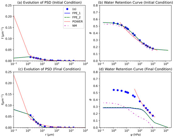
Figure 2.
Comparison of performance of different models of PSD evolution for USA dataset [38]. The soil parameters at initial conditions (CT) are , , and while soil parameters at final conditions (NT) are , , and , respectively.
Figure 3 shows the comparison of performances of different models for predicting the evolution of both soil PSD and SWRC against the observed values for Haplic Cambisol soil from the New Zealand dataset [31]. It was observed that all the models performed well except for the NM model, which underpredicted the soil PSD when (see Figure 3a,c). Similarly, for predicting SWRC, the FPE_1 and FPE_2 models performed well despite FPE_1 slightly underpredicting. Both the NM and POWER models slightly underpredicted and overpredicted the final SWRC values, respectively (see Figure 3b,d).
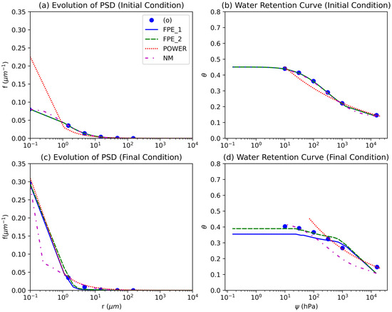
Figure 3.
Comparison of performances of different models of PSD evolution for New Zealand [31]. The soil parameters at initial conditions (CT) are 0.4536, , and while soil parameters at final conditions (pasture) are 0.4093, 0.0830, 2.314 and , respectively.
Figure 4 shows the performances of different models for predicting PSD and SWRC evolution from CT to the plantation for Eutric Fluvisol soil in China [40]. It was observed that NM performed best compared to other models for predicting soil PSD. The FPE_1 and FPE_2 models predicted similar values for both soil PSD as well as SWRC evolution. The PSD values predicted by FPE_1 and FPE_2 was higher as compared to the observed PSD values, while POWER overpredicted soil PSD (see Figure 4c). For predicting SWRC, POWER performed well as compared to others. The FPE_1 and FPE_2 models overpredicted SWRC near saturation and underpredicted it near dryness. NM predicted the least SWRC values for both initial as well as the final condition (see Figure 4a–d).
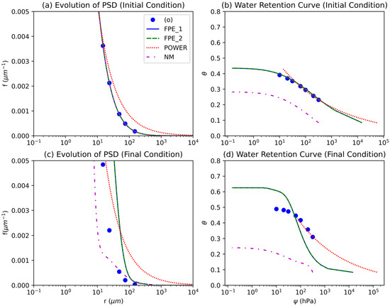
Figure 4.
Comparison of performances of different models of PSD evolution for the China dataset [40]. The soil parameters at initial conditions (CT) are 0.4300, , and while soil parameters at final conditions (forest) are 0.4920, 0.0830, 1.5000 and , respectively.
Figure 5 shows the comparison of different models for predicting PSD and SWRC evolution for Eutric Fluvisol soil from Greece [18]. It was observed that within the observed range of pore radii, all the models accurately predicted PSD as well SWRC (see Figure 5a–d); however, when , the POWER model highly overpredicts soil PSD as compared to other models for both initial as well as final condition. For SWRC, when , POWER overpredicted the values for the initial state, while for the final condition, the model performed well like other models.
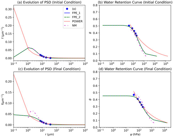
Figure 5.
Comparison of the performances of different models of PSD evolution for the Greece dataset [18]. The soil parameters at initial conditions (RoT, t = 1 day) are 0.521, , and while soil parameters at final conditions (RoT, t = 346 day) are 0.520, 0.065, 1.3421 and respectively.
Figure 6 shows the performance of different models for predicting PSD and SWRC evolution from CT to NT for Hypercalcic Calcisol soil in Spain [41]. The performance of the NM model was best while predicting both soil PSD as well as SWRC evolution. The lowest performance was observed for the POWER model (see Figure 6a–d). FPE_1 and FPE_2 predicted similar values, but they underestimated both soil PSD and SWRC values for the final condition (see Figure 6a–d).
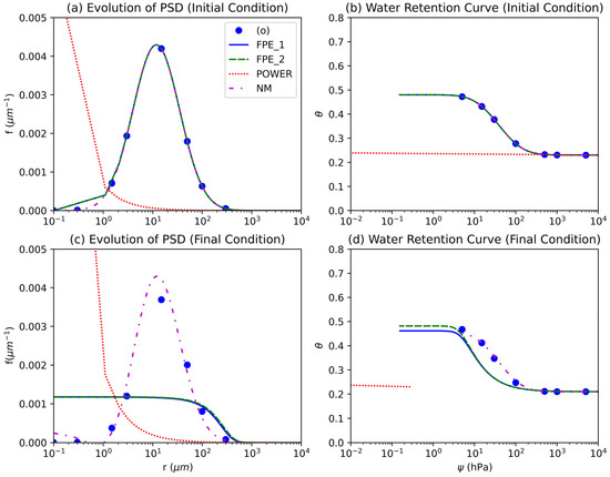
Figure 6.
Comparison of the performances of different models of PSD evolution for the Spain dataset [41]. The soil parameters at initial conditions (CT, t = 1 day) are 0.4800, , and while soil parameters at final conditions (CT, t = 62 day) are 0.4800, 0.21, 1.0807 and respectively.
The performances of different models were compared for predicting PSD and SWRC evolution from CT to NT for Lihen sandy loam soil from the Dakota, USA dataset [42] (Figure 7). It was observed that the FPE_1, FPE_2 and NM models performed well for predicting soil PSD evolution, whereas the POWER overpredicted soil PSD when and underpredicted soil PSD values when for both initial as well as final condition (see Figure 7a,c). For predicting SWRC evolution, the POWER model performed well as compared to the others. FPE_1 and FPE_2 predicted similar results, which were lower than observed SWRC values for both initial as well as final conditions, while NM highly underpredicted SWRC values (see Figure 7b,d).
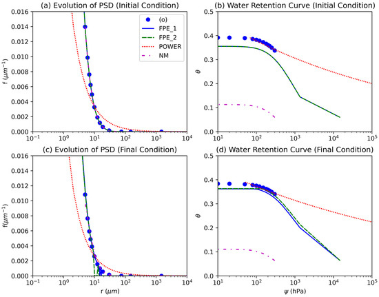
Figure 7.
Comparison of performances of different models of PSD evolution for the USA [42]. The soil parameters at initial conditions (NT, t = 1 day) are 0.3916, , and while the soil parameters at final conditions (NT, t = 365 days) are 0.3836, 0.06370, and respectively.
Figure 8 shows the performance of different models for predicting PSD and SWRC evolution from t = 1 day to t = 30 days under NT conditions for silty loam soil in the experimental agricultural plot at IIT Kanpur, India. Both the FPE_1 and FPE_2 models predicted similar results. However, we were unable to fit the NM and POWER into the observed data. While the performance of the models was poor, they were able to show the temporal evolution of both PSD and SWRC. Modeling of seasonal, temporal variability of SHPs as well as the inclusion of SHPs information for different subplots, may lead to improvement in the performance of the models.
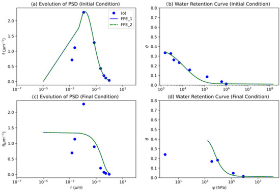
Figure 8.
Comparison of performance of different models of PSD evolution for IIT Kanpur. The soil parameters at initial conditions (NT, t = 1 day) are 0.377, , and while soil parameters at final conditions (NT, t = 30 day) are 0.222, 0.01, and respectively.
The performance of the models was compared for several more datasets, the results of which are not shown for brevity (see Appendix A). Different models for predicting PSD evolution and SWRC were compared for the German dataset of silty loamy soil [34] (see Figure A3). It was observed that the FPE_1 and FPE_2 models well predicted PSD and SWRC evolution. The PSD and SWRC curves by NM and POWER models were found to be underpredicted and overpredicted, respectively. NM predicted PSD and SWRC with higher accuracy when and the model performance decreases when . POWER model underpredicted the initial soil PSD and SWRC at initial conditions when and overpredicted the final PSD and SWRC when .
The four models were compared for datasets from Boreal Forest soils due to compaction by harvesting equipment [35] for the 0th and 3rd skidding cycles (see Figure A4). It was observed that both FPE_1, FPE_2 and POWER models underpredict the final PSD while the final SWRC predicted by FPE_1 and FPE_2 was quite close. The performance of the POWER model was extremely poor for this dataset. The prediction by NM was close to the final soil PSD as well as that of SWRC values (Figure A4b,d).
Figure A5 shows the performance of different models in predicting PSD and SWRC evolution for the 4-year dataset in Chile at depths 0–2 cm and 2–5 cm for sandy clay alluvial soil for initial (CT) and final conditions (NT) [39]. It was observed that the soil PSD as well as SWRC values predicted by FPE_1 and FPE_2 were quite similar and close to the observed values of PSD and SWRC for both depths 0–2 cm and 2–5 cm. FPE_1 and FPE_2 had the best performance among all the models except for predicting SWRC at a depth 0–2 cm, where they overpredicted. For soil PSD prediction, it was observed that the POWER model overpredicts the values for low pore radii for depths 0–2 cm and 2–5 cm. NM overpredicts the values at depths of 0–2 cm, and between 2–5 cm depth, the accuracy of the NM model was improved. However, for predicting SWRC values, it was observed that at the initial condition, the POWER model over and underpredicted at depths 0–2 cm and 2–5 cm, respectively; however, at the final condition, the values predicted by POWER were close to observed values (see Figure A5g,h). For predicting SWRC, NM performed best as compared to others (see Figure A5c,d,g,h). It was observed that with an increase in depth from 0–2 cm to 2–5 cm, the performance of the models improved, and they were able to model soil PSD evolution well.
The PSD and SWRC evolution for the Chile 7-year dataset [39] at depths 0–2 cm and 2–5 cm for sandy clay alluvial soil for initial (CT) and final condition (NT) were best described by the NM (see Figure A6a–e). Both NM and POWER models predicted the final SWRC better as compared to the FPE_1 and FPE_2 models at both 0–2 cm and 2–5 cm depths (see Figure A6g,h). Furthermore, it was observed that, like in the previous case, an improvement in the performance of the FPE_1 and FPE_2 models was observed for the prediction of soil PSD upon an increase in depth from 0–2 cm to 2–5 cm. In addition, the POWER model was found to overpredict the SWRC as well as soil PSD values for the initial condition, but its performance improved for the final condition as well as with an increase in depth.
For the silt loam soil dataset from Austria [14], soil PSD and SWRC evolution were modeled for initial (CT) and final conditions (NT). It was observed that the performances of all the models were satisfactory when lies between the range of observed values (see Figure A7a,b). However, when , the performance of the models varies greatly. The POWER model predicted very large PSD values, while the FPE_1, FPE_2, and NM models predicted lower PSD values in correspondingly decreasing order (see Figure A7a,b). All the models performed well in terms of predicting SWRC. POWER model captured the final SWRC despite overpredicting the initial SWRC. In addition, for the final condition, the SWRC curves from FPE_1 and NM models are higher than that of observed SWRC values, while the FPE_2 model predicted SWRC values close to the observed values (see Figure A7b,d).
Different models were compared in Figure A8 for predicting soil PSD and SWRC evolution against observed values for chernozem soil in the Austria-II dataset [7]. It was observed that all the models performed well while predicting PSD evolution from initial to final state for the observed range of values; however, when predicting SWRC, the performance of the models varies greatly. When , both FPE_2 and POWER models predict high values of the soil PSD while FPE_1 predicts the low PSD values, the predicted PSD values by NM lie in between (see Figure A8b). While predicting SWRC, the POWER and NM models were the most accurate and FPE_2 highly overpredicted, and FPE_1 underpredicted the SWRC values (see Figure A8d). Furthermore, the POWER predicted high values of SWRC as well as soil PSD for the initial condition (see Figure A8a,b), which might be due to its inherent power law assumption.
Different models were compared for Stagnic Luvisol soil with Spring moldboard plowing with maize in France [6]. It was observed that within the observed range of pore radii, POWER and NM models exhibit the best performance in predicting PSD as well SWRC, whereas FPE_1 and FPE_2 models overpredicted (see Figure A9a–d); however, when , it was observed that all the models highly overpredict PSD and SWRC.
4.1. Effect of Tillage
In the above section, it was observed that the performance of different models varies across different sites across the world. In this section, we attempt to discuss how the performance of models varies for similar tillage practices across the world.
For the USA-I (Figure 2), Chile (Figure A4 and Figure A5), Austria-I (Figure A6), Spain (Figure 6) and USA-II (Figure 7), the agricultural practice changes from CT to NT [37,38,40,41]. It was observed that NM performed well in most of the cases while the performance of FPE_1 and FPE_2 was good, but they overpredicted the SWRC values, whereas the POWER performed poorly in most cases except for the Chile dataset, where it was able to predict PSD and SWRC values close to that observed at final conditions despite predicting lower values at initial conditions. Overall, it can be postulated that POWER performed poorly.
The effect of the change of tillage practice from CT to pasture; Moldboard ploughing to NT; CT to the forest were observed in Germany (Figure A3), New Zealand (Figure 3), and China (Figure 4), respectively. It was observed that the FPE_1 and FPE_2 models did not perform as expected; however, the NM and POWER models performed well in those cases.
Overall, it is observed that the FPE_1, FPE_2 and NM Models were able to predict PSD and SWRC evolution for change in tillage as well as the continuation of the same tillage. For better performance of models, higher numbers of observations are required. NM model performed poorly for low pore radii but better as compared to the POWER model.
4.2. Effect of Soil Type
The effect of soil types on models’ performance efficiency was observed for silt loam in Austria-I (Figure A8), Germany (Figure A3) and China (Figure 4) [13,36,40], for sandy clay alluvial soil in Chile (Figure A5 and Figure A6); for Chernozem soil in USA (Figure A2) and Austria-II (Figure A9); Hypercalcic Calcisol soil in New Zealand (Figure 3), for Eutric Fluvisol soil in Greece (Figure 5), respectively. It was observed that for silt loam soil, the values of soil PSD and SWRC for FPE_1 and FPE_2 are quite close to each other as well as close to the observed values except for the China dataset. The POWER and NM models performed well for predicting both PSD and SWRC values.
For sandy clay alluvial soil in Chile, 4- and 7-year datasets from two stations were used to evaluate the models’ performance. It was observed that for silt loam soil, FPE_1 and FPE_2 predicted similar values of PSD and SWRC, which were close to the observed values. NM had the next best performance for both sets of datasets, and while the POWER model underpredicts PSD and SWRC values at the initial state, however, its performance improves for the final condition. Further, it was observed that with an increase in depth, the models’ performance improved (see Figure A5 and Figure A6). For Chernozem soil, it was observed that the FPE_1, FPE_2 and NM models predicted close values of soil PSD but underpredicted SWRC; the POWER model performed best in predicting both PSD and SWRC (see Figure 2 and Figure A9). Furthermore, it was observed that FPE_1 and FPE_2 models predicted different values for both soil PSD and SWRC, unlike previous cases.
It is observed that the performance of the models is highly dependent upon the soil type as it determines the soil PSD as well as available observation data. FPE_1 and FPE_2 predicted similar values and were able to predict the soil PSD and SWRC well for most soil types. NM performed similarly to the FPE_1 and FPE_2 models when predicting both SWRC and PSD. However, the performance of POWER varied highly from the initial condition to the final condition depending upon soil type. POWER performed well if a higher number of observations were present. It was also able to improve its prediction of the final condition despite poor estimation of initial PSD and SWRC values.
5. Conclusions
SHPs exhibit significant spatiotemporal variability and have a strong influence on flow in unsaturated soils. SHPs depend upon the soil structure, which can be described using the soil PSD. The soil PSD and its statistical description as a probability density function are used in the existing predictive models to describe the temporal variation in SHPs. In this study, we compared the performance of four models to describe the temporal evolution of soil PSD and SHPs for various datasets across the world. In addition, the model’s performance was compared to SWRC data collected from an experimental agricultural field at IIT Kanpur. These models were compared for different tillage conditions as well as changes in tillage conditions, soil types, and crop types. Further, an attempt was made to compare the performance of the models for both short-term as well as long-term temporal variability.
Among the four models, two were obtained from the analytical solution of the FPE equation (FPE_1 and FPE_2), and the other two from the POWER and NM models were obtained from the numerical solution of the FPE and power law solution of the generic transport equation. It was observed that when pore radii values were low, the accuracy of the models decreased. The models perform better when the soil pore radii are comparatively high, especially for the POWER and NM models. This correlates to the earlier assumption by [25] that pore-size evolution may affect larger pores as compared to smaller pores. Further, the NM model did not perform well when the number of observed matric potential values were low. The predictive ability of different models was not much affected by changes in tillage condition as that by soil type. The performance of the models was not affected by the crop type. The NM model’s performance can be improved by having more observations, whereas the POWER model is not recommended due to its inherent assumption that soil PSD should follow power law which leads to erroneous values for low soil pore radii. The POWER model performed well when a low number of observations were present, while the FPE_1 and FPE_2 models performed well for most of the cases. For the SWRC dataset obtained from an experimental plot IIT Kanpur, the performance of the POWER and NM models was poor, while the FPE_1 and FPE_2 models performed similarly to each other.
It was observed that models based on the analytical solutions of FPE (FPE_1 and FPE_2) were the best among the models considered, and between them, FPE_1 should be preferred to model the temporal variability of SHPs and PSD. Furthermore, to improve the performance of models, more observations are required for modeling both short and long-term temporal variation in SHPs. Future studies should focus not only on modeling the temporal variability of SHPs but also on relating the parameters of FPE with the various agricultural practices in the field, which can be useful for effective water management.
Author Contributions
Conceptualization, S.K. and R.O.; methodology, investigation, validation, formal analysis, S.K.; writing—original draft preparation, S.K.; writing—review and editing, supervision, R.O. All authors have read and agreed to the published version of the manuscript.
Funding
The authors would like to thank the financial support from the Science and Engineering Research Board, Government of India, for the project titled “Temporal Variability of Soil Hydraulic Properties in Agricultural Field” through project no. CRG/2021/003340.
Institutional Review Board Statement
Not applicable.
Informed Consent Statement
Not applicable.
Data Availability Statement
The data presented in this study are publicly available.
Conflicts of Interest
The authors declare conflict of interest with Chandra Shekhar Prasad Ojha. We request to remove his name from the academic editor(s) list as he was not the handling editor for this paper.
Appendix A

Figure A1.
Comparison of analytical and numerical solution of FPE with time-dependent term V(t), where λ = 1, 0.469, 0.191, 0.253, 7.3 , 7.5, , and . Analytical refers to analytical solution models used by both [2,22,23], and numerical refers to the numerical solution of FPE.

Figure A2.
(a) Various datasets used in this study across the world; and (b) experimental agricultural plot at IIT Kanpur.

Figure A3.
Comparison of performances of different models of PSD evolution for Germany dataset [33]. The soil parameters at initial conditions (Moldboard Plowing) are , , and while soil parameters at final conditions (NT) are 0.392, , and respectively.

Figure A4.
Comparison of performance of different models of PSD evolution for test of compaction between empty and loaded pass in West-central Alberta [34]. The soil parameters at initial conditions (0th skidding cycle) are 0.55, , and while soil parameters at final conditions (3rd skidding cycle) are , , and respectively.

Figure A5.
Comparison of performances of different models of PSD evolution for the Chile 4-year dataset at depths 0–2 cm and 2–5 cm [36]. For depth 0–2 cm, the soil parameters at initial conditions (CT) are , , while soil parameters at final conditions (NT) are 0.4288, , and respectively, while for depth 2–5 cm, the soil parameters at initial conditions (CT) are 0.4971, , and while soil parameters at final conditions (NT) are 0.4555, , and respectively.

Figure A6.
Comparison of performances of different models of PSD evolution for the Chile 7-year dataset at 0–2 cm depths [36]. For depth 0–2 cm, the soil parameters at initial conditions (CT) are , , and while soil parameters at final conditions (NT) are 0.4571, , and respectively, while for depth 2–5 cm, the soil parameters at initial conditions (CT) are 0.4971, , and while soil parameters at final conditions (NT) are 0.4555, , and , respectively.

Figure A7.
Comparison of performance of different models for PSD evolution for Austria I dataset [11]. The soil parameters at initial conditions (CT) are , , and while soil parameters at final conditions (NT) are , , and respectively.

Figure A8.
Comparison of performances of different models for PSD evolution for Austria II dataset [6]. The soil parameters at initial conditions (CT; t = 1 day) are , , and while soil parameters at final conditions (CT; t = 181 day) are , , and respectively.

Figure A9.
Comparison of performances of different models of PSD evolution for the France dataset [4]. The soil parameters at initial conditions (NT, t = 1 day) are 0.342, , and while soil parameters at final conditions (NT, t = 147 day) are 0.322, 0, and respectively.
References
- Bonfante, A.; Sellami, M.H.; Abi Saab, M.T.; Albrizio, R.; Basile, A.; Fahed, S.; Giorio, P.; Langella, G.; Monaco, E.; Bouma, J. The role of soils in the analysis of potential agricultural production: A case study in Lebanon. Agric. Syst. 2017, 156, 67–75. [Google Scholar] [CrossRef]
- Chandrasekhar, P.; Kreiselmeier, J.; Schwen, A.; Weninger, T.; Julich, S.; Feger, K.H.; Schwärzel, K. Why we should include soil structural dynamics of agricultural soils in hydrological models. Water 2018, 10, 1862. [Google Scholar] [CrossRef]
- Chandrasekhar, P.; Kreiselmeier, J.; Schwen, A.; Weninger, T.; Julich, S.; Feger, K.H.; Schwärzel, K. Modeling the evolution of soil structural pore space in agricultural soils following tillage. Geoderma 2019, 353, 401–414. [Google Scholar] [CrossRef]
- Corey, A.T. Measurement of water and air permeability in unsaturated soil. Soil Sci. Soc. Am. J. 1957, 21, 7–10. [Google Scholar] [CrossRef]
- Jirků, V.; Kodešová, R.; Nikodem, A.; Mühlhanselová, M.; Žigová, A. Temporal variability of structure and hydraulic properties of topsoil of three soil types. Geoderma 2013, 204, 43–58. [Google Scholar] [CrossRef]
- Alletto, L.; Pot, V.; Giuliano, S.; Costes, M.; Perdrieux, F.; Justes, E. Temporal variation in soil physical properties improves the water dynamics modeling in a conventionally-tilled soil. Geoderma 2015, 243, 18–28. [Google Scholar] [CrossRef]
- Bodner, G.; Scholl, P.; Kaul, H.P. Field quantification of wetting–drying cycles to predict temporal changes of soil pore size distribution. Soil Tillage Res. 2013, 133, 1–9. [Google Scholar] [CrossRef]
- Zhang, M.; Lu, Y.; Heitman, J.; Horton, R.; Ren, T. Temporal changes of soil water retention behavior as affected by wetting and drying following tillage. Soil Sci. Soc. Am. J. 2017, 81, 1288–1295. [Google Scholar] [CrossRef]
- Blackman, J.D. Seasonal variation in the aggregate stability of downland soils. Soil Use Manag. 1992, 8, 142–150. [Google Scholar] [CrossRef]
- Moreira, W.H.; Tormena, C.A.; Karlen, D.L.; da Silva, Á.P.; Keller, T.; Betioli, E., Jr. Seasonal changes in soil physical properties under long-term no-tillage. Soil Tillage Res. 2016, 160, 53–64. [Google Scholar] [CrossRef]
- Bodner, G.; Loiskandl, W.; Buchan, G.; Kaul, H.P. Natural and management-induced dynamics of hydraulic conductivity along a cover-cropped field slope. Geoderma 2008, 146, 317–325. [Google Scholar] [CrossRef]
- Alletto, L.; Coquet, Y. Temporal and spatial variability of soil bulk density and near-saturated hydraulic conductivity under two contrasted tillage management systems. Geoderma 2009, 152, 85–94. [Google Scholar] [CrossRef]
- Schwen, A.; Bodner, G.; Loiskandl, W. Time-variable soil hydraulic properties in near-surface soil water simulations for different tillage methods. Agric. Water Manag. 2011, 99, 42–50. [Google Scholar] [CrossRef]
- Schwen, A.; Bodner, G.; Scholl, P.; Buchan, G.D.; Loiskandl, W. Temporal dynamics of soil hydraulic properties and the water-conducting porosity under different tillage. Soil Tillage Res. 2011, 113, 89–98. [Google Scholar] [CrossRef]
- Kargas, G.; Kerkides, P.; Sotirakoglou, K.; Poulovassilis, A. Temporal variability of surface soil hydraulic properties under various tillage systems. Soil Tillage Res. 2016, 158, 22–31. [Google Scholar] [CrossRef]
- Kreiselmeier, J.; Chandrasekhar, P.; Weninger, T.; Schwen, A.; Julich, S.; Feger, K.H.; Schwärzel, K. Quantification of soil pore dynamics during a winter wheat cropping cycle under different tillage regimes. Soil Tillage Res. 2019, 192, 222–232. [Google Scholar] [CrossRef]
- Kreiselmeier, J.; Chandrasekhar, P.; Weninger, T.; Schwen, A.; Julich, S.; Feger, K.H.; Schwärzel, K. Temporal variations of the hydraulic conductivity characteristic under conventional and conservation tillage. Geoderma 2020, 362, 114127. [Google Scholar] [CrossRef]
- Geris, J.; Verrot, L.; Gao, L.; Peng, X.; Oyesiku-Blakemore, J.; Smith, J.U.; Hodson, M.E.; McKenzie, B.M.; Zhang, G.; Hallett, P.D. Importance of short-term temporal variability in soil physical properties for soil water modelling under different tillage practices. Soil Tillage Res. 2021, 213, 105132. [Google Scholar] [CrossRef]
- Xu, D.; Mermoud, A. Modeling the soil water balance based on time-dependent hydraulic conductivity under different tillage practices. Agric. Water Manag. 2003, 63, 139–151. [Google Scholar] [CrossRef]
- Feki, M.; Ravazzani, G.; Ceppi, A.; Mancini, M. Influence of soil hydraulic variability on soil moisture simulations and irrigation scheduling in a maize field. Agric. Water Manag. 2018, 202, 183–194. [Google Scholar] [CrossRef]
- Šípek, V.; Jačka, L.; Seyedsadr, S.; Trakal, L. Manifestation of spatial and temporal variability of soil hydraulic properties in the uncultivated Fluvisol and performance of hydrological model. Catena 2019, 182, 104119. [Google Scholar] [CrossRef]
- Zhao, W.; Cui, Z.; Zhou, C. Spatiotemporal variability of soil–water content at different depths in fields mulched with gravel for different planting years. J. Hydrol. 2020, 590, 125253. [Google Scholar] [CrossRef]
- Villarreal, R.; Lozano, L.A.; Salazar, M.P.; Bellora, G.L.; Melani, E.M.; Polich, N.; Soracco, C.G. Pore system configuration and hydraulic properties. Temporal variation during the crop cycle in different soil types of Argentinean Pampas Region. Soil Tillage Res. 2020, 198, 104528. [Google Scholar] [CrossRef]
- Or, D.; Leij, F.J.; Snyder, V.; Ghezzehei, T.A. Stochastic model for posttillage soil pore space evolution. Water Resour. Res. 2000, 36, 1641–1652. [Google Scholar] [CrossRef]
- Leij, F.J.; Ghezzehei, T.A.; Or, D. Analytical models for soil pore-size distribution after tillage. Soil Sci. Soc. Am. J. 2002, 66, 1104–1114. [Google Scholar] [CrossRef]
- Leij, F.J.; Ghezzehei, T.A.; Or, D. Modeling the dynamics of the soil pore-size distribution. Soil Tillage Res. 2002, 64, 61–78. [Google Scholar] [CrossRef]
- Maggi, F.; Porporato, A. Coupled moisture and microbial dynamics in unsaturated soils. Water Resour. Res. 2007, 43. [Google Scholar] [CrossRef]
- Pelak, N.; Porporato, A. Dynamic evolution of the soil pore size distribution and its connection to soil management and biogeochemical processes. Adv. Water Resour. 2019, 131, 103384. [Google Scholar] [CrossRef]
- Brooks, R.H. Hydraulic Properties of Porous Media; Colorado State University: Fort Collins, CO, USA, 1965. [Google Scholar]
- Clapp, R.B.; Hornberger, G.M. Empirical equations for some soil hydraulic properties. Water Resour. Res. 1974, 14, 601–604. [Google Scholar] [CrossRef]
- Schwärzel, K.; Carrick, S.; Wahren, A.; Feger, K.H.; Bodner, G.; Buchan, G. Soil hydraulic properties of recently tilled soil under cropping rotation compared with two-year pasture. Vadose Zone J. 2011, 10, 354–366. [Google Scholar] [CrossRef]
- Hara, T. A stochastic model and the moment dynamics of the growth and size distribution in plant populations. J. Theor. Biol. 1984, 109, 173–190. [Google Scholar] [CrossRef]
- Bodner, G.; Leitner, D.; Kaul, H.P. Coarse and fine root plants affect pore size distributions differently. Plant Soil 2014, 380, 133–151. [Google Scholar] [CrossRef] [PubMed]
- Kosugi, K.I. Lognormal distribution model for unsaturated soil hydraulic properties. Water Resour. Res. 1996, 32, 2697–2703. [Google Scholar] [CrossRef]
- Van Genuchten, M.T. A closed-form equation for predicting the hydraulic conductivity of unsaturated soils. Soil Sci. Soc. Am. J. 1980, 44, 892–898. [Google Scholar] [CrossRef]
- Teiwes, K. Einfluß von Bodenbearbeitung und Fahrverkehr auf physikalische Eigenschaften schluffreicher Ackerböden. Ph.D. Thesis, University of Göttingen, Göttingen, Germany, 1988. [Google Scholar]
- Startsev, A.D.; McNabb, D.H. Skidder traffic effects on water retention, pore-size distribution, and van Genuchten parameters of boreal forest soils. Soil Sci. Soc. Am. J. 2001, 65, 224–231. [Google Scholar] [CrossRef]
- Fuentes, J.P.; Flury, M.; Bezdicek, D.F. Hydraulic properties in a silt loam soil under natural prairie, conventional till, and no-till. Soil Sci. Soc. Am. J. 2004, 68, 1679–1688. [Google Scholar] [CrossRef]
- Martínez, E.; Fuentes, J.P.; Silva, P.; Valle, S.; Acevedo, E. Soil physical properties and wheat root growth as affected by no-tillage and conventional tillage systems in a Mediterranean environment of Chile. Soil Tillage Res. 2008, 99, 232–244. [Google Scholar] [CrossRef]
- Yu, M.; Zhang, L.; Xu, X.; Feger, K.H.; Wang, Y.; Liu, W.; Schwärzel, K. Impact of land-use changes on soil hydraulic properties of Calcaric Regosols on the Loess Plateau, NW China. J. Plant Nutr. Soil Sci. 2015, 178, 486–498. [Google Scholar] [CrossRef]
- Peña-Sancho, C.; López, M.V.; Gracia, R.; Moret-Fernández, D. Effects of tillage on the soil water retention curve during a fallow period of a semiarid dryland. Soil Res. 2016, 55, 114–123. [Google Scholar] [CrossRef]
- Jabro, J.D.; Stevens, W.B. Soil-water characteristic curves and their estimated hydraulic parameters in no-tilled and conventionally tilled soils. Soil Tillage Res. 2022, 219, 105342. [Google Scholar] [CrossRef]
Disclaimer/Publisher’s Note: The statements, opinions and data contained in all publications are solely those of the individual author(s) and contributor(s) and not of MDPI and/or the editor(s). MDPI and/or the editor(s) disclaim responsibility for any injury to people or property resulting from any ideas, methods, instructions or products referred to in the content. |
© 2023 by the authors. Licensee MDPI, Basel, Switzerland. This article is an open access article distributed under the terms and conditions of the Creative Commons Attribution (CC BY) license (https://creativecommons.org/licenses/by/4.0/).