Article

Analysis of the Impact of Carbon Emission Control on Urban Economic Indicators based on the Concept of Green Economy under Sustainable Development

1
School of Economics, Faculty of Economics, Liaoning University, Shenyang 110036, China
2
Graduate School, Chinese Academy of Fiscal Sciences, Beijing 100142, China
3
Nanyang Centre for Public Administration (NCPA), Nanyang Technological University (NTU), Singapore 637598, Singapore
*
Author to whom correspondence should be addressed.
Sustainability 2023, 15(13), 10145; https://doi.org/10.3390/su151310145
Submission received: 15 May 2023 / Revised: 16 June 2023 / Accepted: 20 June 2023 / Published: 26 June 2023
(This article belongs to the Section Economic and Business Aspects of Sustainability)

Abstract

:
With the deepening of the concept of sustainable development, a green economy has become the primary goal of urban development. Therefore, to improve the sustainability and far-reaching development of the urban economy, this work first discusses the concept of sustainable development. Second, the concept of a “green economy” is discussed. Lastly, based on the concept of green economic development, this work studies carbon emissions in Hebei Province, China, and discusses the impact of carbon emissions on the urban economy. On this basis, the impact of carbon intensity and CO2 emissions on economic growth is analyzed by establishing an endogenous growth model and state-space model, thereby revealing the importance of carbon emissions to the economic development of Hebei Province. In the analysis process, sensitivity analysis and a robustness test are also used to verify the reliability and robustness of the model results. Finally, this work summarizes the research conclusions and puts forward relevant policy suggestions, which provide a reference for developing a green economy in Hebei Province. The results reveal that from 1999 to 2020, the average output elasticity of labor, capital, and CO2 in Hebei Province are 0.4002, 0.3057, and 0.2941, respectively. This shows that carbon emissions are essential to Hebei’s economic growth. In other words, Hebei’s economic development mainly depends on enterprises with high carbon emissions. Additionally, in the optimistic case, Hebei’s potential output growth rate will show a downward trend, but will soon rise. This indicates that even under strict carbon emission control, Hebei’s economic growth rate will still pick up based on the support of high-tech. This work not only provides a reference for the development of Hebei’s green economic system, but also contributes to the sustainable development of the urban economy in the future.

1. Introduction

Today, the severe environmental impact of global warming has surfaced, which has aroused widespread concern worldwide. Relevant research shows that CO2 generated by fossil combustion is the main cause of global warming despite fossil energy playing a crucial role in China’s economic development [1]. Therefore, how to control carbon emissions while maintaining economic growth is the key issue in China [2]. The Netherlands Environmental Assessment Bureau reported in 2007 that “China has become the country with the largest CO2 emissions, and it is urgent to build a green and environment-friendly economic system”. Consequently, to protect the environment and promote the continuous progress of human society, the concept of a green economy came into being. With the continuous improvement of the economic system, building a green economic system has become a feasible social development measure. In fact, protecting the environment and improving the economic growth model have become necessary conditions for economic development. As a large energy production and consumption province, Hebei Province also has relatively high CO2 emissions. In recent years, with the acceleration of industrialization, this province’s environmental pollution has been severe [3]. Hebei Province is still mainly dependent on coal and has a relatively undiversified energy structure. Developing tertiary industry and green new energy is a big challenge in Hebei Province. At present, the whole society pays more and more attention to developing a green economy, so it is imperative to study the green economy and its sustainable development concept. Based on this, many studies have provided references for developing the green economy.
Ali et al. (2021) comprehensively evaluated global studies on the green economy and sustainable development through bibliometric analysis. The results showed that research on the green economy and sustainable development presented a trend of steady growth, while there were differences between countries and the differentiation of disciplines [4]. Yang et al. (2022) discussed the development status and future trends of sustainable development and the green economy in China. By analyzing policies, industries, finance, and other aspects, the study concluded that China had made remarkable progress in promoting sustainable development and a green economy. However, it still needed to strengthen policy coordination, technological innovation, market orientation, and other aspects [5]. Falcone et al. (2021) took emerging economies as research objects and analyzed the status quo of their sustainable development and green economy. They explored emerging economies’ challenges and opportunities in promoting sustainable development and a green economy. The study argued that emerging economies had great potential and advantages in sustainable development and green economy, but they still needed to strengthen policy support, technological innovation, and international cooperation [6]. Karintseva et al. (2021) selected the European Union (EU) as the research object and analyzed the status quo of its sustainable development and green economy. The achievements and experiences of the EU in promoting sustainable development and a green economy were discussed. The study concluded that the EU had formed a series of policies and action plans for sustainable development and a green economy and had achieved remarkable results. At the same time, they also put forward the areas and measures that the EU should further strengthen in promoting sustainable development and a green economy in the future [7]. Sustainable development and the green economy were comprehensive issues involving multiple disciplines and fields, which required interdisciplinary and cross-field research to comprehensively and deeply explore their various aspects. The relevant studies were often limited to a specific area or discipline, lacking in comprehensiveness, and unsystematic.
Therefore, in the context of current sustainable development, this work studies the impact of carbon emission control on economic growth under a green economy to improve the economic development level of Hebei Province. The proposed scheme plays a vital role in the sustainable economic development of Hebei Province and provides a reference for the establishment of the national green economy model. The national and provincial governments have set specific policies for Hebei to control carbon emissions, but total emissions still stubbornly remain high. The proportion of coal in the local energy structure is still very high, and problems remain prominent. Therefore, taking Hebei Province as an example, this work uses quantitative analysis and empirical analysis to specifically analyze the economic growth rate of Hebei Province under the control of carbon emissions. Firstly, the relevant theoretical content is discussed. Secondly, a research method based on carbon emission control is designed. Finally, the research results are provided through data analysis, and corresponding suggestions for future development are provided.

2. Theory and Model Analysis

2.1. Related Theoretical Basis Analysis

2.1.1. Sustainable Development Theory

Suparjo et al. (2021) noted that Indonesia was participating in global change to achieve this mission by accelerating the development programs included in the sustainable development goals. Green growth was part of achieving sustainable development and was determined by the empowerment of Indonesia’s energy sector, such as light sources, the renewable energy mix, and primary energy intensity. They used the ordinary least square method model to analyze the time series data. The significance of this study was to draw attention to these findings and make essential points for the sustainable development goal document for the energy sector. This also indicated that Indonesia needed to pay more attention to realizing green growth in promoting sustainable development, focusing on factors such as the renewable energy mix, light sources, and primary energy intensity. At the same time, this study also provided reference and inspiration for other countries and regions in achieving sustainable development [8]. It can be found that the development of the green economy is constantly optimized, which will undoubtedly have a substantial impact on the overall development of society in the future.
The green economy and sustainable development are interrelated, emphasizing harmonious development between human beings and nature. The green economy refers to the sustainable development of the economy, society, and environment by reducing environmental pollution and resource consumption while improving productivity and increasing employment [9]. Sustainable development means meeting current needs without harming the needs of future generations and achieving a balanced development of the economy, society, and environment. A green economy positively impacts sustainable development and can achieve coordinated economic, social, and environmental development. The following are some critical impacts of the green economy on sustainable development:
(1) Resource efficiency and circular economy: The green economy emphasizes the effective use and recycling of resources, and achieves the sustainable use of resources by improving the production process and product design, reducing resource consumption and waste generation. This helps to reduce pressure on the environment, reduce dependence on natural resources and promote long-term sustainable economic development.
(2) Innovation and technological development: The green economy promotes the development of clean technology and sustainable innovation, providing new growth drivers for economic growth. Investing in green technologies and industries can promote the transformation and upgrading of economic structure, thus improving sustainable economic development.
(3) Employment and social inclusion: The green economy creates a large number of jobs, especially in the fields of renewable energy, environmental protection, and energy efficiency. This is conducive to increasing employment and social inclusion, reducing poverty and social inequality, and achieving sustainable economic and social development.
(4) Ecosystem protection and biodiversity: The green economy focuses on the importance of ecosystem protection and biodiversity. Ecosystem health and sustainable development can be ensured by protecting the natural environment and ecosystem functions and maintaining biodiversity. This is essential for human survival and long-term economic growth.
In a word, the green economy is closely related to sustainable development. Through resource efficiency, the circular economy, innovation, employment, social inclusion, ecosystem protection, and other aspects, the coordinated development of the economy, society, and environment is promoted, and the goal of sustainable development is achieved.
Nowadays, sustainable development is involved in many fields. The definitions differ vastly. One theory, which the international community has widely recognized, states that sustainable development can meet contemporary people’s needs while not harming future generations’ needs. Its basic principles are fairness, sustainability, and commonality [10].
Since 1950, environmental quality has seen a great decline. In this context, the traditional economic model is questioned with the deteriorating ecological environment, even though it has contributed to rapid economic development. Therefore, a UN (United Nations) report proposed the concept of sustainable development in the second half of the 20th century to promote environmental-friendly natural resource utilization [11,12,13,14].

2.1.2. Kuznets Curve

The Kuznets Curve is a theory put forward by the economist Kuznets in the middle of the 20th century. The theory initially describes the relationship between the degree of distribution fairness and economic growth, and it contends that there is an inverted U-shaped relationship between income distribution fairness and economic growth [15]. Later, scholars point out an inverted U-shape relationship between economy and environmental quality, where the Kuznets Curve can be used for analysis, thus the EKC (Environmental Kuznets Curve). So far, the results of the EKC are developed into six categories, as plotted in Figure 1.

2.2. Model-Building

2.2.1. Accounting Equation of Potential Growth

Crafts and Woltjer (2021) used accounting equations to analyze the relationship between South Africa’s potential growth rate and fiscal consolidation. Studies indicated that fiscal consolidation could promote potential growth by increasing private investment and participation in the labor force [16]. Vospernik (2021) explored the impact of accounting equations on Indonesia’s economic growth and focused on the role of investment and government spending in economic growth. It was found that investment and government expenditure significantly positively impacted Indonesia’s economic growth [17]. Thus, through the application of accounting equations, the researchers revealed the importance of fiscal integration, investment, and government expenditure to economic growth. The promotion effect of fiscal consolidation on economic growth was mainly reflected in stimulating private investment and improving the labor force participation rate. Meanwhile, the positive impact of investment and government expenditure on economic growth indicated that increasing investment and strengthening government expenditure was of great significance in promoting economic growth. These findings provided useful references for policymakers, especially in the areas of fiscal consolidation, investment, and government expenditure. By strengthening fiscal consolidation measures and raising private investment and labor force participation, the release of economic potential can be further promoted, and sustainable development can be achieved. Moreover, increasing support for investment and government expenditures can provide a stable driving force for economic growth and promote the sustainable development of society as a whole.
Cobb–Douglas is a production function that describes the relationship between input and output, which is extensively used in economics. The specific calculation reads:
Y t = A K t α L t β
Equation (1) is the traditional Cobb–Douglas production function, without considering the impact of carbon emissions on the economy, where A—Total factor productivity, K—Actual output in a certain period, L—Labor input in a certain period, and α , β —Output elasticity of capital and labor and are fixed constants. Remarkably, the environment and economic structure of Hebei Province are facing severe threats. Under such environmental conditions, α , β are not fixed constants. Therefore, based on previous studies, this work re-adjusts the production function, as shown in Equation (2).
Y t = A ( t ) K t α k L t α l C t α c = A 0 e α A t K t α k L t α l C t α c
In Equation (2), C—Carbon emissions in a certain period, α k , α l , α c —Output elasticity of time-varying capital, labor, and CO2.
The calculation of total factor productivity is:
A ( t ) = A 0 e α A t
In Equation (3), A0—Initial technical level, and α A —Technological growth.

2.2.2. State-Space Model

Generally, time series and regression analyses can be used to estimate unknown parameters for observable variables. However, in real economic systems, not all states are observable, represented by the state vector [18,19]. Here, the unobservable variables include the output elasticity of labor, capital, and CO2 and the growth rate of total factor productivity, all of which belong to the state vector [20]. The state-space model effectively estimates the model with unobservable variables and can reflect the relationship between observable variables and state vectors. Therefore, the state-space model is used to estimate the production function here.
If the return-to-scale does not change, namely, α k + α l + α c = 1 , then Equation (4) can be obtained by taking logarithms on both sides.
ln Y t = ln A 0 + α A t × t + α k t × ln K t + ( 1 α k t α c t ) × ln L t + α c t × ln C t
If ln A 0 = b, the state-space model can be implemented as follows.
Measurement equation:
ln Y t = b + r t × t + α t × ln K t + ( 1 α k t α c t ) × ln L t + α c t × ln C t + μ b
State equations:
α k t = π + λ × α k t 1 + μ t
α c t = α c t 1 + ζ t
α A t = α A t 1 + η t
where ln Y t , ln K t , ln L t , ln C t —Observable variable, α k t , α c t , α A t —Unobservable state vector that needs to be estimated.
The above research methods play an important role in studying the influence of carbon emission control on economic growth in a green economy. The traditional Cobb–Douglas production function does not consider the impact of carbon emissions on economic growth. Hence, the production function needs to be recalibrated to assess the effects of carbon emissions on economic growth more accurately. At the same time, the state-space model can be used to estimate unobserved variables to more accurately evaluate the influence of carbon emissions on economic growth.
Using the above research methods, the impact of carbon emission control on economic growth under the green economy can be more accurately evaluated, providing valuable references and suggestions for policymakers. Based on the research results, policymakers can better understand the relationship between environmental protection and economic growth and formulate corresponding policy measures to promote a win-win situation of economic growth and environmental protection. In addition, the research method also offers a practical method of exploration for academic research in related fields and provides theoretical support for further promoting a green economy and sustainable development. Therefore, the above research methods play a vital and significant in studying the impact of carbon emission control on economic growth under the green economy.

2.3. Index Selection and Data Description

2.3.1. Estimation of Capital Stock

Since there are no ready-made data for reference, the capital stock is measured by the widely used perpetual stock method [21]. The specific algorithm reads:
K t = I t / P t + ( 1 δ t ) K t 1
In Equation (9), K—Actual capital stock of a certain year (priced at the constant price of the base year), I—Investment amount of fixed assets in a certain year (expressed at current price), P—Fixed asset investment price index based on a certain year, and δ t —Depreciation rate of a certain year [22,23,24].
Determination of Pt (Fixed asset investment price index): The data were obtained from previous research results. However, the Hebei Economic Yearbook only gives the Pt value of Hebei Province from 1990 to 2016. Comparative analysis shows little difference between the Pt value of Hebei Province and the national Pt value in China. Therefore, this work uses the national Pt value from 1978 to 1989 to replace the Pt value of Hebei Province in the corresponding year [25].
Determination of It (Fixed asset investment): the data come from the Hebei Economic Yearbook [26].
The Determination of δ t (Depreciation rate of fixed assets): based on the research of Wang Xiaolu and Meng Lian (2000), δ t is assumed to be 5%.
The K value from 1999 to 2020 is calculated through Equation (8) as the basic data.

2.3.2. Y (Actual Output)

Y is a translation calculation of the GDP data of Hebei Province from 1978 to 2016 through the regional GDP index (the regional GDP index was set to 100 in 1978), namely, the data for 1999–2020 are obtained [27]. The above data are all from the Hebei Economic Yearbook. The data from 1999 to 2020 were chosen because this period was one of the most rapid periods of economic growth since China’s reform and opening-up. It was also a critical period for economic growth in Hebei Province. China implemented economic reforms and policy measures during this period, significantly promoting rapid economic growth. At the same time, Hebei Province, a substantial manufacturing base and transportation hub in China, also developed rapidly during this period. Hence, the data from this period can better reflect the overall trend and characteristics of economic growth in Hebei Province and provide more accurate and comprehensive data support for the study of economic growth in Hebei. Furthermore, the data of this period also have high comparability and stability, which is conducive to horizontal and vertical comparative analysis.

2.3.3. L (Labor)

The number of employed persons in Hebei Province from 1999 to 2020 is downloaded from the official website of the National Bureau of Statistics (NBS) [28,29].

2.3.4. CO2 Emissions

China has not published data on CO2 emissions, so the energy consumption method is used to estimate CO2 emissions. The specific algorithm reads:
C O 2 = i = 1 8 C O 2 , i = i = 1 8 E i × C C O 2 , i
C O 2 , i —CO2 emitted by the above 8 kinds of energy consumption, Ei—overall energy consumption of eight kinds of energy consumption, and CCO2,i—CO2 emission factor of eight kinds of energy consumption.

2.4. Impact of Low Carbon Transformation on Economic Growth under the Endogenous Growth Model

This work systematically analyzes the relationship between carbon emission control and the economy based on endogenous CO2 emission control [30,31]. The model implementation can be written as Equations (11) and (12):
max 0 e ρ t ( C t 1 ξ 1 1 ξ S 1 + θ + 1 1 + θ ) d t
s . t . { Y t = z t ψ A 1 1 γ K t α 1 γ [ D T ( 1 n t ) ] β 1 γ ( G t π μ t ) γ 1 γ K t = Y t C t D t = η n t D t E = ω ( 1 μ t ) E t G t Y t π S = G t Y t d S t } ,   α + β + γ = 1 , ψ > γ 1 γ > 0
The six equations in the proposed model represent the social welfare function, the production function including CO2 emission factors, the motion equation of capital accumulation, technology level, energy input, and the equation of CO2 emissions accumulated in the atmosphere [32,33,34]. To sum up, this work conducts a comprehensive evaluation of the economic development of Hebei Province according to the proposed model. The data are from the official website of the NBS and the official website of the Hebei Provincial Bureau of Statistics.

3. Calculation of Potential Output and Economic Growth Rate of Hebei Province under Carbon Emission Control

3.1. Model Solution of the Impact of Carbon Emission Control on Economic Growth

3.1.1. Calculation Results of the Endogenous Growth Model

The endogenous growth model is used in economics to explain long-term economic growth. It emphasizes the importance of technological progress and human capital accumulation for economic growth. When calculating the endogenous growth model, it is necessary to determine some parameters, such as savings rate, marginal output rate of capital, etc., and some initial values, such as capital stock and population. By setting these parameters and initial values, the calculation results of the model, such as economic growth rate and capital accumulation rate, can be obtained. Therefore, when calculating the endogenous growth model, this work ensures that the set of parameters and initial values is scientific and reasonable through scientific research methods and norms. At the same time, the model‘s sensitivity analysis and robustness test are carried out to verify the reliability and robustness of the calculated results. Furthermore, this method corresponds to the previous section’s method to jointly test and analyze the massive development data of Hebei Province. It not only realizes technological innovation but also better improves the accuracy of research data calculation, to highlight the value of this work.
According to the optimal calculation of economic growth, the Hamilton model is implemented, as follows:
H = U ( C t , S t ) + λ 1 ( Y t C t ) + λ 2 η n t D t + λ 3 [ ϖ ( 1 μ t ) E t G t Y t π ] + λ 4 ( G t Y t d S t )
where C , n , z , G —Control variable, K , D , E , S —Condition variables, λ 1 —Capital stock, λ 2 —Technology accumulation, λ 3 —Energy consumption, and λ 4 —CO2 accumulation.
The variable is set to x, g x is used to express its growth rate, and g x is a constant value. Then, the results of the proposed model read:
g Y = { β 1 γ η n ψ [ ρ ω ( 1 μ ) ] ( ψ γ 1 γ ) g G } ( β 1 γ + ψ ξ ) 1
g Y = { β 1 γ η n γ 1 γ [ ρ ω ( 1 μ ) ] φ 1 φ ( ψ γ 1 γ ) g φ } ( β + γ ξ 1 γ ) 1
g s = 1 θ [ ρ ω ( 1 μ ) φ ( ψ γ 1 γ ) φ ( ψ γ 1 γ ) + γ 1 γ g φ ]
Equations (14) and (15) show that only when g Y is positive can the economy maintain a growing trend. At this time, g G , g φ must meet the following requirements:
g G < g G = { β 1 γ η n ψ [ ρ ω ( 1 μ ) ] } ( ψ γ 1 γ )
g φ < g φ = ( 1 φ 1 ) { β 1 γ η n γ 1 γ [ ρ ω ( 1 μ ) ] } ( ψ γ 1 γ ) 1
According to Equation (16), the main influencing factor of cumulative carbon emission in the atmosphere is g φ , and g s is negative only when Equation (19) holds.
g φ > g φ = [ ρ ω ( 1 μ ) ] [ 1 + γ 1 γ φ ( ψ γ 1 γ ) ]

3.1.2. Determination of Capital Stock and CO2 in the Base Period

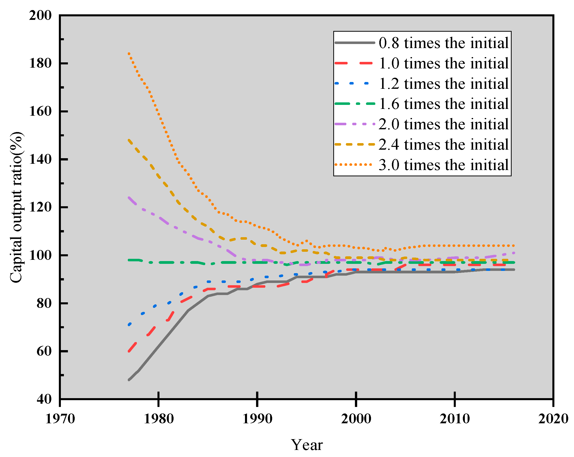
The base year chosen in this work is 1978. In the available literature, China’s stock in 1978 is estimated to be about 0.9–3 times actual output. Specifically, referring to the method adopted by Wu Guobao in 2015, the ratio of capital stock to actual output is set as 0.8, 1, 1.2, 1.6, 2, 2.4, and 3, respectively, and the capital stock is estimated under different ratios. All the data charts below are from the processing results of the GDP data of Hebei Province from 1999 to 2020. The results are displayed in Figure 2.
Figure 2 signifies that when other things are equal, the gap in the capital stock calculated under different capital–output ratios will rapidly decrease over time. Specifically, in 1978, the largest difference in the initial capital stock of the seven different assumptions was 3.75 times, but over time, this difference quickly fell to 1.6 times. According to the literature, the capital–output ratio was estimated to be about 1.5 times in 1978. Therefore, on this basis, the maximum initial assumed gap between different capital stocks is 42.86%. This gap rapidly declined by 39.66% over the next 17 years. Based on the above analysis, the following conclusions can be drawn. In 1978, the capital–output ratio of Hebei Province was assumed to be 1.6 times, and the capital stock in this year’s base period was estimated to be 29,289.6 million yuan. This conclusion is obtained by comprehensive analysis of the evolution trend of capital stock and capital–output ratio and has high reliability and accuracy. At the same time, this research result also offers an essential reference and basis for the economic growth and development of Hebei Province. It provides valuable support for formulating related policies and measures.
Given the availability of data, the CO2 emissions are calculated from the CO2 produced by the combustion of the main fossil energy in Hebei Province. The average low calorific value and CO2 emission coefficient of various energy sources searched on the official website of the NBS are indicated in Figure 3.

3.1.3. Analysis of Model Results

Based on the relevant literature, the following conditions of Equation (20) must be met to achieve the dual objectives of carbon emission control and economic growth:
g φ > g φ > g φ
From the above equation, Equation (21) can be obtained:
ρ < ρ = β 1 γ η n [ 2 ψ + ( 1 φ 1 ) γ 1 γ ] 1 + ω ( 1 μ )
The expression after the partial derivative reads:
ρ η n > 0 , ρ φ > 0 , ρ ψ < 0 , ρ ω > 0
There is a need for the exploration of low-carbon and environmental protection technologies to achieve economic growth while controlling carbon emissions, as well as the invention of low-carbon and environmental protection materials, and the utilization and development of renewable energy should be strengthened. Equation (14) shows that the coefficient g G plays a major role in the relationship between carbon intensity and economic growth. The value of the partial derivative is negative, indicating that when the carbon emission is continuously controlled, its impact on the economy will also be continuously reduced.

3.2. Budget of Potential Output in Hebei Province from 1999 to 2020

3.2.1. Estimation of Output Elasticity of Each Factor

The state-space model can estimate the output elasticity of each element [35]. When this model is applied, the following conditions must be met: the basic data must meet the same order of single integration and cointegration, so the stationarity of each variable time series should be tested. The inspection results are portrayed in Figure 4.
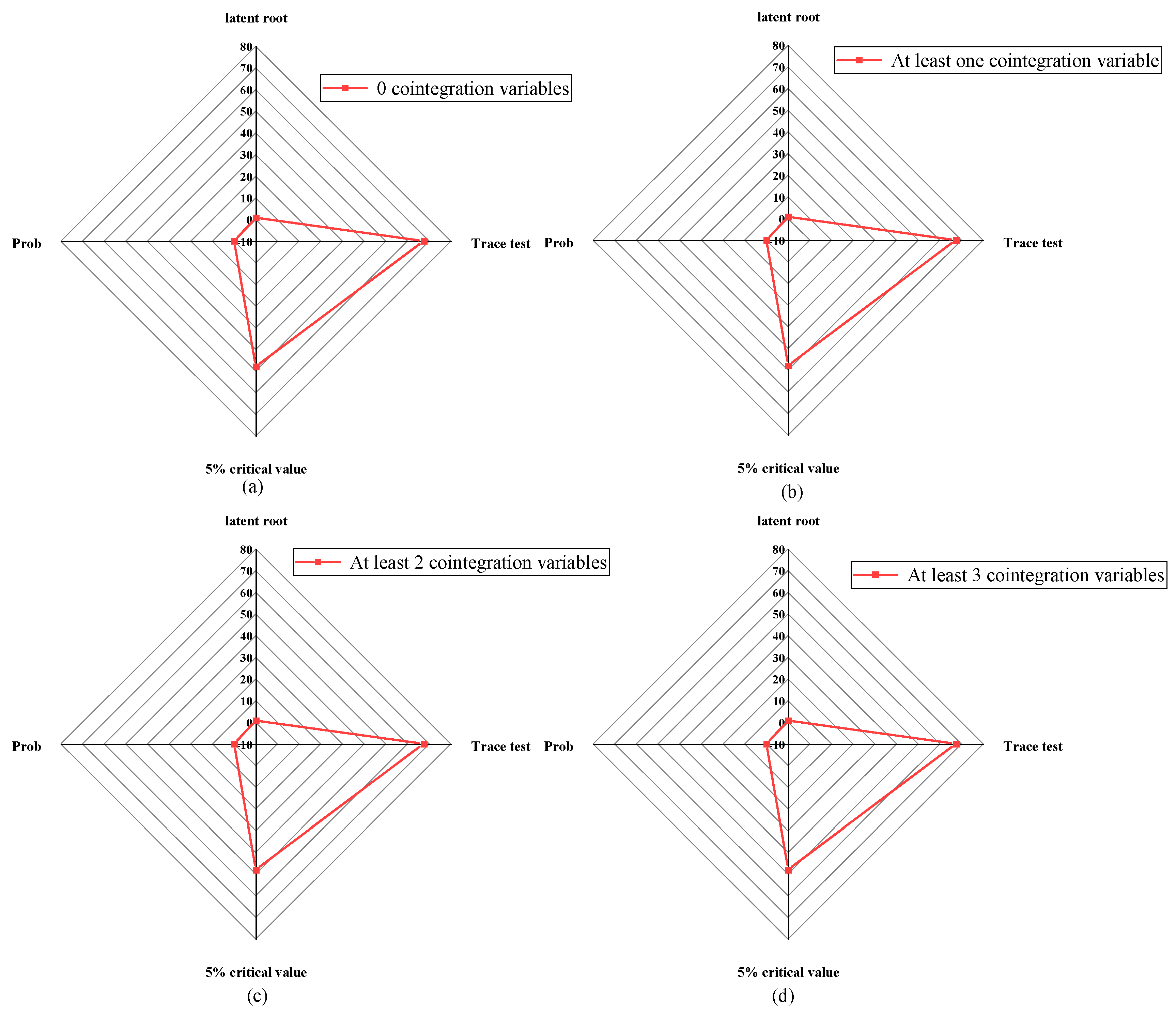
The test form (C, T, K) of lnL second-order difference and lnC second-order difference is (C, T, 1), and the remaining test forms are (M, N, 1). In the test form, C represents the constant in the test equation; T denotes the time trend; K indicates the lag order term, and N does not include the constant term or time trend term. Obviously, when the significance level is 1%, the second-order difference sequences of lnY, lnK, lnL, and lnC are stable, namely, second-order single integer. Next, the Johansen cointegration test is performed on the basic data, and the test results are shown in Figure 5.
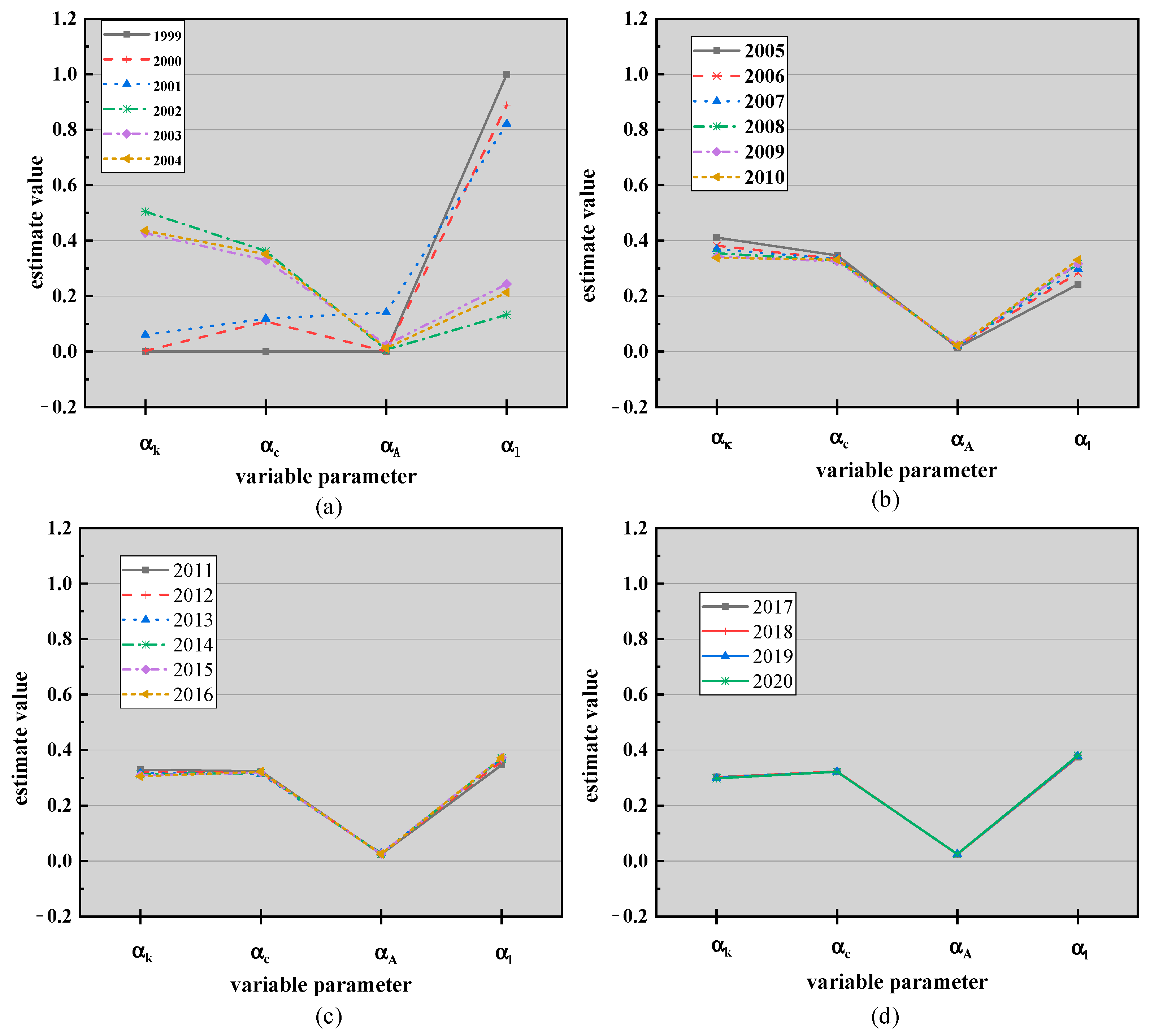
Figure 5 illustrates that when the significance level is 0.05, there are at least two cointegration variables, so the state-space model can be implemented based on the basic data. EViews is used to estimate the state-space model implemented by Equations (4)–(7), and the estimation of variable parameters α k , α c , α A can be obtained. If α k + α l + α c = 1 , that is, the return-to-scale does not change, then the estimation of α l can be obtained accordingly. The results are shown in Figure 6.
According to Figure 6, the output elasticity coefficients of labor, capital, and CO2 in Hebei Province from 1999 to 2020 can be calculated to be 0.4002, 0.3057, and 0.2941, respectively. These three data are close, indicating that labor, capital, and CO2 all play a role in promoting the economic growth of Hebei Province, and the driving effect of CO2 on the economic growth of this province is 0.2941. The results suggest that although carbon emissions have a negative impact on the environment, they can also promote economic growth to some extent. In summary, based on the calculation results in Figure 6, it can be concluded that labor, capital, and CO2 have similar promoting effects on economic growth in Hebei Province, and CO2 has a significant driving effect on economic growth. Furthermore, the test results in Figure 7 also confirm the significance of the estimated results of variable parameters and the fitting effect of the model. These research results provide an important reference and basis for economic growth and environmental protection of Hebei and can offer guidance and help for policymakers to promote the sustainable economic development of Hebei Province. Meanwhile, the estimated results of variable parameters are displayed in Figure 7. The significance of the estimated results can be found through the testing of variable parameters. Specifically, the estimated values of the output elasticity coefficients of labor, capital, and CO2 are all significantly non-zero, indicating that they significantly impact economic growth in Hebei Province. In addition, Figure 7 also shows the distribution of residual errors. It can be observed that the distribution of residual errors is relatively uniform, illustrating that the model has a better fitting effect.
In Figure 7, MSE stands for Mean Square Error, reflecting the difference between the estimator and the estimated quantity. Here, it is used to reflect the difference between the research factors and measure the value of the research results. Apparently, the MSEs of α k , α c , and α A are very small. p-values are all 0, less than 0.05. Thus, the test results are relatively significant. Additionally, ADF is employed to test the residual of the measurement equation, obtaining the p-value as 0.0355. Hence, when the significance level is 5%, the residual sequence is stable and has no unit root. The analysis result demonstrates that the estimated value is effective.

3.2.2. Estimation of Potential Outputs

Generally, the value of potential output can be estimated after the potential employment level, the potential level of capital input, and the trend total factor productivity are given. Therefore, the data of the above three aspects are calculated [36].
First, the output elasticity of labor, capital, and CO2 obtained above are taken into Equation (23), and each year’s total factor productivity level is calculated. The HP filtering method in the EViews 10.0 software is used to calculate the value of trend total factor productivity [37].
A t = Y t / K t α k t L t α l t C α c t
The potential employment level is calculated using Equation (24):
L t = L s t × T r p , t × ( 1 U t )
L t —Potential employment level, L s t —Number of employable people in terms of age, T r p , t —Proportion of labor participation, U t —Unemployment rate caused by reasons other than wages. Due to the lack of T r p , t and U t data in China, the potential employment level is difficult to estimate [38]. This work refers to the trend elimination method in relevant literature to replace some missing data. Specifically, L s t × T r p , t can be replaced by the whole economically active population, and 1 U t can be replaced by the trend component of the ratio of employed population to the economically active population in the whole province. The number of the economically active population is equal to the sum of the employed and unemployed populations. Thereby, the potential employment level is obtained [39].
The potential output and potential output growth rate of Hebei Province from 1999 to 2020 are calculated, and the results are revealed in Figure 8.
Figure 8 indicates that Hebei’s potential output has gradually increased from 1999 to 2020. By 2020, Hebei’s total potential output has reached 800 billion yuan, an increase of about eight times compared with 1999. The overall trend of potential growth is downward. With the exception of a significant rise in the potential growth rate between 2005 and 2010, the potential growth rate in other years has basically shown a downward trend. The potential growth rate after 2015 was less than 10%, and the potential growth rate in 2019 was even as low as 6.96%, reaching the lowest level in 20 years. This conclusion indicates that Hebei’s potential output has increased over time, but the growth rate has gradually slowed. Among them, the increase in potential growth rate between 2005 and 2010 may be related to policy adjustment and economic structural transformation. Since 2015, its potential growth rate has gradually declined due to multiple factors such as changes in the domestic and international economic environment and industrial transformation and upgrading. Especially in 2019, affected by domestic and international trade frictions and other factors, Hebei’s potential growth rate fell to the lowest level in 20 years. These results give important references for economic growth and policy-making in Hebei Province. By analyzing the changing trend of potential output, policymakers can formulate corresponding economic policies to promote the sustainable development of Hebei Province’s economy. At the same time, the results also provide a beneficial exploration for academic research in related fields and give theoretical support for in-depth research on China’s economic growth.
The changing trend of potential output growth rate and actual growth rate is analyzed in combination with carbon intensity, as expressed in Figure 9.
Figure 9 suggests that the trend of the actual growth rate of output in Hebei Province is basically consistent with that of the potential growth rate curve, and the values of the actual and potential growth rates are between 5–15%. This shows that the growth rate of potential output and actual output will continue to increase with the increase in carbon intensity. That is, enterprises with high carbon emissions play an important role in the economic growth of Hebei Province. In recent years, the state has paid more and more attention to environmental control, so CO2 emissions have been strictly controlled, and the actual growth rate and potential growth rate of output have decreased significantly in recent years. It shows that the economy of Hebei Province still depends on enterprises with high energy consumption and high carbon emission. When carbon emissions are controlled, it is difficult for the economy to develop better. Therefore, Hebei Province urgently needs to explore a customized green and sustainable development road to improve the economic growth rate without damaging the environment.
Next, the contribution rate of carbon emissions is utilized to measure the cost of CO2 emission in potential output. The specific calculation is:
R c = α c × r c
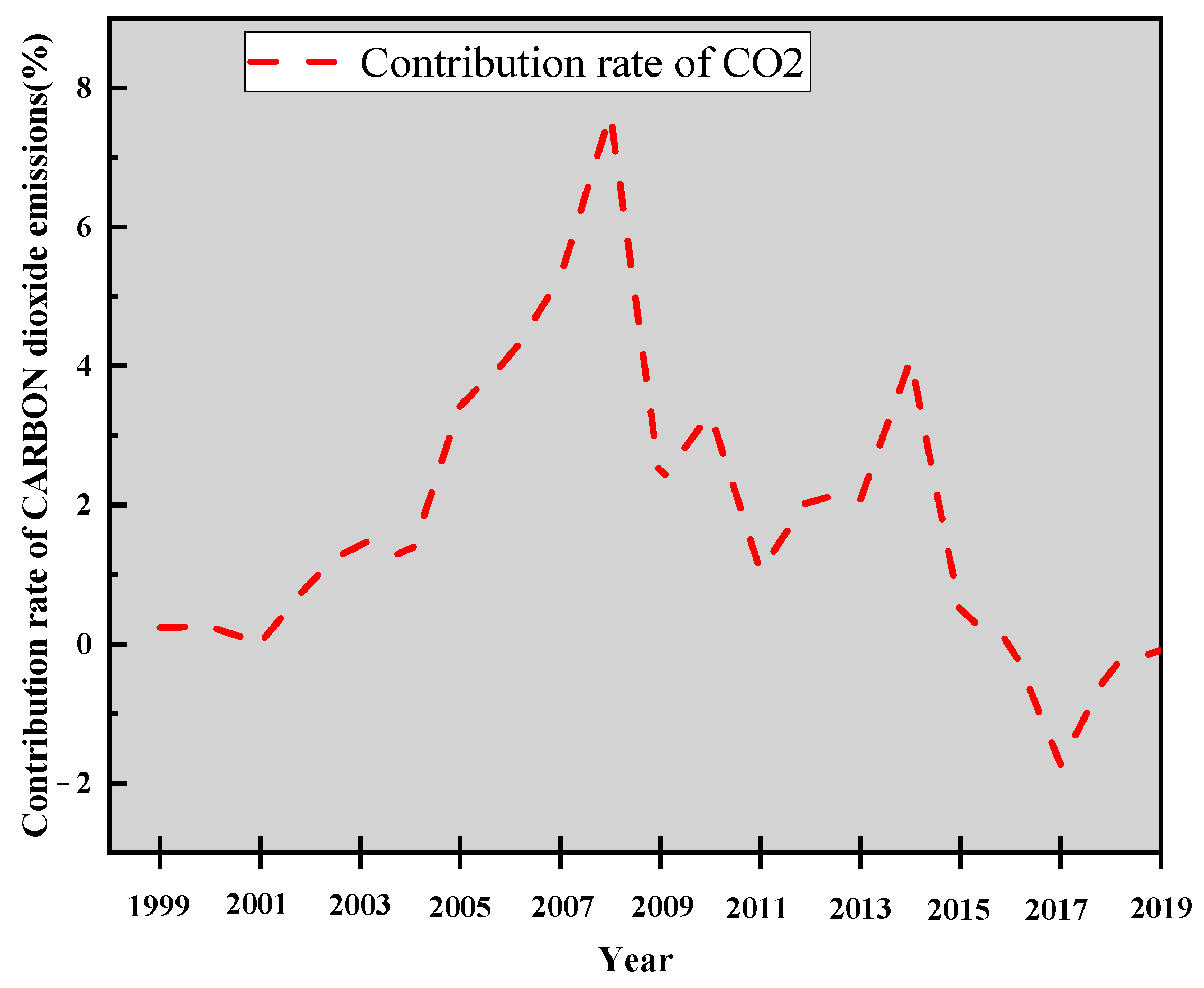
Rc—Contribution rate of carbon emissions to the economy of Hebei Province, α c —Elasticity of production, r c —Growth rate of CO2 emissions. The calculation results are presented in Figure 10.
Figure 10 illustrates that the contribution rate of CO2 emissions to the economy of Hebei Province has been increasing from 2003 to 2008, indicating that economic growth has been at the cost of damaging the environment in recent years. The contribution rate of CO2 emissions is the largest in 2009, which is.63%. After that year, the contribution rate of CO2 emissions begins to decline and even becomes negative after 2018, indicating that under the national control of the environment, the impact of CO2 emissions on economic growth is gradually reduced, which is more conducive to the sustainable development of China’s ecological environment.

3.3. Prediction of Potential Economic Growth Rate in Hebei Province under the Control of Low-Carbon Transformation

The calculation of the potential economic growth rate reads:
g t = g t f p t + α k t g k t + α l t g l t + α c t g c t
In Equation (26), the meanings of each parameter are the same as the preceding equation. The results show that labor, capital, total factor productivity, and CO2 emissions all affect the potential economic growth rate. Therefore, scenario analysis is adopted to predict the numerical changes of the potential economic growth rate of Hebei Province under the above factors and carbon emission control according to Equation (26).

3.3.1. Prediction Analysis on Changes of the Growth Rate of Various Factors

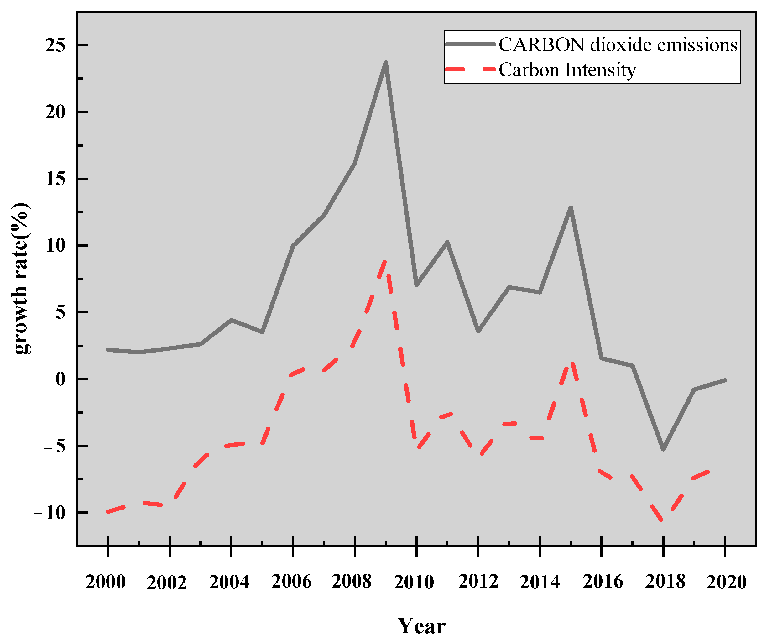
First, the growth rate of CO2 emissions is predicted. According to the Provincial carbon emission requirements, by 2025, carbon emissions will decrease by about 20% compared with 2020. It is assumed that if Hebei Province can meet the above requirements in 2024, then the potential economic growth rate of Hebei Province in the future can be predicted. Since the CO2 emissions introduced in the proposed model are slightly different from the carbon intensity in emission reduction control, it is necessary to analyze the relationship between carbon intensity and emission reduction control, as illustrated in Figure 11.
Figure 11 shows that although CO2 emission growth rate and carbon intensity growth rate are inconsistent, the changing trends of the two curves are consistent, indicating that there is a specific correlation between the two. Further, EViews is used to judge the relationship between carbon intensity growth rate and CO2 emission growth rate, and the correlation coefficient is obtained, which is as high as 0.96. Then, the logarithm of CO2 emission and carbon intensity is calculated, respectively, and the unit root is tested. The test results show that when the significance level is 1%, only the second-order difference can make the logarithmic sequence stable, and the model structure is constructed as:
ln C = 13.640 + 1.022 ln θ + 0.983 A R ( I ) + 0.937 M A ( I )
In Equation (27), ln C , ln θ —Logarithmic sequence of CO2 emission and carbon intensity. When the residual sequence of the regression equation is modified, the variable ARMA (1, 1) is introduced to eliminate the autocorrelation of the residual, and the final fitting degree of the model is as high as 0.99.
Thus, in the future, the elasticity of ln θ relative to ln C is 1.022. Then, the annual decline rate of CO2 emission must reach 4.2% to meet the requirements, while the annual decline rate of carbon intensity is 4.1%.
Second, according to the constant price of new investment in Hebei Province in the coming years, the growth rate of its capital stock is predicted. Equation (28) reveals the specific calculation of the constant price of new investment:
T r = T a × ( 1 + β )
In Equation (28), Tr—Constant price of new investment in Hebei Province every year; Ta—Constant price of fixed investment in 2020; β —Actual year-on-year growth rate. Therefore, as long as the actual year-on-year growth rate of Hebei Province is predicted, the growth rate of capital stock can be estimated.
Given the current economic situation in Hebei Province, the role of capital in promoting economic development is becoming even smaller, and the capital formation rate will continue to decline. Therefore, three scenarios, optimism, benchmark, and pessimism, are defined, which are evaluated based on 8.5% (growth rate of capital stock) in 2020. In the optimistic scenario, the actual growth rate of capital stock will remain unchanged. In the benchmark scenario, the growth rate of capital stock will continue to decline at the rate of 0.2% per year. In the pessimistic scenario the real growth rate of capital stock will decline at an annual rate of 0.5%.
Third, the growth rate of labor input is predicted. Here, a polynomial regression with time series is employed to predict the potential employment of Hebei Province and calculate the growth rate of labor input.
Fourth, the growth rate of trend total factor productivity is predicted. Through calculation, the average total factor productivity in Hebei Province from 1999 to 2020 is 1.7%. Although it decreased in 2008, the overall trend is upward. Under the new economic form of Hebei Province, the main economic driving force of this province, namely capital investment, will be replaced by innovation. The constant exploration of reform and innovation plays a major role in developing total factor productivity in Hebei Province. The trend TFP growth rate scenarios are also defined as optimism, benchmark, and pessimism. Similarly, according to the 2.4% (TFP growth rate) in 2020, the growth rate of TFP will continue to rise at the rate of 0.5% in an optimistic scenario. In the benchmark scenario, it will continue to rise at a rate of 0.2%. In a pessimistic scenario, the trend TFP growth rate will be consistent with that in 2020.
Fifth, the change in output elasticity of each factor is predicted.
According to the above prediction results of capital–output elasticity, the average value of capital–output elasticity from 2011 to 2015 was 0.318, and it decreased by 0.017 from 2016 to 2020. From this, the capital–output elasticity from 2021 to 2024 is predicted. According to the output elasticity of CO2 in the most recent three years, the output elasticity in the next few years is predicted. Under the condition that the economies of scale do not change, the output elasticity of the labor force can be calculated by Equation (29):
I B = 1 I A I C O 2
I B , I A , I C O 2 —output elasticity of labor, capital, and CO2.

3.3.2. Prediction

Finally, the potential output growth rate of Hebei Province in 2021–2024 is calculated under the three scenarios of optimism, benchmark, and pessimism. The results are exhibited in Figure 12.
To sum up, from the optimistic situation, the overall trend of potential growth rate in Hebei Province is not large. The average growth rate of the potential economy is 6.414%, while the potential growth rate in 2023 is the smallest, only 6.093%. In the benchmark scenario, Hebei’s potential growth rate is on a downward trend, falling to 5.739% by 2024. Under the pessimistic scenario, Hebei’s four-year average potential growth rate is 5.312%. This conclusion indicates that although there is some uncertainty in the future economic growth prospects of Hebei Province, it shows a gradual slowing trend on the whole. This may be related to a variety of factors, such as changes in domestic and foreign economic environment, industrial structure adjustment, and population aging. At the same time, the difference of potential growth rate in different situations also reflects the impact of different policies and market environments on economic growth. These results provide an important reference for economic planning and policy making in Hebei Province. Policymakers can formulate corresponding economic policies and development strategies according to the changing trend of potential growth rate under different circumstances, to promote the long-term and stable development of Hebei’s economy. Furthermore, these results also offer beneficial scope for academic research in related fields, and provide theoretical support for in-depth study of China’s economic growth. Compared with the study of Wang et al. (2022), this work provides a more comprehensive research scope and results, and adopts more advanced research methods to afford more advanced technologies for future development.

4. Conclusions

With the further promotion of the sustainable development concept, the green economy has become the main goal of the current social and economic system. Thus, taking Hebei Province as an example, the change trend of economic growth rate under carbon emission control is analyzed. The effects of CO2 emissions on economic growth are systematically analyzed by establishing a state-space model. The results show that the average output elasticity of labor, capital, and CO2 in Hebei Province from 1999 to 2020 are 0.4002, 0.3057, and 0.2941, respectively. Therefore, the above three factors play an important role in the economic development of Hebei Province. Among them, the driving effect of carbon emission control on the economy of Hebei Province is as high as 0.2941, indicating that the economic growth of Hebei mainly depends on enterprises with high carbon emissions. In the optimistic scenario, Hebei’s potential output growth rate will recover after a period of decline. In summary, the research conclusion shows that CO2 emissions have an important impact on the economic growth of Hebei Province, which indicates that the economic development of Hebei Province mainly depends on enterprises with high carbon emissions. Therefore, it is necessary to control carbon emissions while achieving economic growth. In addition, in the optimistic scenario, the potential output growth rate in Hebei Province will recover after a period of decline, indicating that even with strict controls on carbon emissions, the economy can still rely on high-tech for growth. The contribution of this work is to discuss the green transformation of economic growth in Hebei Province, which provides a useful reference for policymakers. At the same time, the influence of CO2 emissions on economic growth is systematically analyzed by establishing a state-space model, which gives theoretical support for academic research in related fields. Based on the research conclusions, it is suggested that policymakers should pay attention to the control of carbon emissions while promoting economic growth in Hebei Province, to achieve the balance between economic growth and environmental protection. Although the study in this work lacks detailed analysis, future explorations can study the development of the green economy in Hebei Province through more detailed content, thereby providing more theoretical support and practical guidance for promoting the sustainable development of Hebei’s economy.

Author Contributions

Conceptualization, K.C. and T.L.; methodology, S.X.; software, K.C.; validation, S.X.; formal analysis, T.L.; investigation, T.L.; resources, S.X.; data curation, K.C.; writing—original draft preparation, T.L.; visualization, S.X.; supervision, T.L.; project administration, K.C.; funding acquisition. All authors have read and agreed to the published version of the manuscript.

Funding

This research received no external funding.

Data Availability Statement

The current article content has been checked according to your instructions and the data in this article has been shared according to the URL provided.

Conflicts of Interest

The authors declare no conflict of interest.

References

  1. Hughes, T.P.; Kerry, J.T.; Álvarez-Noriega, M.; Álvarez-Romero, J.G.; Anderson, K.D.; Baird, A.H.; Babcock, R.C.; Beger, M.; Bellwood, D.R.; Berkelmans, R.; et al. Global warming and recurrent mass bleaching of corals. Nature 2017, 543, 373–377. [Google Scholar] [CrossRef]
  2. Donnelly, C.; Greuell, W.; Andersson, J.; Gerten, D.; Pisacane, G.; Roudier, P.; Ludwig, F. Impacts of climate change on European hydrology at 1.5, 2 and 3 degrees mean global warming above preindustrial level. Clim. Chang. 2017, 143, 13–26. [Google Scholar] [CrossRef] [Green Version]
  3. Sagna, K.; Amou, K.A.; Boroze, T.T.E.; Kassegne, D.; d’Almeida, A.; Napo, K. Environmental pollution due to the operation of gasoline engines: Exhaust gas law. Int. J. Oil Gas Coal. Eng. 2017, 5, 39–43. [Google Scholar] [CrossRef] [Green Version]
  4. Ali, E.B.; Anufriev, V.P.; Amfo, B. Green economy implementation in Ghana as a road map for a sustainable development drive: A review. Sci. Afr. 2021, 12, e00756. [Google Scholar] [CrossRef]
  5. Yang, Q.; Du, Q.; Razzaq, A.; Shang, Y. How volatility in green financing, clean energy, and green economic practices derive sustainable performance through ESG indicators? A sectoral study of G7 countries. Resour. Policy 2022, 75, 102526. [Google Scholar] [CrossRef]
  6. Falcone, P.M.; Hiete, M.; Sapio, A. Hydrogen economy and sustainable development goals: Review and policy insights. Curr. Opin. Green Sustain. Chem. 2021, 31, 100506. [Google Scholar] [CrossRef]
  7. Karintseva, O.; Kharchenko, M.; Boon, E.K.; Derykolenko, O.; Melnyk, V.; Kobzar, O. Environmental determinants of energy-efficient transformation of national economies for sustainable development. Int. J. Glob. Energy Issues 2021, 43, 262–274. [Google Scholar] [CrossRef]
  8. Suparjo Suparjo, S.D.; Kurniadin, N.; Kasuma, J.; Priyagus, P.; Darma, D.C.; Haryadi, H. Indonesia’s New SDGs Agenda for Green Growth–Emphasis in the Energy Sector. Int. J. Energy Econ. Policy 2021, 11, 395–402. [Google Scholar] [CrossRef]
  9. Bormann, I.; Nikel, J. How education for sustainable development is implemented in Germany: Looking through the lens of educational governance theory. Int. Rev. Educ. 2017, 63, 793–809. [Google Scholar] [CrossRef]
  10. Niu, Q.; Yu, L. Environment, development and sustainability a multidisciplinary approach to the theory and practice of sustainable development. Environ. Dev. Sustain. 2021, 22, 2069–2085. [Google Scholar] [CrossRef] [Green Version]
  11. Capra, F.; Jakobsen, O.D. A conceptual framework for ecological economics based on systemic principles of life. Int. J. Soc. Econ. 2017, 44, 831–844. [Google Scholar] [CrossRef] [Green Version]
  12. Bartkowski, B.; Lienhoop, N. Beyond rationality, towards reasonableness: Enriching the theoretical foundation of deliberative monetary valuation. Ecol. Econ. 2018, 143, 97–104. [Google Scholar] [CrossRef]
  13. Cohen, M.A.; Tubb, A. The impact of environmental regulation on firm and country competitiveness: A meta-analysis of the porter hypothesis. J. Assoc. Environ. Resour. Econ. 2018, 5, 371–399. [Google Scholar] [CrossRef] [Green Version]
  14. Leeuwen, G.; Mohnen, P. Revisiting the Porter hypothesis: An empirical analysis of green innovation for the Netherlands. Econ. Innov. New Technol. 2017, 26, 63–77. [Google Scholar] [CrossRef] [Green Version]
  15. Beşe, E.; Kalayci, S. Environmental Kuznets curve (EKC): Empirical relationship between economic growth, energy consumption, and CO2 emissions: Evidence from 3 developed countries. Panoeconomicus 2021, 68, 483–506. [Google Scholar] [CrossRef] [Green Version]
  16. Crafts, N.; Woltjer, P. Growth accounting in economic history: Findings, lessons and new directions. J. Econ. Surv. 2021, 35, 670–696. [Google Scholar] [CrossRef]
  17. Vospernik, S. Basal area increment models accounting for climate and mixture for Austrian tree species. For. Ecol. Manag. 2021, 480, 118725. [Google Scholar] [CrossRef]
  18. Harris, R.; Moffat, J. The UK productivity puzzle, 2008–2012: Evidence using plant-level estimates of total factor productivity. Oxf. Econ. Pap. 2017, 69, 529–549. [Google Scholar] [CrossRef]
  19. Svensson, A.; Schön, T.B. A flexible state–space model for learning nonlinear dynamical systems. Automatica 2017, 80, 189–199. [Google Scholar] [CrossRef] [Green Version]
  20. Ohkita, M.; Bando, Y.; Nakamura, E.; Itoyama, K.; Yoshii, K. Audio-Visual Beat Tracking Based on a State-Space Model for a Robot Dancer Performing with a Human Dancer. J. Robot. Mechatron. 2017, 29, 125–136. [Google Scholar] [CrossRef]
  21. Nowakowski, M.; Cohen, E.; Horodecki, P. Entangled histories versus the two-state-vector formalism: Towards a better understanding of quantum temporal correlations. Phys. Rev. A 2018, 98, 032312. [Google Scholar] [CrossRef] [Green Version]
  22. Delgado, M.S.; McCloud, N. Foreign direct investment and the domestic capital stock: The good–bad role of higher institutional quality. Empir. Econ. 2017, 53, 1587–1637. [Google Scholar] [CrossRef]
  23. Berlemann, M.; Wesselhöft, J.E. Aggregate capital stock estimations for 122 countries: An update. Rev. Econ. 2017, 68, 75–92. [Google Scholar] [CrossRef]
  24. Vander Donckt, M.; Chan, P.; Silvestrini, A. A new global database on agriculture investment and capital stock. Food Policy 2021, 100, 101961. [Google Scholar] [CrossRef]
  25. Dong, Q.; Murakami, T.; Nakashima, Y. Estimating China’s agricultural capital stock from 1952 to 2012. Reg. Sect. Econ. Stud. 2018, 18, 53–70. [Google Scholar]
  26. Jianu, I. The share price and investment: Current footprints for future oil and gas industry performance. Energies 2018, 11, 448. [Google Scholar] [CrossRef] [Green Version]
  27. Aganbegyan, A.G. Investments in fixed assets and human capital: Two interconnected drivers of socioeconomic growth. Stud. Russ. Econ. Dev. 2017, 28, 361–363. [Google Scholar] [CrossRef]
  28. Hartwig, J. “Relative movements of real wages and output”—How does Keynes’s 1939 essay relate to his theory of effective demand? J. Hist. Econ. Thought 2017, 39, 257–270. [Google Scholar] [CrossRef] [Green Version]
  29. Khalil, A.; Rajab, Z.; Amhammed, M.; Asheibi, A. The benefits of the transition from fossil fuel to solar energy in Libya: A street lighting system case study. Appl. Sol. Energy 2017, 53, 138–151. [Google Scholar] [CrossRef]
  30. Santosa, P.I.; Pranatal, E. Study of emission quantification in catamaran fishing vessels based on fossil energy. J. Phys. 2021, 1833, 012042. [Google Scholar] [CrossRef]
  31. Cozzi, G. Endogenous growth, semi-endogenous growth... or both? A simple hybrid model. Econ. Lett. 2017, 154, 28–30. [Google Scholar] [CrossRef] [Green Version]
  32. Gupta, R.; Stander, L. Social Status, Inflation and Endogenous Growth in A Cash-in-Advance Economy: A Reconsideration using the Credit Channel. Manch. Sch. 2018, 86, 622–640. [Google Scholar] [CrossRef] [Green Version]
  33. Liu, Y.; Xu, R.X.; Zhang, H.D.; Yan, Y. Dissipaton equation of motion theory versus Fokker-Planck quantum master equation. Chin. J. Chem. Phys. 2018, 31, 245. [Google Scholar] [CrossRef] [Green Version]
  34. Petrescu, F.I.T. Machine motion equations at the internal combustion heat engines. Am. J. Eng. Appl. Sci. 2015, 8, 127. [Google Scholar] [CrossRef]
  35. Bartosik, K.; Mycielski, J. The output employment elasticity and the increased use of temporary contracts: Evidence from Poland. Acta Oecon. 2020, 70, 83–104. [Google Scholar] [CrossRef]
  36. Oliveira, F.N.; Petrassi, M. Do financial crises erode potential output? A cross-country analysis of industrial and emerging economies. J. Econ. Stud. 2018, 45, 247–262. [Google Scholar] [CrossRef]
  37. Li, B.; Zhu, X. Forecast of maize production in Henan province. Am. J. Plant Sci. 2018, 9, 2276–2286. [Google Scholar] [CrossRef] [Green Version]
  38. Teguh, M.; Bashir, A. Indonesia’s Economic Growth Forecasting. Sriwij. Int. J. Dyn. Econ. Bus. 2019, 3, 134–145. [Google Scholar] [CrossRef]
  39. Wang, L.; Wang, Y.; Sun, Y.; Han, K.; Chen, Y. Financial inclusion and green economic efficiency: Evidence from China. J. Environ. Plan. Manag. 2022, 65, 240–271. [Google Scholar] [CrossRef]
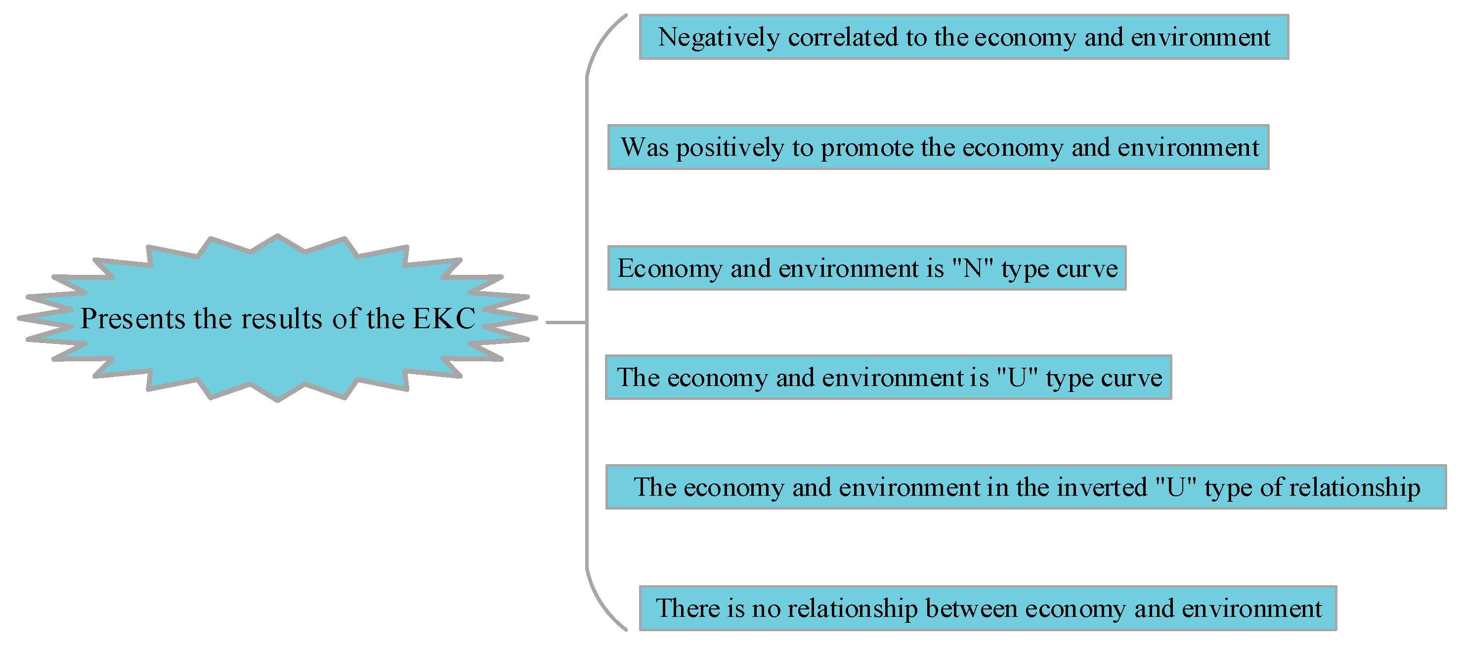
Figure 1. The results of EKC.
Sustainability 15 10145 g001
Figure 2. Changes of capital stock in different initial settings relative to 1.6 times of initial settings.
Sustainability 15 10145 g002
Figure 3. Average low calorific value and CO2 emission coefficient of various energy sources ((a): IPCC CO2 emission coefficient; (b): Average low calorific value; (c): CO2 emission coefficient).
Sustainability 15 10145 g003
Figure 4. ADF test results ((a): ADF statistics; (b): 1% threshold; (c): 5% threshold; (d): 10% threshold).
Sustainability 15 10145 g004
Figure 5. Johansen cointegration test results ((a): 0 cointegration variables; (b): At least one cointegration variable; (c): At least 2 cointegration variables; (d): At least 3 cointegration variables).
Sustainability 15 10145 g005
Figure 6. Estimation results of variable parameters ((a): Estimation of variable parameters from 1999 to 2004; (b): Estimation of variable parameters from 2005 to 2010; (c): Estimation of variable parameters from 2011 to 2016; (d): Estimation of variable parameters from 2017–2020).
Sustainability 15 10145 g006
Figure 7. Test results of variable parameters ((a): Inspection results of α k ; (b): Inspection results of α c ; (c): Inspection results of α A ).
Sustainability 15 10145 g007
Figure 8. Timing chart of potential output and potential growth rate in Hebei Province ((a): Timing chart of potential outputs; (b): Timing chart of potential growth rate).
Sustainability 15 10145 g008
Figure 9. Timing chart of carbon intensity and actual and potential growth rate in Hebei Province.
Sustainability 15 10145 g009
Figure 10. Contribution rate of CO2 emissions.
Sustainability 15 10145 g010
Figure 11. The changing trend of the growth rate of CO2 emissions and carbon intensity.
Sustainability 15 10145 g011
Figure 12. Prediction of potential output growth in Hebei Province from 2021 to 2024 under different scenarios((a): Prediction of capital, labor, CO2, and TFP growth rate; (b): Prediction of labor, capital, CO2, and potential growth rate).
Sustainability 15 10145 g012
Disclaimer/Publisher’s Note: The statements, opinions and data contained in all publications are solely those of the individual author(s) and contributor(s) and not of MDPI and/or the editor(s). MDPI and/or the editor(s) disclaim responsibility for any injury to people or property resulting from any ideas, methods, instructions or products referred to in the content.