Article

A Convolution–Non-Convolution Parallel Deep Network for Electricity Theft Detection

1
School of Materials Science and Engineering, Northeastern University, Shenyang 110819, China
2
College of Information Science and Engineering, Northeastern University, Shenyang 110819, China
*
Author to whom correspondence should be addressed.
Sustainability 2023, 15(13), 10127; https://doi.org/10.3390/su151310127
Submission received: 19 May 2023 / Revised: 12 June 2023 / Accepted: 20 June 2023 / Published: 26 June 2023
(This article belongs to the Section Energy Sustainability)

Abstract

:
This paper proposes a novel convolution–non-convolution parallel deep network (CNCP)-based method for electricity theft detection. First, the load time series of normal residents and electricity thieves were analyzed and it was found that, compared with the load time series of electricity thieves, the normal residents’ load time series present more obvious periodicity in different time scales, e.g., weeks and years; second, the load times series were converted into 2D images according to the periodicity, and then electricity theft detection was considered as an image classification issue; third, a novel CNCP-based method was proposed in which two heterogeneous deep neural networks were used to capture the features of the load time series in different time scales, and the outputs were fused to obtain the detection result. Extensive experiments show that, compared with some state-of-the-art methods, the proposed method can greatly improve the performance of electricity theft detection.

1. Introduction

Electricity theft is the use of various methods to reduce the payment of electricity charges and achieve illegal benefits. Electricity theft detection is of great significance to ensure the safety and stability of a power system, and, at present, much attention has been paid to the modeling and detection of electricity theft [1]. Electricity theft detection can be completed by adding special hardware on the user side; however, this would significantly increase the system and maintenance cost. Meanwhile, electricity thieves can also avoid detection by tampering with the hardware. Therefore, currently, most efforts that have been made on electricity theft detection are based on electricity consumption data analysis [2,3].
Electricity theft detection is a very challenging issue as there are many ways to steal electricity; meanwhile, electricity theft may not occur continuously [4,5]. Based on the different detection principles, current electricity theft detection methods can be divided into two types: short-period-comparison-based electricity theft detection methods and whole-period-classification methods. Short-period-comparison-based electricity theft detection methods generally adopt anomaly detection methods based on a sliding time period window, and Table 1 gives some typical short-period-comparison-based electricity theft detection methods. The main assumption is that the electricity theft of an electricity thief only occurs in parts of periods, and that the electricity theft behaviors would change the distribution of electricity consumption data significantly. Therefore, for the beginning of the electricity consumption profile, if some features of electricity consumption data in the current time period window are obviously different from those in the previous time period window, it can be considered that electricity theft has occurred. For example, in [6,7], if the mean value and variance of the data in the current time period window change significantly compared with the previous window, it is considered that there is electricity theft. In [8,9], autoencoders are trained using the normal data, and if the reconstruction error of the data in the current time period window on the trained autoencoder is abnormally large, it is considered that there is electricity theft. In [10,11], if the electricity consumption data in the current time period window do not belong to the same cluster as the data in the previous time period window, it is considered that there is electricity theft. In [12], if the correlation between the electricity consumption data in the current time period window and in the previous window is low, it is considered that there is electricity theft. Jokar et al. [13] modeled a variety of typical electricity theft patterns, and if the electricity consumption data in the current time period window conform to a certain theft pattern, it is considered that there is electricity theft. The advantage of the short-period-comparison-based methods is that they can identify the occurrence time of electricity theft. However, due to the complexity of the electricity consumption data of normal users, as well as the diversity of electricity theft methods, electricity theft data and normal consumption data can generally only be effectively distinguished using long-time-period data. Because the features used in short-period-comparison-based methods may not change significantly in the actual scenes, such methods are usually verified on simulated datasets, as shown in Table 1.
Due to the above reasons, current research mainly focuses on electricity theft detection based on the whole period data, which can be regarded as a binary classification problem. According to the classification process, whole-period-classification methods can be divided into two types: two-stage methods and one-stage methods, Table 2 and Table 3 give some state-of-the-art two-stage and one-stage whole-period-classification methods, respectively. The two-stage methods consist of two procedures: feature extraction and feature-based classification [14]. For example, ref. [15] uses seven networks for feature extraction and one discrimination network for classification. Ref. [16] uses breakout detection for feature extraction and an SVM for classification. Ref. [17] uses six feature extraction methods for feature extraction and XGBoost for classification. Ref. [18] uses discrete wavelet transform for feature extraction and random undersampling boosting for classification. Ref. [19] is a special two-stage detection method. It uses the decision tree for feature extraction, but inputs all the original data together with the result of the decision tree into an SVM for theft detection; therefore it can be regarded as a 1.5-stage detection method. The procedure of feature extraction affords the two-stage whole-period-classification methods better interpretability; however, in addition to the performances of feature extraction algorithms and electricity theft classification algorithms, the effectiveness of the extracted features also determines the accuracy of theft detection [20]. Different from two-stage methods, one-stage methods identify electricity theft based on the data directly. Many one-stage methods employ a single classifier, such as support vector description [21], LightGBM [22,23], XGBoost [23,24], long short-term memory (LSTM) [25], deep vector embedding [26], Bayesian risk framework [27], linear regression [28], the black hole algorithm [29], random forest [30], feed forward neural networks [31], TripleGAN [32], etc. Note that [30,31,32] use a stacked autoencoder, deep autoencoder, and relational autoencoder for features extraction, and then use a random forest, feed forward neural networks, and TripleGAN for classification. However, because the main function of the autocoder is dimensionality and noise reduction, which can be regarded as a data preprocessing process, [30,31,32] are still regarded as one-stage algorithms in this paper. Meanwhile, some of the one-stage methods fuse a multi-classifier to further improve the performance of the detection methods. For example, ref. [33] uses LSTM and multi-layer perceptrons (MLPs), ref. [34] uses the maximum information coefficient and fast search and find of density peaks, and [35] uses a back propagation neural network (BP) and convolutional neural networks (CNNs). Compared with two-stage detection methods, one-stage whole-period-classification algorithms avoid the possibility of reducing the detection accuracy caused by inappropriate feature extraction. However, as end-to-end methods, the interpretability of one-stage whole-period-classification algorithms is reduced, and the generalization ability of the algorithm may decline.
Although currently there are many electricity theft detection methods, as shown in Table 1, Table 2 and Table 3, because of the difficulties in collecting large-scale real electricity theft data, most of these methods use simulated theft data generated according to the specific electricity theft pattern. Due to the lack of real electricity theft data, few of these works fully consider the features of normal and theft data, and most of them regard electricity theft detection as a general classification or abnormal detection problem, which limits the performance of the detectors.
This paper proposes a novel one-stage whole-period-classification method: a convolution–non-convolution parallel deep network (CNCP)-based method for electricity theft detection. First, similar to one-stage electricity theft detection algorithms, the proposed CNCP method avoids the possibility of reducing the detection accuracy caused by inappropriate feature extraction. Second, in some previous studies [36,37], it was found that, influenced by work statuses and living habits, the electricity consumption of normal residents usually fluctuates on a one-week cycle. Meanwhile, through data analysis in Section 2.3 and Section 2.4, it can be seen that the periodic feature of the electricity consumption of electricity theft users is weaker than those of normal users, and, after converting temporal data into 2D image data based on a certain period, such a difference becomes more obvious. On this basis, the proposed CNCP structure can effectively capture the features of the electricity consumption time series locally and globally simultaneously, and can therefore obtain much better detection results compared with state-of-the-art methods. The contribution of this paper can be summarized as follows:
  • The features of the electricity consumption time series of normal users and electricity thieves were analyzed, and it was found that compared with those of electricity thieves, the electricity consumption time series of normal users have more obvious periodic characteristics;
  • A novel CNCP-based method for electricity theft detection was proposed in which two heterogeneous deep neural networks were used to capture the features of the electricity consumption time series in different time scales effectively, therefore yielding better detection results.
The rest of this paper is organized as follows: Section 1 gives the related works, Section 2 gives the data set description and the data preprocessing method, Section 3 first presents the electricity consumption features of normal users and electricity thieves and then the proposed CNCP-based electricity theft detection method, and Section 4 and Section 5 are the experiments and the conclusions.

2. Materials and Methods

2.1. Dataset

In Table 1, Table 2 and Table 3, typical state-of-the-art electricity theft detection methods are summarized. It can be seen that, although currently there are many electricity theft detection methods, most of them use simulated theft data, and the available public real electricity theft dataset is the dataset released by the State Grid Corporation of China (SGCC). The reason comes from the fact that electricity data usually have strong privacy; meanwhile, it is very difficult to collect large-volume real theft data. For the study on electricity theft detection, although theft data can be simulated according to some specific features of electricity theft behaviors, these simulated data are far away from the real theft data.
In this paper, the SGCC dataset was used for electricity theft detection [38]. The SGCC dataset contains daily total electricity consumption time series of 42,373 users from 1 January 2014 to 1 October 2016, totalling 1036 days. In this dataset, 3615 are electricity thieves confirmed by on-site electricians. Each electricity consumption time series is labeled by 1 or 0 to indicate if it is from an electricity thief or not. Note that there is no label to indicate when electricity theft occurs or stops. Meanwhile, no other information is available, such as the location of the user, weather information, etc. Electricity theft detection on this dataset can be considered as a binary classification problem. It is the determination of whether a resident is an electricity thief or not only based on the daily total electricity consumption time series during the whole data collection period.

2.2. Data Preprocessing

In the dataset, there are some 0 or invalid elements, which are brought in by the failure of data collection and transmission. In this paper, first, 0 or the invalid elements in each user’s load profile are counted. When its ratio to the whole load profile of the specific user is greater than 30%, this load profile is discarded. Through this operation, 33,130 valid electricity consumption time series are retained, in which 2045 (6.17%) are from electricity thieves.
Second, a two-directional weighted interpolation method is designed to correct remaining 0 and invalid elements. For an electricity consumption time series X = x i , it is first reshaped into a W × 7 matrix, where W is the number of weeks.
Ψ = . . . x i w 3 . . . . . . x i w 2 . . . . . . x i w 1 . . . x d 3 w x d 2 w x d 1 w x i w x d + 1 w x d + 2 w x d + 3 w . . . x i w + 1 . . . . . . x i w + 2 . . .
If x d w = 0 or is invalid, when it is a workday, it is replaced by:
x ˜ d w = λ 1 x d d 1 w + λ 2 x d + d 2 w + λ 3 x d w w 1 + λ 4 x d w + w 2
λ 1 = 1 3 d 1 3 d 1 + d 2 + w 1 + w 2
λ 2 = 1 3 d 2 3 d 1 + d 2 + w 1 + w 2
λ 3 = 1 3 w 1 3 d 1 + d 2 + w 1 + w 2
λ 4 = 1 3 w 2 3 d 1 + d 2 + w 1 + w 2
where x d d 1 w and x d + d 2 w are the first valid data before and after x d w ; d 1 and d 2 are the interval days; x d w w 1 and x d w + w 1 are the first valid data above and below x d w along the column direction in Ψ ; w 1 and w 2 are the interval weeks, respectively. If x d d 1 w is invalid, then d 1 = d 2 , x d d 1 w = x d + d 2 w , and vice versa. For x d w w 1 and x d w + w 2 , it is similar to x d d 1 w and x d + d 2 w .
When x d w is on weekend, it is replaced by:
x ˜ d w = λ 3 x d w w 1 + λ 4 x d w + w 2
λ 3 = w 2 w 1 + w 2
λ 4 = w 1 w 1 + w 2
If x d d 1 w is invalid, then w 1 = w 2 , x d w w 1 = x d w + w 2 , and vice versa.
Third, all data are normalized by:
x ^ = x x min x max x min
where x max and x min are maximum and minimum load of a certain user.

2.3. Analysis of Electricity Consumption Features of Normal Residents and Electricity Thieves

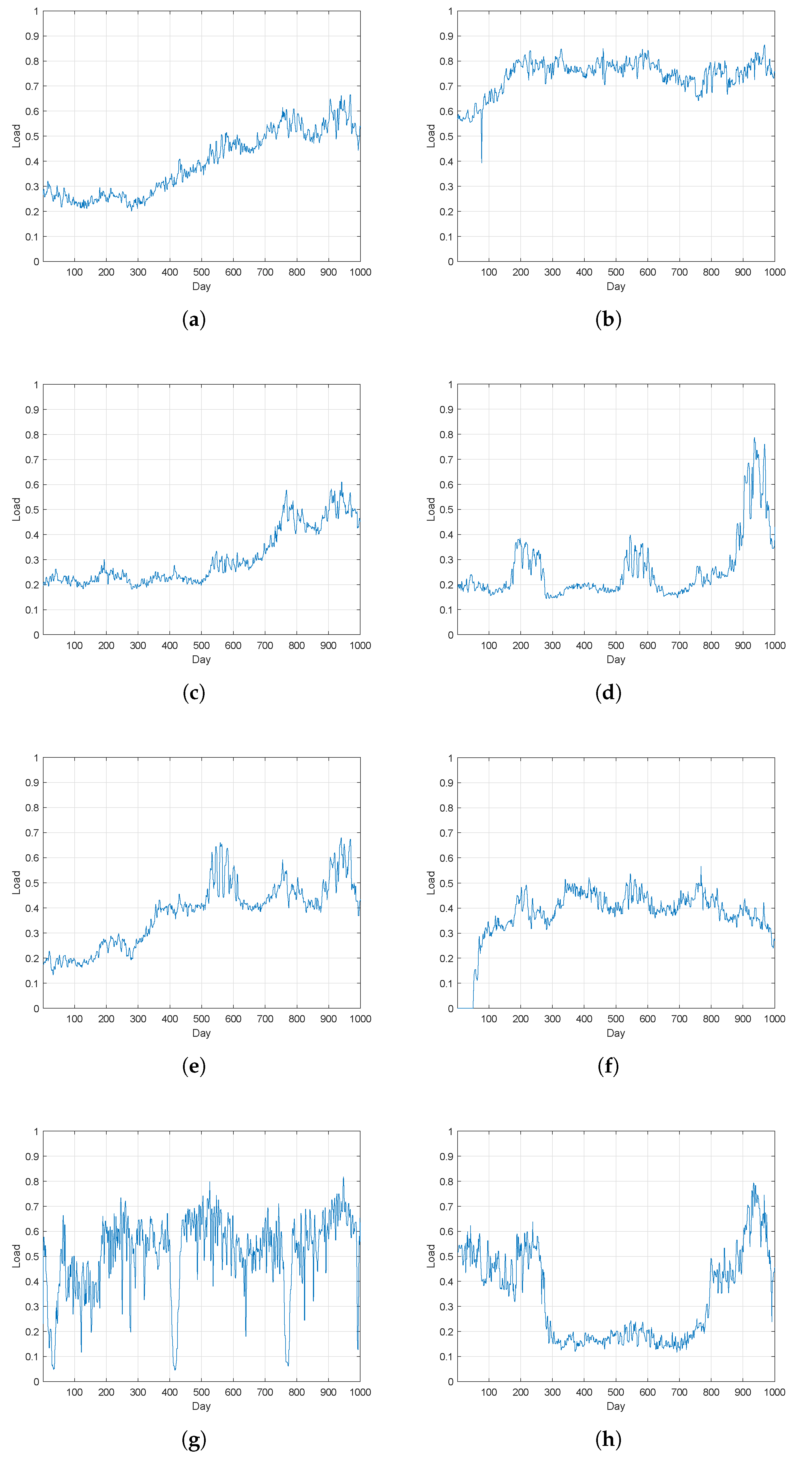
To understand the difference between normal residents and electricity thieves, the load profiles of normal residents and electricity thieves are clustered, respectively, to obtain the main consumption patterns of them. In detail, for the electricity consumption time series of normal residents, first the k-means method was adopted for data clustering using the k-means function in Matlab. As the number of patterns is unknown, we gradually increased the number of clusters until similar patterns were divided into two clusters. Finally, the number of clusters was set to 10, and the two clusters with smallest number of samples were considered as noises and ignored. Figure 1 and Figure 2 give the clustering results of the loads of normal users and electricity thieves.
As shown in Figure 1, for normal residents, all load patterns present obvious periodicity, and are closely related to the outdoor temperature. Most of the patterns are relatively stable, and only a few of them show an overall upward trend. However, the trend is smooth without sudden change. For example, the peaks and valleys of pattern (a), pattern (b), pattern (c), pattern (e) and pattern (f) are stable and consistent with the outdoor temperature. And for pattern (d), pattern (g) and pattern (h), although the overall trends of them are upward, the peaks and valleys are still consistent with the outdoor temperature, indicating that these users mainly use electric equipment such as air conditioners to adjust the room temperature in summer.
However, as shown in Figure 2, for electricity thieves, most of the patterns have little correlation with the outdoor temperature, and some of them change dramatically. For example, pattern (a), pattern (c), and pattern (d) increase dramatically after day 500. Pattern (b), pattern (g), and pattern (h) are very complex and have little relationship with the outdoor temperature.
From the above analysis, it is clear that, compared with the load time series of electricity thieves, the normal residents’ load time series present more obvious periodicity.

2.4. A Novel CNCP-Network-Based Detection Method

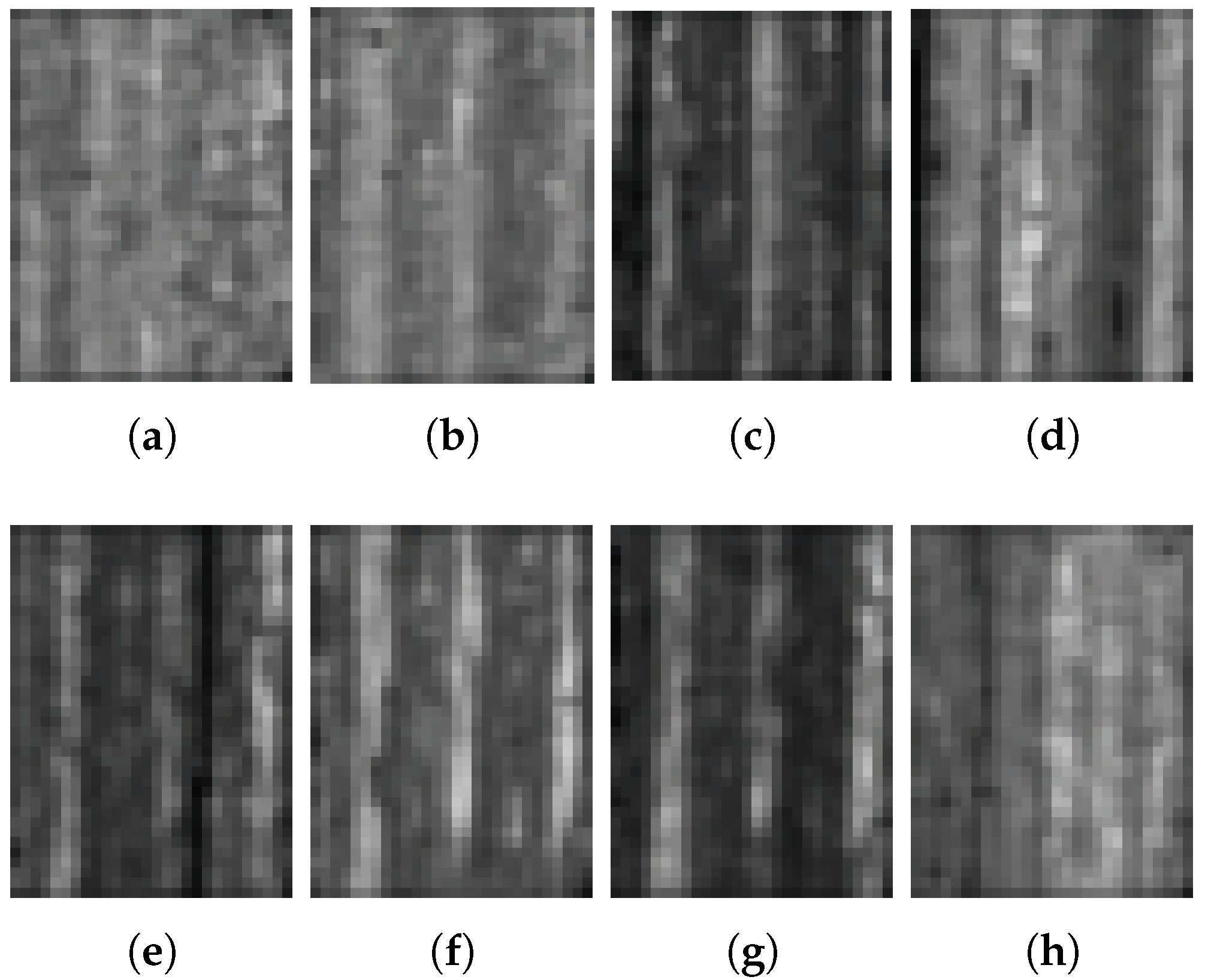
As shown in Figure 1 and Figure 2, as well as the analyses in Section 1, normal residents and electricity thieves would be classified effectively from the viewpoint of image classification. Therefore, in this paper, first, the original electricity consumption time series were converted into 2D images according to the periodicity, and then a specific image classification method was designed to distinguish normal residents and electricity thieves. Figure 3 and Figure 4 are the converted images in accordance with Figure 1 and Figure 2. In detail, first, the original electricity consumption time series (1 × 1036) was reshaped to a 37 × 28 matrix using the reshape function in Matlab, and then the matrix was rescaled into the range of 0 and 255: I = r o u n d ( I / m a x ( I ) ) × 255 . The advantages of the set of the size of the matrix are that, first, the corresponding image directly reflects the periodicity of the time series as each row of the matrix consists of successive four-week consumption data; second, the width and the height of the matrix are close to each other, which would be beneficial to the performance of the image classification method. From Figure 3 and Figure 4, it can be seen that, for normal residents, intensities of the images show relative periodicity. However, as shown in Figure 4, for electricity thieves, such periodicity is much weaker and the distributions of intensities of images are more complex.
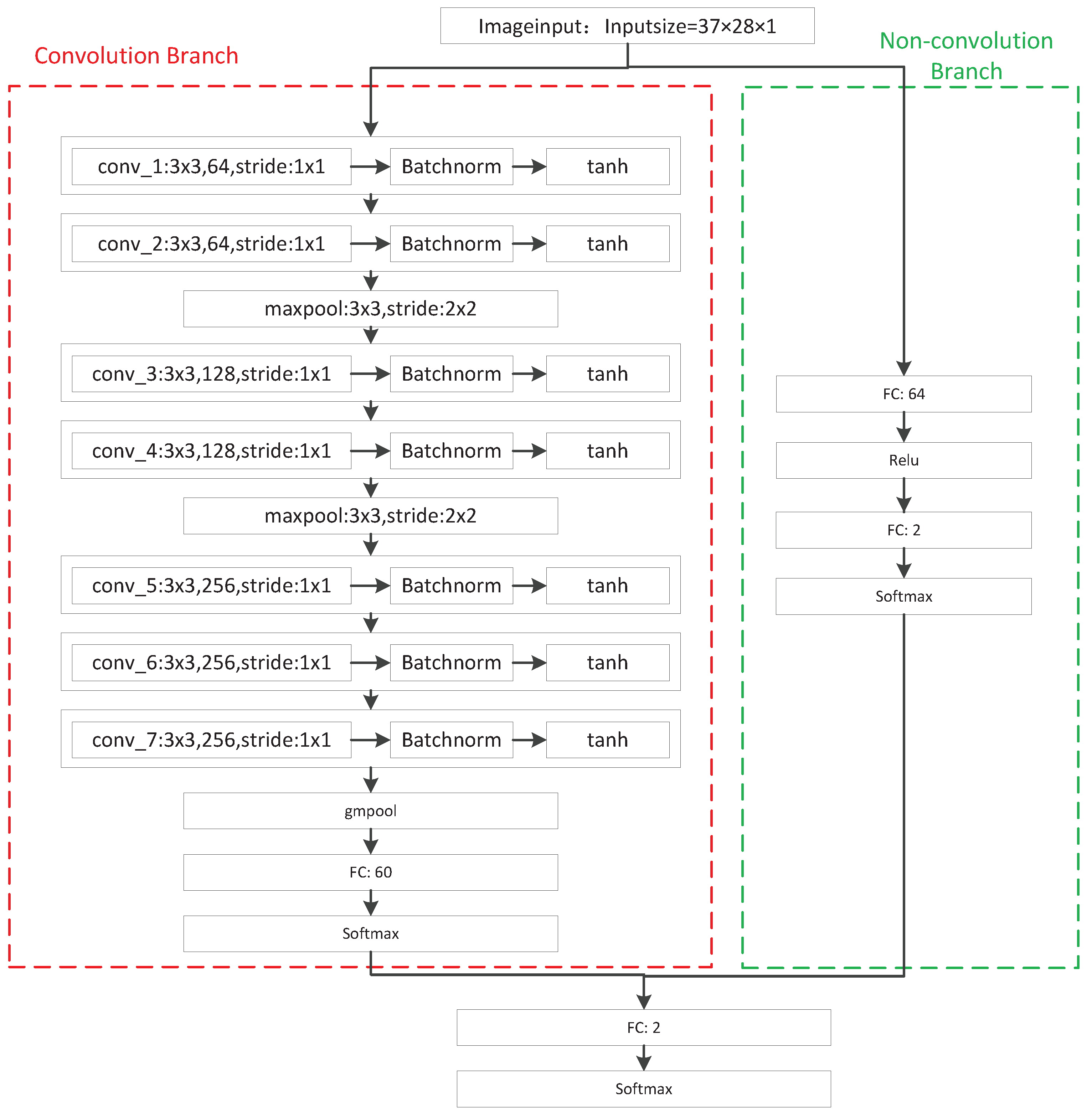
Second, a novel parallel-network-based electricity theft detection method was proposed for electricity theft detection that consists of a convolution deep branch and a non-convolution deep branch, and the results from the two branches were finally fused by a fully connected layer and a softmax layer. The overall structure of the proposed detection method can be seen in Figure 5.
To determine an optimal structure for the proposed method, a series of backbone networks were tested, which are listed in Table 4. This paper aimed to examine the impact of networks with different depths on classification results in order to select a network suitable for the problem of electricity theft detection. Through experiments, it was found that VGG series networks [39] have good performance for the convolutional branch. Therefore, this paper selected three types of VGG networks, namely VGG11, VGG13, and VGG16, where the number represents the depth of the network. Meanwhile, we designed fully-connected-layers-based networks with different depths for the non-convolutional branch. These networks are composed of fully connected layers and softmax layers, and the neurons in the fully connected layer increase with the number of layers. An example structure of the proposed detection method based on C1-N1 is given in Figure 6. As shown in Figure 6, there are two branches in the proposed method: one is a convolution branch, and the other is a non-convolution branch. In Figure 6, the convolution branch adopts the VGG11 structure, which consists of 7 convolutional layers, a gmpool layer, a fully connected (FC) layer, and a softmax layer. Each convolutional layer is followed by a batchnorm block and a tanh function. Meanwhile, two maxpool layers are inserted between the second and the third convolutional layers, as well as the fourth and the fifth convolutional layers, respectively. The non-convolution branch consists of two FC layers, a relu block, and a softmax layer. Finally, the two branches are fused by a FC layer, and a softmax layer is used as the output. The parameters of all blocks can be found in Figure 6.
The proposed method mainly consists of convolutional layers, pooling layers, FC layers, and the loss function. Data forward propagation between convolutional layers can be expressed by:
z i , j , k l + 1 = s , m , n a s , ( j 1 ) d + m , ( k 1 ) d + n l w i , s , m , n l + 1 + b i l + 1
a i , j , k l + 1 = tanh z i , j , k l + 1
where z and a are the input and the output of a neuron, l is the index of a layer, s is the number of feature maps, ( j , k ) is the index of the entry of a feature map, w is the weight, i is the number of neurons in the next layer, ( m , n ) is the the index of the entry of the convolutional kernel, b is the bias, and d is the strike step.
During the error back–forward propagation between convolutional layers process, as the parameter-updating rules of neural network are based on gradient descent methods, the gradient of any parameter θ can be obtained by:
θ t + 1 = θ t η ( L o s s ) θ t
For a max pooling layer:
p i , j , k l = max m , n a i , ( j 1 ) d + m , ( k 1 ) d + n l
where p is the output of a max pooling layer, d is the strike step, and ( m , n ) is the index of the entry of the max pooling layer.
In the proposed network, binary cross entropy was used as the loss function:
L = 1 N i = 1 N y i · log p y i + 1 y i · log 1 p y i
where y is the label of the ground truth, 1 or 0 indicates positive or negative, and p ( y ) is the possibility that the sample is predicted to be positive.
During the training process, the error of a FC layer can be calculated by:
δ j l C z j l
The error of a convolutional layer can be calculated by:
δ j L C z j L = C a j L σ z j L
where C is the forward error and σ is the activation function.

2.5. Solution of Imbalance Data

After the preprocessing step in Section 3, in the whole dataset, 33,130 valid load time series remain, including 2045 (6.17%) samples of electricity theft. If using these load time series to train a classifier, the bias will be great as the items in different classes are extremely imbalanced. In this paper, a re-sampling method was designed to balance the items in different classes. In Section 3, eight main patterns of electricity thieves are obtained. To generate a new electricity thief load time series, first, a pattern P of electricity theft was randomly selected, then two samples p 1 and p 2 belonging to P were randomly selected, and a new sample p ^ was generated using:
p * = w × p 1 + ( 1 w ) × p 2
p ^ = p * p * min p * max p * min
where p * max and p * min are maximum and minimum of p * , and w is a weight randomly drawn in the range of 0 and 1.
The above sample generation process was repeated until the number of load time series of electricity theft was equal to that of the normal residents.

3. Results

In this section, two groups of experiments are carried out. In the first group of experiments, a series of backbone networks were adopted in the proposed convolution–non-convolution parallel deep network method in order to obtain a optimal structure. In the second group of experiments, the proposed method was compared with several widely used and state-of-the-art methods. During the training process, 80% of the samples were randomly selected as the training set, and the rest were used as the test set, and the total number of training iterations was 7000. The experiments were carried out on a server with rtx2080ti, and the development environment was matlab2020a. Four performance indicators were recorded, including the true positive (TP), false positive (FP), true negative (TN), and false negative (FN). Then, P r e c i s i o n , R e c a l l , and F 1 S c o r e were obtained by:
P r e c i s i o n = T P T P + F P
R e c a l l = T P T P + F N
F 1 S c o r e = 2 × P r e c i s i o n × R e c a l l P r e c i s i o n + R e c a l l
where T P is the number of correctly detected electricity thieves, T N is the number of correctly detected normal users, F P is the number of mistakenly detected normal users, F N is the number of mistakenly detected electricity thieves, T P + F N is the total number of electricity thieves, F P + T N is the total number of normal users, and T P + T N is the total number of correctly detected users (including correctly detected electricity thieves and correctly detected normal users). The performance of a method is mainly judged by F 1 S c o r e , especially when P r e c i s i o n and R e c a l l are inconsistent.

3.1. Optimal Structure Determination

In this section, to obtain a optimal structure, a series of backbone networks are tested in the proposed method, which are shown in Table 4. During the training process, binary cross entropy was used as the loss function, and He-initialization was used as the weights initializer; the optimizer was sgdm, and its momentum was 0.9; L2 regularization was 0.0001, the batch size was 128, the initial learning rate, drop factor, and drop period were 0.001, 0.1, and 10, respectively; and when the accuracy of the verification set did not increase within the last five epochs, the training was stopped. The results are shown in Table 5. In Table 5 and the tables in rest of this paper, the red color is used to indicate the best result of the corresponding evaluating indicator.
In Table 5, C1, C2, and C3 are the results using a single convolution branch, and can be considered as general deep convolution neural networks. N1, N2, N3, N4, and N5 are the results using a single non-convolution branch, and can be considered as general deep neural networks. From Table 5, it can be seen that, when using a single convolution branch, C2 can obtain the best performance. As, from C1 to C3, the network complexity increases, it can be considered that C1 suffers from over-fitting whereas C3 suffers from under-fitting. Meanwhile, when using a single non-convolution branch, N3 has the best performance. Similar to the analysis on the results using a single convolution branch, it can be considered that N1 and N2 suffer from over-fitting whereas N4 and N5 suffer from under-fitting. Note that the result of C2 is better than that of N3, meaning that the convolutional layer can indeed extract the feature of the load time series effectively. For the proposed method, results of nine different combinations are given; that is, C1+N1, C1+N2, C1+N3, C2+N1, C2+N2, C2+N3, C3+N1, C3+N2, and C3+N3. We ignored N4 and N5 as their performance was obviously worse than N1, N2, and N3. The convolution branch of the algorithm proposed in this paper used the classical VGG network, and its convolution kernel was 3 × 3 . To test the influence of the filter size on the proposed method, the revised paper gives the detection results using 5 × 5 convolution kernels and 7 × 7 convolution kernels. In Table 5, C2(3)+N3 gives the results of the CNCP network with 3 × 3 convolution kernels, C2(5)+N3 gives the results of the CNCP network with 5 × 5 convolution kernels, and C2(7)+N3 gives the results of the CNCP network with 7 × 7 convolution kernels.
From Table 5, it can be seen that the performance of methods using 5 × 5 convolution kernels and 7 × 7 convolution kernels is similar, but lower than the proposed method using 3 × 3 convolution kernels. This is consistent with the analysis of the proponents of VGG network; that is, two 3 × 3 convolution kernels can replace one 5 × 5 convolution kernel, and three 3 × 3 convolution cores can replace one 7 × 7 convolution kernel. Under the condition of ensuring the same perceptual field, the use of small convolution kernels is equivalent to improving the depth of the network so as to improve the detection performance to a certain extent. Some other classic deep learning networks such as Inception and ResNet also follow this design principle. Furthermore, C1+N2 has the best precision, whereas C2(3)+N3 has the best recall, which is consistent with their independent performance. However, from the F 1 S c o r e , it can be seen that C2(3)+N3 has the best performance. Therefore, this paper chose C2(3)+N3 as the optimal network structure.

3.2. Comparison with Other Methods

In this section, some typical methods, such as SVM, logistic regression (LR), random forest (RF), extreme gradient boosted trees (XGBoost) [24], the wide-and-deep method (WD) [35], and the hybrid deep neural networks method (HD) [33] are tested as comparisons. In these methods, the SVM and LR are classical and widely used classification methods, RF and XGBoost are currently popular classification methods and win many competitions, and WD and HD are state-of-the-art methods that consist of a parallel network similar to the proposed method in this paper.

3.2.1. Parameters Setting of SVM, LR, and XGBoost

These three methods were used for testing in [24,33,35]. For the SVM and LR, the coefficient C is an important parameter that depends on the data set. Too large a C easily leads to model over-fitting, and too small a C easily leads to model under-fitting. Through a series of tests, C was set to 0.001 and 1 for the SVM and LR, respectively. Furthermore, for the SVM, ploy was selected as the kernel, and the degree was set to 3; and for logistic regression, newton-cg was selected as the solver, and L2 norm was selected as the penalty. For RF, there are four important parameters to be set: (1) the number of trees, (2) the minimum samples split, (3) the maximum depth of the decision tree, and (4) the minimum number of samples for each leaf node of the decision tree. In this paper, the number of trees was set to 1000, the minimum samples split was set to 10, the maximum depth of the decision tree was set to 50, and the minimum number of samples for each leaf node of the decision tree was set to 15. For XGBoost, the number of trees was set to 1000, the maximum depth was set to 7, the minimum child weight was set to 10, and the learning rate was set to 0.01.

3.2.2. Parameters Setting of WD

The WD method consists of two branches: the wide branch is a three-layer neural network, and the deep branch is a convolution neural network; then, a sigmoid function is used to fuse the outputs of the two branches. The wide branch directly takes the user consumption time series as the input; therefore, the number of input neurons is 1036, and the number of output neurons is 1. The deep branch takes the weekly consumption data as the input, and the size of the input is 148 × 7. According to the suggestion in [35], for the wide neural network, the number of neurons in the hidden layer was 90, and, for the deep neural network, the number of filters in each convolutional layer was 15, the number of neurons in the full connection layer was 90, and the number of convolutional layers was 5. During the training process, binary cross entropy was used as the loss function, and He-initialization was used as the weights initializer; the optimizer was sgdm, and its momentum was 0.9; L2 regularization was 0.0001, the batch size was 128, the initial learning rate, drop factor, and drop period were 0.001, 0.1, and 10, respectively; and when the accuracy of the verification set did not increase within the last five epochs, the training was stopped.

3.2.3. Parameters Setting of HD

The HD method also consists of two branches: one is an LSTM network, and the other is an MLP network. The input of LSTM is the weekly consumption data, the number of zero values, the number of missing values, and the seasonal index value. The input of the MLP network is a series of attribute information, including user information (geographical location and province), meter information (geographical location, firmware version, production year, etc.), and economic activity code. Because attribute information is usually private and not public, there was no such information in the database used in this paper. As a result, the MLP network in the HD method was ignored in the experiment. According to the suggestion in [33], the number of network layers of LSTM was set to 4, each layer contained 512 neurons, and the output layer contained a dropout layer with a parameter of 0.3. During the training process, binary cross entropy was used as the loss function; the optimizer was Adam, its one-order parameters β 1 and β 2 were 0.9 and 0.999, respectively, and the initial learning rate was 0.001; L2 regularization was 0.0001, and the batch size was 128; and when the accuracy of the verification set did not increase within the last five epochs, the training was stopped.
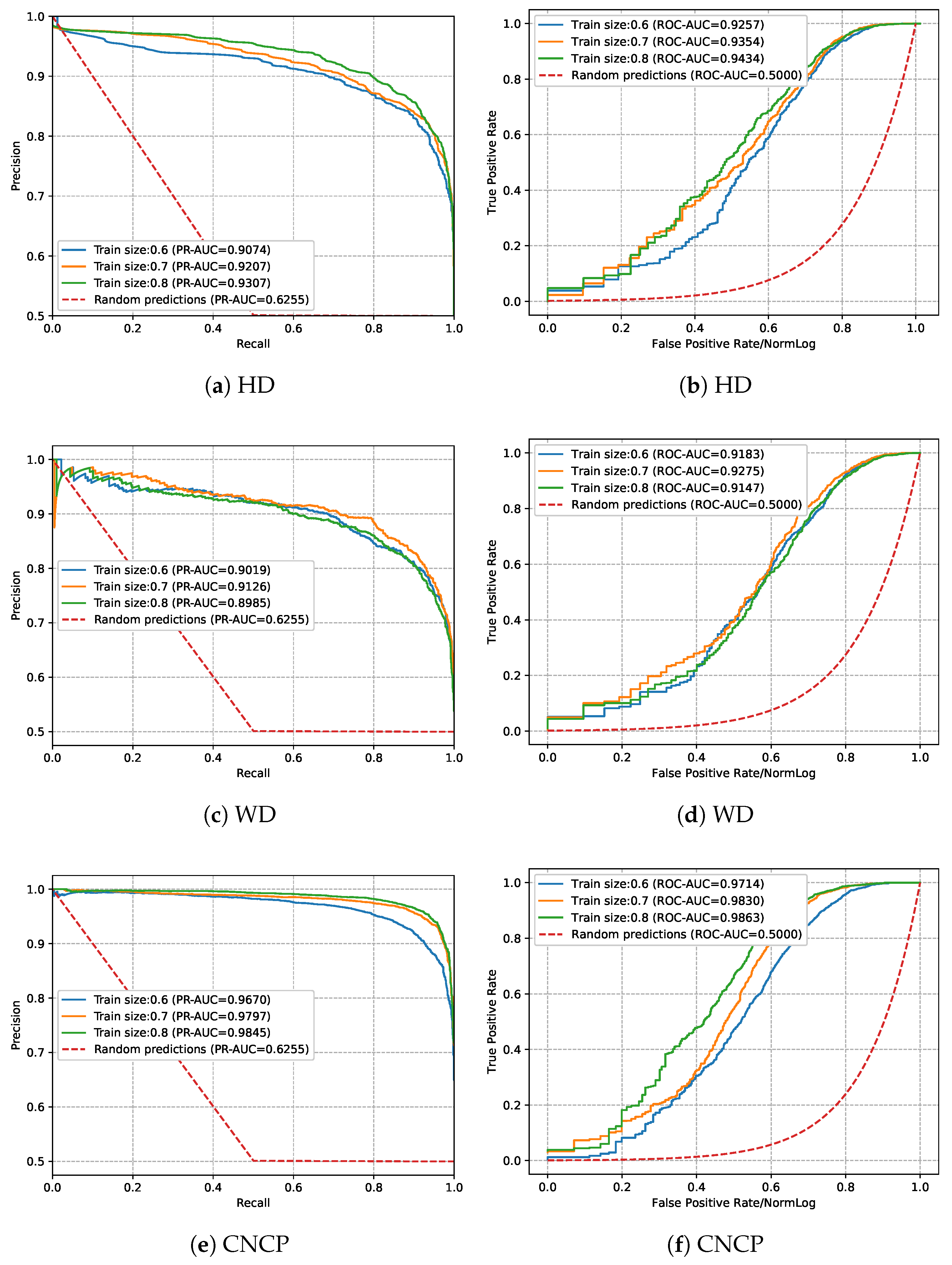
To better demonstrate the performance of the proposed method, in addition to the experiments in the previous section, we carried out extra experiments in which the ratio of the training data set to test data set were 6:4 and 7:3, respectively. The training processes are given in Figure 7, and the results are given in Table 6. We also give the area under the precision–recall curve (PR-AUC) and the area under the receiver operating characteristic curve (ROC-AUC) in Figure 8, as was carried out in [33], to show the relationship between precision and recall, as well as T P and F P .
Table 6 gives the test results, and Table 7 gives the sorted performance rank of nine methods, where HD-S is the result of HD with inputs 37 × 28 (e.g., inputs are four-week data), and CNCP-L is the result of the proposed method with input 148 × 7. These two methods were used to test the impact of the size of the input on the detection results. From Table 6 and Table 7, it can be seen that, in all tests, the SVM has the worst precision and random forest has the worst recall and F1-score. Meanwhile, the proposed method has the best precision, recall, and F1-score in all tests. Note that the performance of WD ranks second, indicating that the parallel network structure indeed improves the performance of the classification method; meanwhile, the performance of HD ranks third, indicating that, for time series data, the performance of the LSTM network is better than other single classifiers in this paper. Meanwhile, although the SVM has the worst precision, its recall ranks third, and its F1-score is in the middle of all nine methods. Therefore, when the performance requirement of the algorithm is not high and the complexity of the algorithm needs to be relatively low, the SVM may be a suitable algorithm. From Table 6, it can be seen that the result of HD-S is slightly lower than but similar to that of HD with the 148 × 7 matrix. The reason is that, for the LSTM method with the input of the 37 × 28 matrix, the input data can be considered as 37 × 28 vectors, meaning that its inputs are fewer but longer than the LSTM method with the 148 × 7 matrix. Although a longer input can benefit the LSTM method, fewer samples simultaneously reduce the performance of it. Meanwhile, we also tested the performance of the proposed CNCP-based method with inputs 148 × 7, which is labeled as CNCP-L. It can be seen that the performance of CNCP-L is lower than that of the CNCP. This may come from the fact that, for the CNN network, the 37 × 28 matrix has a smaller padding area than the 148 × 7 matrix during the convolution computing process, and can therefore yield better results.

3.3. Complexity Analysis

For deep neural networks, the computational complexity is usually presented by the total amount of floating-point operations per second (FLOPs) when processing a sample. The CNCP network proposed in this paper is mainly composed of a convolutional layer and fully connected layer. The FLOPs of a convolutional layer can be calculated by Equation (22):
C o n v = 2 × ( H K × W K × H I × W I ) × ( C I × C O )
The FLOPs of a fully connected layer can be calculated by Equation (23):
F C = 2 × C I × C O
where H K and W L are the height and width of the convolutional kernel, H I and W I are the height and width of the input data, and C I and C O are the number of input and output channels, respectively.
The CNCP network proposed in this paper adopts the structure of Conv-BN-Activation, the calculation of a BN layer is included in the calculation of the convolutional layer, and the FLOPs of the BN layer are negligible relative to the convolutional layer. Table 8 gives the computational complexity of the proposed CNCP network with 3 × 3 kernels, and Table 9 gives the computational complexity of the proposed CNCP network with different kernels.

4. Discussion

The advantage of the proposed method comes from the CNCP structure, which can capture features of electricity consumption time series at different scales. From Figure 2, Figure 3, Figure 4 and Figure 5, it can be seen that the normal electricity consumption time series has more significant periodic characteristics than the electricity theft time series. The algorithm proposed in this paper includes two branches, namely the convolution branch and the non-convolution branch. Using the data reconstructed based on the periodic characteristics of normal electricity consumption time series, if the periodic distribution of the electricity theft time series is significantly different from that of the normal electricity consumption time series, the convolution branch can realize effective theft detection. When the periodic distribution difference between theft data and normal data is not significant, the efficiency of the convolution branch is reduced. However, because the first layer of the non-convolution branch is the fully connected layer, the input data are globally mapped; that is, the classification is based on the global information of the data, which overcomes the problem of the low efficiency of the convolution branch so as to effectively improve the detection accuracy. For other time series analysis algorithms such as LSTM, it can be seen from the experiment section of this paper that the detection performance is lower than the proposed method. This is due to the fact that, for the LSTM model, according to the analysis in Section 2.3 and Section 2.4, the main difference between the electricity consumption of electricity theft users and that of normal users is their periodicity significance. LSTM can infer this periodic difference through extensive training. However, in this proposed method, the temporal data are first converted into 2D images based on the periodic feature of normal user electricity data, and electricity theft detection is carried out based on image classification. It can be considered that the proposed method utilizes the periodic prior of normal electricity data; therefore, the proposed method can achieve a better classification performance.
If a smart thief makes the features of their electricity consumption time series consistent with the normal time series, such as reducing the electricity consumption record to half of their normal electricity consumption by tampering with the smart meter, the algorithm proposed in this paper would not be applicable. In this situation, the problem of electricity theft detection can be regarded as a general binary classification problem, and some methods suitable for time series classification such as LSTM should be good choices. However, it is obvious that the classification methods that fully consider the data features would generally obtain a better accuracy.

5. Conclusions

Electricity theft detection is of great significance for ensuring the safety and stability of power systems, and it is a very challenging issue as there are many ways to steal electricity and electricity theft may not occur continuously. This paper analyzed the features of the load time series of normal residents and electricity thieves and proposed a novel CNCP-based method for electricity theft detection. Meanwhile, the influence and solution of the imbalance data were discussed. Extensive experiments prove the effectiveness of the proposed method. The core idea of the proposed method is that, compared with the load time series of electricity thieves, the normal residents’ load time series present more obvious periodicity. It is applicable in many practical electricity-stealing scenarios. Therefore, in the future research work, we will focus on this electricity theft scenario.

Author Contributions

Conceptualization, Y.W. and S.J.; methodology, Y.W.; software, Y.W.; validation, S.J. and M.C.; formal analysis, Y.W.; investigation, Y.W.; resources, S.J.; data curation, Y.W.; writing—original draft preparation, Y.W.; writing—review and editing, Y.W. and S.J.; visualization, Y.W; supervision, S.J.; project administration, S.J.; funding acquisition, S.J. All authors have read and agreed to the published version of the manuscript.

Funding

This work is supported by National Nature Science Foundation of China under Grant U22B20115.

Institutional Review Board Statement

Not applicable.

Informed Consent Statement

Not applicable.

Data Availability Statement

Data will be made available upon request.

Conflicts of Interest

The authors declare no conflict of interest.

References

  1. Ali, S.; Yongzhi, M.; Ali, W. Prevention and Detection of Electricity Theft of Distribution Network. Sustainability 2023, 15, 4868. [Google Scholar] [CrossRef]
  2. Kabir, B.; Qasim, U.; Javaid, N.; Aldegheishem, A.; Alrajeh, N.; Mohammed, E.A. Detecting Nontechnical Losses in Smart Meters Using a MLP-GRU Deep Model and Augmenting Data via Theft Attacks. Sustainability 2022, 14, 15001. [Google Scholar] [CrossRef]
  3. Oprea, S.V.; Bâra, A.; Puican, F.C.; Radu, I.C. Anomaly Detection with Machine Learning Algorithms and Big Data in Electricity Consumption. Sustainability 2021, 13, 10963. [Google Scholar] [CrossRef]
  4. Khattak, A.; Bukhsh, R.; Aslam, S.; Yafoz, A.; Alghushairy, O.; Alsini, R. A Hybrid Deep Learning-Based Model for Detection of Electricity Losses Using Big Data in Power Systems. Sustainability 2022, 14, 13627. [Google Scholar] [CrossRef]
  5. Khan, Z.A.; Adil, M.; Javaid, N.; Saqib, M.N.; Shafiq, M.; Choi, J.G. Electricity Theft Detection Using Supervised Learning Techniques on Smart Meter Data. Sustainability 2020, 12, 8023. [Google Scholar] [CrossRef]
  6. Xia, X.; Lin, J.; Xiao, Y.; Cui, J.; Peng, Y.; Ma, Y. A Control Chart based Detector for Small-amount Electricity Theft (SET) Attack in Smart Grids. IEEE Internet Things J. 2021, 9, 6745–6762. [Google Scholar] [CrossRef]
  7. Leite, J.B.; Mantovani, J.R.S. Detecting and Locating Non-Technical Losses in Modern Distribution Networks. IEEE Trans. Smart Grid 2018, 9, 1023–1032. [Google Scholar] [CrossRef] [Green Version]
  8. Cui, X.; Liu, S.; Lin, Z.; Ma, J.; Wen, F.; Ding, Y.; Yang, L.; Guo, W.; Feng, X. Two-Step Electricity Theft Detection Strategy Considering Economic Return Based on Convolutional Autoencoder and Improved Regression Algorithm. IEEE Trans. Power Syst. 2021, 37, 2346–2359. [Google Scholar] [CrossRef]
  9. Lin, Y.; Wang, J. Probabilistic Deep Autoencoder for Power System Measurement Outlier Detection and Reconstruction. IEEE Trans. Smart Grid 2020, 11, 1796–1798. [Google Scholar] [CrossRef]
  10. Zanetti, M.; Jamhour, E.; Pellenz, M.; Penna, M.; Zambenedetti, V.; Chueiri, I. A Tunable Fraud Detection System for Advanced Metering Infrastructure Using Short-Lived Patterns. IEEE Trans. Smart Grid 2019, 10, 830–840. [Google Scholar] [CrossRef]
  11. Peng, Y.; Yang, Y.; Xu, Y.; Xue, Y.; Song, R.; Kang, J.; Zhao, H. Electricity Theft Detection in AMI Based on Clustering and Local Outlier Factor. IEEE Access 2021, 9, 107250–107259. [Google Scholar] [CrossRef]
  12. Biswas, P.P.; Cai, H.; Zhou, B.; Chen, B.; Mashima, D.; Zheng, V.W. Electricity Theft Pinpointing Through Correlation Analysis of Master and Individual Meter Readings. IEEE Trans. Smart Grid 2020, 11, 3031–3042. [Google Scholar] [CrossRef]
  13. Jokar, P.; Arianpoo, N.; Leung, V.C.M. Electricity Theft Detection in AMI Using Customers’ Consumption Patterns. IEEE Trans. Smart Grid 2016, 7, 216–226. [Google Scholar] [CrossRef]
  14. Song, C.; Sun, Y.; Han, G.; Rodrigues, J.J. Intrusion detection based on hybrid classifiers for smart grid. Comput. Electr. Eng. 2021, 93, 107212. [Google Scholar] [CrossRef]
  15. Hu, T.; Guo, Q.; Shen, X.; Sun, H.; Wu, R.; Xi, H. Utilizing Unlabeled Data to Detect Electricity Fraud in AMI: A Semisupervised Deep Learning Approach. IEEE Trans. Neural Networks Learn. Syst. 2019, 30, 3287–3299. [Google Scholar] [CrossRef]
  16. Messinis, G.M.; Rigas, A.E.; Hatziargyriou, N.D. A Hybrid Method for Non-Technical Loss Detection in Smart Distribution Grids. IEEE Trans. Smart Grid 2019, 10, 6080–6091. [Google Scholar] [CrossRef]
  17. Buzau, M.M.; Tejedor-Aguilera, J.; Cruz-Romero, P.; Gómez-Expósito, A. Detection of Non-Technical Losses Using Smart Meter Data and Supervised Learning. IEEE Trans. Smart Grid 2019, 10, 2661–2670. [Google Scholar] [CrossRef]
  18. Avila, N.F.; Figueroa, G.; Chu, C.C. NTL Detection in Electric Distribution Systems Using the Maximal Overlap Discrete Wavelet-Packet Transform and Random Undersampling Boosting. IEEE Trans. Power Syst. 2018, 33, 7171–7180. [Google Scholar] [CrossRef]
  19. Jindal, A.; Dua, A.; Kaur, K.; Singh, M.; Kumar, N.; Mishra, S. Decision Tree and SVM-Based Data Analytics for Theft Detection in Smart Grid. IEEE Trans. Ind. Inform. 2016, 12, 1005–1016. [Google Scholar] [CrossRef]
  20. Song, C.; Xu, W.; Han, G.; Zeng, P.; Wang, Z.; Yu, S. A Cloud Edge Collaborative Intelligence Method of Insulator String Defect Detection for Power IIoT. IEEE Internet Things J. 2021, 8, 7510–7520. [Google Scholar] [CrossRef]
  21. Hu, T.; Guo, Q.; Sun, H.; Huang, T.E.; Lan, J. Nontechnical Losses Detection Through Coordinated BiWGAN and SVDD. IEEE Trans. Neural Netw. Learn. Syst. 2021, 32, 1866–1880. [Google Scholar] [CrossRef] [PubMed]
  22. Aldegheishem, A.; Anwar, M.; Javaid, N.; Alrajeh, N.; Shafiq, M.; Ahmed, H. Towards Sustainable Energy Efficiency With Intelligent Electricity Theft Detection in Smart Grids Emphasising Enhanced Neural Networks. IEEE Access 2021, 9, 25036–25061. [Google Scholar] [CrossRef]
  23. Punmiya, R.; Choe, S. Energy Theft Detection Using Gradient Boosting Theft Detector With Feature Engineering-Based Preprocessing. IEEE Trans. Smart Grid 2019, 10, 2326–2329. [Google Scholar] [CrossRef]
  24. Yan, Z.; Wen, H. Electricity Theft Detection Base on Extreme Gradient Boosting in AMI. IEEE Trans. Instrum. Meas. 2021, 70, 1–9. [Google Scholar] [CrossRef]
  25. Bian, J.; Wang, L.; Scherer, R.; Woźniak, M.; Zhang, P.; Wei, W. Abnormal Detection of Electricity Consumption of User Based on Particle Swarm Optimization and Long Short Term Memory With the Attention Mechanism. IEEE Access 2021, 9, 47252–47265. [Google Scholar] [CrossRef]
  26. Takiddin, A.; Ismail, M.; Nabil, M.; Mahmoud, M.M.E.A.; Serpedin, E. Detecting Electricity Theft Cyber-Attacks in AMI Networks Using Deep Vector Embeddings. IEEE Syst. J. 2021, 15, 4189–4198. [Google Scholar] [CrossRef]
  27. Massaferro, P.; Martino, J.M.D.; Fernández, A. Fraud Detection in Electric Power Distribution: An Approach That Maximizes the Economic Return. IEEE Trans. Power Syst. 2020, 35, 703–710. [Google Scholar] [CrossRef]
  28. Gao, Y.; Foggo, B.; Yu, N. A Physically Inspired Data-Driven Model for Electricity Theft Detection With Smart Meter Data. IEEE Trans. Ind. Inform. 2019, 15, 5076–5088. [Google Scholar] [CrossRef]
  29. Ramos, C.C.O.; Rodrigues, D.; de Souza, A.N.; Papa, J.P. On the Study of Commercial Losses in Brazil: A Binary Black Hole Algorithm for Theft Characterization. IEEE Trans. Smart Grid 2018, 9, 676–683. [Google Scholar] [CrossRef] [Green Version]
  30. Lin, G.; Feng, X.; Guo, W.; Cui, X.; Liu, S.; Jin, W.; Lin, Z.; Ding, Y. Electricity Theft Detection Based on Stacked Autoencoder and the Undersampling and Resampling Based Random Forest Algorithm. IEEE Access 2021, 9, 124044–124058. [Google Scholar] [CrossRef]
  31. Takiddin, A.; Ismail, M.; Zafar, U.; Serpedin, E. Robust Electricity Theft Detection Against Data Poisoning Attacks in Smart Grids. IEEE Trans. Smart Grid 2021, 12, 2675–2684. [Google Scholar] [CrossRef]
  32. Aslam, Z.; Ahmed, F.; Almogren, A.; Shafiq, M.; Zuair, M.; Javaid, N. An Attention Guided Semi-Supervised Learning Mechanism to Detect Electricity Frauds in the Distribution Systems. IEEE Access 2020, 8, 221767–221782. [Google Scholar] [CrossRef]
  33. Buzau, M.M.; Tejedor-Aguilera, J.; Cruz-Romero, P.; Gómez-Expósito, A. Hybrid Deep Neural Networks for Detection of Non-Technical Losses in Electricity Smart Meters. IEEE Trans. Power Syst. 2020, 35, 1254–1263. [Google Scholar] [CrossRef]
  34. Zheng, K.; Chen, Q.; Wang, Y.; Kang, C.; Xia, Q. A Novel Combined Data-Driven Approach for Electricity Theft Detection. IEEE Trans. Ind. Inform. 2019, 15, 1809–1819. [Google Scholar] [CrossRef]
  35. Zheng, Z.; Yang, Y.; Niu, X.; Dai, H.; Zhou, Y. Wide and Deep Convolutional Neural Networks for Electricity-Theft Detection to Secure Smart Grids. IEEE Trans. Ind. Inform. 2018, 14, 1606–1615. [Google Scholar] [CrossRef]
  36. Song, C.; Jing, W.; Zeng, P.; Yu, H.; Rosenberg, C. Energy consumption analysis of residential swimming pools for peak load shaving. Appl. Energy 2018, 220, 176–191. [Google Scholar] [CrossRef]
  37. Song, C.; Jing, W.; Zeng, P.; Rosenberg, C. An analysis on the energy consumption of circulating pumps of residential swimming pools for peak load management. Appl. Energy 2017, 195, 1–12. [Google Scholar] [CrossRef]
  38. SGCC. Analysis on Abnormal Behavior of Electricity Customers. Available online: https://www.datafountain.cn/competitions/241 (accessed on 4 April 2022).
  39. Simonyan, K.; Zisserman, A. Very Deep Convolutional Networks for Large-Scale Image Recognition. In Proceedings of the International Conference on Learning Representations, San Diego, CA, USA, 7–9 May 2015. [Google Scholar]
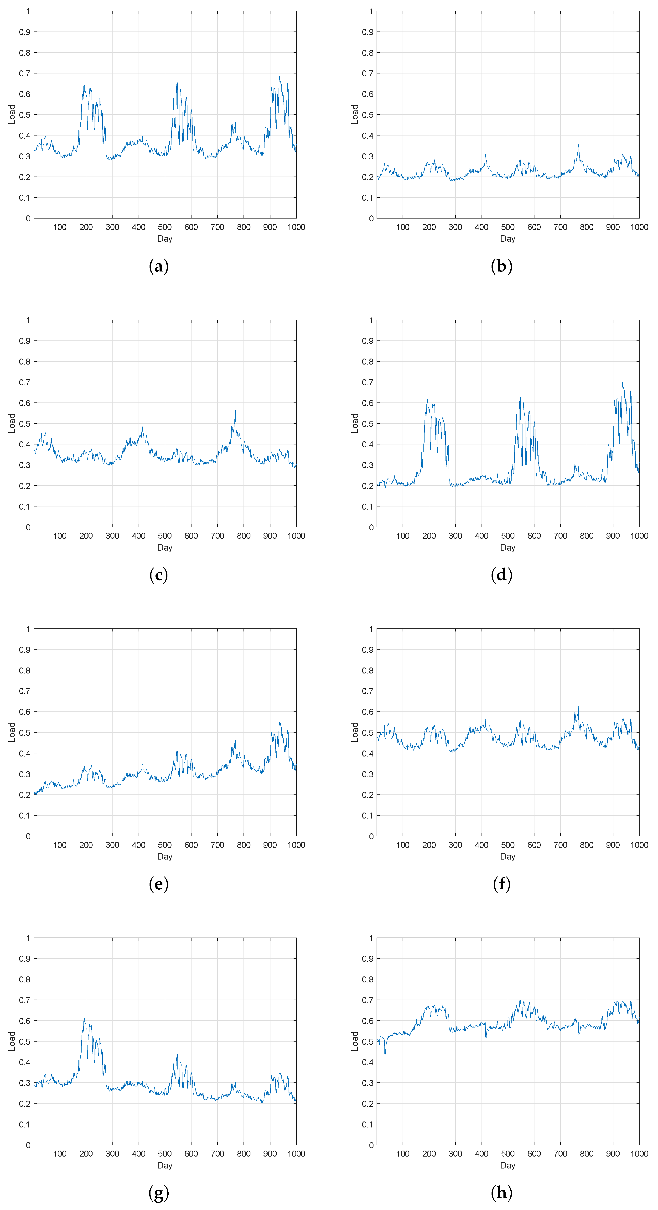
Figure 1. (ah) Load main patterns of normal residents after clustering.
Sustainability 15 10127 g001
Figure 2. (ah) Load main patterns of electricity thieves after clustering.
Sustainability 15 10127 g002
Figure 3. (ah) Images of loads of normal residents.
Sustainability 15 10127 g003
Figure 4. (ah) Images of loads of electricity thieves.
Sustainability 15 10127 g004
Figure 5. The overall structure of the proposed detection method.
Sustainability 15 10127 g005
Figure 6. An example structure of the proposed method based on C1-N1.
Sustainability 15 10127 g006
Figure 7. The training processes.
Sustainability 15 10127 g007
Figure 8. Comparisons with other methods.
Sustainability 15 10127 g008
Table 1. Short-period-comparison-based electricity theft detection methods.
Refs.AlgorithmsCore IdeasData SourceNormal DataTheft Data
 [6]Control chartThe mean and variance of short-period normal data and short-period theft data are obviously different.SimulatedSimulatedSimulated
 [7]Control chartThe mean and variance of short-period normal data and short-period theft data are obviously different.SimulatedSimulatedSimulated
 [8]Convolutional autoencoderThe error of reconstructed theft data would be large using the autoencoder trained by short-period normal data.IEEE 33-bus test systemSimulatedSimulated
 [9]Probabilistic deep autoencoderThe error of reconstructed theft data would be large using the autoencoder trained by short-period normal data.-SimulatedSimulated
 [10]FCM, K-means and SOMShort-period normal data and short-period theft data will appear in different clusters.Irish Smart Energy Trail datasetRealSimulated
 [11]Clustering and local outlier factorShort-period normal data and short-period theft data will appear in different clusters.-RealSimulated
 [12]Correlation analysisThe correlation between short-period normal data and short-period theft data would be significantly low.Irish Smart Energy Trail datasetRealSimulated
 [13]Consumption patternThe specific theft mode will lead to a special abnormal state of data.Irish Smart Energy Trail datasetRealSimulated
Table 2. Two-stage whole-period-classification electricity theft detection methods.
Refs.AlgorithmsData SourceNormal DataTheft Data
 [15]Seven feature extraction networks + one discrimination networkIrish Smart Energy Trail datasetRealSimulated
 [16]Breakout detection + SVMIrish Smart Energy Trail datasetRealSimulated
 [17]Six feature extraction methods + XGBoostA private data set from Endesa in SpainRealReal
 [18]Discrete wavelet transform + random undersampling boosting-RealReal
 [19]Decision tree + SVMA private data set from USARealSimulated
Table 3. One-stage whole-period-classification electricity theft detection methods.
Refs.AlgorithmsData SourceNormal DataTheft Data
 [21]Support vector descriptionIrish Smart Energy Trail datasetRealSimulated
[22]AlexNet + LightGBMThe State Grid
Corporation of China
RealReal
GoogLeNet + AdaBoost
 [23]XGBoost, CatBoost, LightGBMIrish Smart Energy Trail datasetRealSimulated
 [24]XGBoostIrish Smart Energy Trail datasetRealSimulated
 [25]LSTMA private data set from the University of MassachusettsRealSimulated
[26]Deep vector embeddingsIrish Smart Energy Trail datasetRealSimulated
The State Grid Corporation of ChinaRealReal
[27]Bayesian risk
framework
A private data set from MontevideoRealSimulated
A private data set from MontevideoRealReal
 [28]Linear regressionA private data set from Southern California Edison (SCE) service territoryRealSimulated
 [29]Black hole algorithmTwo private datasets from a Brazilian electric utilityRealReal
[30]Stacked autoencoder
+ random forest
Irish Smart Energy Trail datasetRealSimulated
A private data set from ChinaRealReal
 [31]Deep autoencoder + feed forward neural networksIrish Smart Energy Trail datasetRealSimulated
[32]Relational autoencoder
+ TripleGAN
Irish Smart Energy Trail datasetRealSimulated
A private data set from MontevideoRealReal
 [33]LSTM + MLPA private data set from Endesa in SpainRealReal
 [34]The maximum information coefficient + fast search and find of density peaksIrish Smart Energy Trail datasetRealSimulated
 [35]BP + CNNThe State Grid Corporation of ChinaRealReal
Our MethodConvolution + non-convolution deep networkThe State Grid Corporation of ChinaRealReal
Table 4. Backbone networks adopted in the proposed method.
BranchCodeStructure
Convolution branch [39]C1VGG11
C2VGG13
C3VGG16
Non-convolution branchN1fc64-relu-fc2-softmax
N2fc128-relu-fc64-relu-fc2-softmax
N3fc256-relu-fc128-relu-fc64-relu-fc2-softmax
N4fc512-relu-fc256-relu-fc128-relu-fc64-relu-fc2-softmax
N5fc1024-relu-fc512-relu-fc256-relu-fc128-relu-fc64-relu-fc2-softmax
Table 5. Experiment results on different backbone structures in the proposed method.
Structure TPFPFNTNPrecisionRecallF1Score
Convolution
branch
C10.79970.17760.07270.90450.81830.91670.8647
C20.8530.12420.02760.94970.87290.96870.9183
C30.75040.22680.1220.85530.76790.86020.8114
Non-
convolution
branch
N10.8510.12630.08940.88780.87080.90490.8875
N20.84130.13590.04370.93360.86090.95060.9036
N30.85940.11790.04250.93470.87940.95290.9146
N40.83280.14440.05120.9260.85220.94210.8949
N50.67530.3020.28570.69160.69100.70270.6968
CNCP
network
C1+N10.86560.11170.07710.90010.88570.91820.9017
C1+N20.93180.04540.03050.96680.95350.96830.9609
C1+N30.92020.05710.01910.96820.94160.97970.9602
C2+N10.86340.11380.07520.9020.88350.91990.9013
C2+N20.93020.04750.01550.96170.95140.98360.9672
C2(3)+N30.92310.04780.01220.9750.95080.98700.9685
C2(5)+N30.92220.05910.01310.97380.93980.98600.9623
C2(7)+N30.91840.08520.01490.96150.91510.98400.9483
C3+N10.87060.10660.06350.91370.89090.93200.9110
C3+N20.91580.06150.01430.9630.93710.98460.9603
C3+N30.90860.06860.01220.9650.92980.98680.9574
Table 6. Comparisons with other methods.
Training = 60%Training = 70%Training = 80%
PrecisionRecallF1-ScorePrecisionRecallF1-ScorePrecisionRecallF1-Score
SVM0.59490.85450.70150.59670.85590.70320.59840.85700.7047
LR0.73910.63120.68090.74430.63670.68630.74570.63620.6866
RF0.84610.40400.54690.86670.37350.52200.87470.35220.5022
XGB0.87120.48920.62660.87870.48730.62690.88370.46920.6130
HD0.90130.68160.77620.94520.59370.72930.91090.68080.7792
HD-S0.90100.68090.77560.94460.59280.72840.91020.68140.7794
WD0.83270.91580.87230.83780.90410.86970.82800.89820.8617
CNCP-L0.91210.92480.91840.93570.93220.93390.94720.98210.9643
CNCP0.91250.92530.91890.93920.93850.93880.95080.9870.9685
Table 7. Performance ranks.
Training = 60%Training = 70%Training = 80%
PrecisionRecallF1-ScorePrecisionRecallF1-ScorePrecisionRecallF1-Score
1CNCPCNCPCNCPCNCPCNCPCNCPCNCPCNCPCNCP
2CNCP-LCNCP-LCNCP-LCNCP-LCNCP-LCNCP-LCNCP-LCNCP-LCNCP-L
3HDWDWDHDWDWDHDWDWD
4HD-SSVMHDHD-SSVMHDHD-SSVMHD
5XGBHDHD-SXGBHDHD-SXGBHDHD-S
6RFHD-SSVMRFHD-SSVMRFHD-SSVM
7WDLRXGBWDLRLRWDLRLR
8LRXGBLRLRXGBXGBLRXGBXGB
9SVMRFRFSVMRFRFSVMRFRF
Table 8. The computational complexity of each layer of the proposed CNCP network.
Convolution BranchNon-Convolution Branch
LayerFLOPsLayerFLOPs
Conv_12 × (3 × 3 × 37 × 28) × (1 × 64)FC256(37 × 28) × 256
Conv_22 × (3 × 3 × 37 × 28) × (64 × 64)FC128256 × 128
Max_pool37 × 28 × 64FC64128 × 64
Conv_32 × (3 × 3 × 19 × 14) × (64 × 128)
Conv_42 × (3 × 3 × 19 × 14) × (128 × 128)
Max_pool19 × 14 × 128
Conv_52 × (3 × 3 × 10 × 7) × (128 × 256)
Conv_62 × (3 × 3 × 10 × 7) × (256 × 256)
Conv_72 × (3 × 3 × 10 × 7) × (256 × 256)
Gmpool256 × 10 × 7
FC60256 × 60
Table 9. The computational complexity of the proposed CNCP network with different kernels.
Size of the KernelFLOPs
3 × 34.02 × 10 8
5 × 51.116 × 10 9
7 × 72.187 × 10 9
Disclaimer/Publisher’s Note: The statements, opinions and data contained in all publications are solely those of the individual author(s) and contributor(s) and not of MDPI and/or the editor(s). MDPI and/or the editor(s) disclaim responsibility for any injury to people or property resulting from any ideas, methods, instructions or products referred to in the content.