Article

Evolution of Landscape Ecological Risk and Identification of Critical Areas in the Yellow River Source Area Based on LUCC

1
Department of Geological Engineering, Qinghai University, Xining 810016, China
2
Provincial Key Laboratory of Cenozoic Resources and Environment on the Northern Rim of the Qinghai–Tibet Plateau, Qinghai University, Xining 810016, China
*
Author to whom correspondence should be addressed.
Sustainability 2023, 15(12), 9749; https://doi.org/10.3390/su15129749
Submission received: 29 April 2023 / Revised: 15 June 2023 / Accepted: 16 June 2023 / Published: 19 June 2023
(This article belongs to the Special Issue Bringing Ecosystem Services into Decision-Making)

Abstract

:
A reasonable evaluation of the ecological risk status of the landscape in the Yellow River source area is of practical significance for optimizing the regional landscape pattern and maintaining ecosystem function. To explore the regional heterogeneity of ecological risk in the watershed landscape, a landscape ecological risk evaluation model is constructed to evaluate the ecological risk status of the watershed for 20 years, and correlation analysis is used to further reveal the characteristics of the relationship between ecological risk and land use. The results show that the rapid expansion of urbanization and the increasing intensity of land development and use has caused significant changes in the Yellow River source area ecological environment and various land use types. The area of grassland decreased the most, by a total of 6160.04 km2, while the area of unused land increased the most, by a total of 2930.27 km2. A total of 12,453.11 km2 of land in the Yellow River source area was transformed, accounting for 9.52% of the total area. The most significant area of grassland was transferred out, accounting for 49.47% of the transferred area. During the study period, the proportion of area in the low-risk zone decreased from 54.75% to 36.35%, the proportion of area in the medium-low-risk zone increased from 21.75% to 31.74%, and the proportion of area in the medium-high-risk and high-risk zones increased from 10.63% to 14.38%. The high-risk areas are mainly located in areas with fragmented landscapes and are vulnerable to human activities. The mean ecological risk values in the study area show an increasing trend, and the spatial distribution shows a hierarchical distribution of “lower around the center and higher in the center”. The global Moran’s I index is higher than 0.68, which indicates that the ecological risk values have a significant positive correlation in space, the area of cold spots of ecological risk varies significantly, and the spatial pattern fluctuates frequently, while the spatial distribution of hot spots is relatively stable. Therefore, the landscape ecological risk in the Yellow River source area is rising, but the different risk levels and their spatial aggregation patterns and cold and hot spot areas continue to transform, which requires continuous planning of the landscape pattern to enhance the safety and stability of the regional ecosystem.

1. Introduction

Ecological risk refers to the degree of risk faced by an ecosystem in response to natural or human interference [1]. When the introduction of sustainable development was proposed in 1972, the international community began to pay attention to ecological risk assessment [2]. In 1992, the U.S. Environmental Protection Agency acknowledged the concept of ecological risk assessment and established a relevant assessment framework, which has since been continuously developed and improved [3]. Ecological risk assessment research has been influenced by the geographic research of ecologization and the macrocosm of ecological research and has rapidly expanded from the ecosystem scale to the landscape scale. Its evaluation object has been expanded from a single type of ecosystem to a spatial mosaic of multiple ecosystems [4]. Landscape ecological risk assessment refers to the process that starts with the mosaic of landscape elements, landscape pattern evolution, and landscape ecological processes, by analyzing the response of ecosystems to intrinsic risk sources and external disturbances. It is an important component in ecological safety assessment, which can reflect the spatial distribution of regional risks in an integrated manner and clarify the degree of disturbance to ecosystem structure and function caused by changes in land use types [4]. The landscape consists of heterogeneous elements whose heterogeneity is closely related to the disturbance capacity, recovery capability, stability, and diversity of the ecosystem. Due to the high heterogeneity of the landscape, the process of changing its overall structure and dynamics is slow. However, the spatial components that make up the landscape can change at different rates and intensities when they are disturbed. Therefore, ecological risk evaluation can measure the key elements of risk receptor range and hazard status through the slow variation of the landscape [5,6]. In general, compared with a single evaluation index and a single evaluation method, ecological risk assessment can evaluate the security and stability of ecosystems from a comprehensive and global perspective, and can more comprehensively reflect the complexity and diversity of ecosystems [7,8]. Meanwhile, the study of land use pattern status in the ecological restoration process from the perspective of landscape ecology can accurately represent the heterogeneity within regions and the correlation between regions [9].
Currently, scholars mainly study and assess landscape pattern functions and regional ecological security [10]. The main assessment methods include the Landscape Index Method and the Relative Risk Model [11]. The Landscape Index Method constructs ecological risk indices and develops assessment models by selecting different types of landscape pattern indices [12]. Based on remote sensing images, the land use transfer matrix, and the Ecological Risk Index (ERI), and combined with GIS spatial analysis and Fragstats 4.2.1, the models are widely used in contemporary research to assess regional ecological risk from multiple perspectives, including macro-regional, “production-life-ecological space”, and “natural-social-landscape pattern”, studying the areas of land type, watershed, and urban landscape [13,14,15,16]. Scholars have thoroughly explored the influencing factors, driving mechanisms, and spatial and temporal differentiation of ecological risks in landscapes and related ecological safety patterns. These studies have provided the theoretical foundation for the mechanisms of maintaining the functional stability and integrity of ecosystems [17,18,19,20]. However, current ecological risk evaluation studies still take administrative units as evaluation units and ignore the grid-scale (vector) ecological risk evaluation that could better reflect the spatial heterogeneity of the results. In recent years, due to disturbance by natural or human factors such as population growth, irrationalization of industrial structure, unbalanced regional development, and continuous expansion of construction land, the structure and function of the ecosystem have changed, ecological and environmental pressures have increased, and ecological and environmental effects have fluctuated significantly, leading to frequent problems of ecosystem degradation, prominent ecological risk problems, and significant spatial and temporal differences [21]. Since 1999, China has implemented ecological restoration projects such as reforestation of barren mountains and the return of cultivated land to forest or grass, and the vegetation restoration of these projects has played a significant role in maintaining ecological security and controlling sustainable land use in the source area of the Yellow River, ensuring that the regional landscape pattern; soil erosion; land use layout; and structure of agriculture, forestry, and animal husbandry is scientifically improved, and the quality of the ecological environment has been effectively enhanced [22,23,24,25]. Therefore, studying the land use pattern situation in the ecological restoration process from the perspective of landscape ecology can accurately indicate the heterogeneity within the region and the inter-regional correlation.
At present, studies on landscape ecological risks are mostly focused on larger river basins or coastal economic development zones where human activities are intense. However, the landscape risk status of natural areas with more fragile ecology, such as grasslands, has yet to be further investigated. The high-altitude topography of the Yellow River source area leads to its unique climatic characteristics, human activities, and spatial pattern of ecological landscape. With the rapid development of the regional economy and global climate change, land use types are changing drastically, with strong spatial heterogeneity in the regional ecological risk. Therefore, the evaluation of landscape ecological risk in this region has strong regional characteristics and typicality. This study takes the ecologically fragile Yellow River source area as the research object. Referring to land use data in 2000, 2010, and 2020, Fragstats 4.2 software is used to calculate the landscape grid index and constructed an ecological risk evaluation model by combining the landscape fragility index. The hierarchy and spatial and temporal divergence patterns of ecological risks are analyzed by grid scale; in addition, the response relationship between land use intensity and ecological risks is explored, along with the spatial and temporal aggregation characteristics of ecological risks and the evolution pattern of cold hot spots. The study provides theoretical support for erosion control, biodiversity cultivation, vegetation landscape continuity, and rational layout in the Yellow River source area. From a spatial and temporal perspective, this study analyzes in detail land use changes, landscape ecological risk changes, land use and ecological risk linkages, and the spatial distribution changes of local ecological risk in the Yellow River source area. The analysis provides theoretical support for erosion control, biodiversity cultivation, the continuity of vegetation landscape, and reasonable layout in the Yellow River source area.

2. Materials and Methods

2.1. Study Area

The Tibet Plateau is an important strategic place of water resources and an ecological security barrier in China. The Yellow River source area, located in the northeast end of the Tibet Plateau, 32.5°~36.5° N, 95°~103.5° E, across the three provinces of Qinghai, Gansu, and Sichuan, is the largest flow-producing area of the Yellow River Basin and is an extremely important recharge area of freshwater resources and ecological function area in China. It has a total area of 130,000 km2, and the terrain is high in the west and low in the east. The average elevation is 4500 m, the highest point is 6265 m above sea level (located in Animaqing Mountain), and the lowest point is 2418 m above sea level (located near Longyangxia Reservoir). The Yellow River source area is mainly a plateau continental climate with dry and wet seasons, long sunshine hours, low vegetation cover, and precipitation decreasing from east to west. The land use type is mainly grass, and the rest of it is unused land. It has Zaling Lake and Eling Lake in the West. The industrial structure in the Yellow River source area is simplex; animal husbandry is the main industry. In recent years, global warming has become increasingly significant, where the permafrost is rapidly melting, and the watershed water has increased. These phenomena result in soil erosion, land degradation, ecosystem damage, etc.

2.2. Data Sources

This paper uses land use/land cover data for 2000, 2010, and 2020, with datasets from GlobeLand30 (http://www.globallandcover.com, accessed on 10 January 2023). The classified images used for data development are mainly 30-m multispectral images, including the US Land Resources Satellite (Landsat) TM5, ETM+, OLI multispectral images, and Chinese Environmental Disaster Reduction Satellite (HJ-1) multispectral images, and the 2020 version of the data also used 16-m resolution High-Fraction-1 (GF-1) multispectral images, with a spatial resolution of 30 m, an overall accuracy of 85.72%, and a Kappa coefficient of 0.82 [26]. According to the ecosystem environment and land resource use attributes in the study area, and concerning the Standard for Current Land Use Classification (GB/T 21010-2017) [27], the land use types were classified as farmland, woodland, grassland, wetland, water, construction land, and unused land (Table 1).

2.3. Land Use Transfer Matrix Model

The land use transfer matrix is a two-dimensional matrix constructed based on the relationship between land use changes in the study area at different times [28]. It can reflect in detail the dynamic information of the interconversion of the area of various land types in the study area at the beginning of the study period and at the end of the study period, and can not only indicate the area data of various land types in the study area at a certain point of time but also reveal the information of the area transfer out of various land types at the beginning of the period and the area transfer in of various land types at the end of the period [29]. In this study, the land use change in the Yellow River source area from 2000 to 2020 was made into a Sankey diagram to show the land use change. The land use transfer matrix equation is as follows:
A i j = A 11 A 12   A 1 n A 21 A n 1 A 22 A n 2 A 2 n A n n
In the formula, A i j represents the state of ecological land from the early to the end of the study and n represents the number of ecological land types.

2.4. Division of Evaluation Unit

In order to spatially express the regional heterogeneity of ecological risk in the landscape, the study area was divided into ecological risk evaluation units. Referring to the relevant standard of national grid GIS, Geographic Grid (GB12409-2009) [30], and some scholars’ research, it is appropriate to use 2~5 times the average patch area for the grid [31,32], and according to the area of the study area, a square grid of 10 km × 10 km was selected to divide the study area in this paper, and a total of 1785 ecological risk cells were obtained (Figure 1). In each cell, the Ecological Risk Index (ERI) was calculated, and the results were assigned to the center point of the evaluation cell.

2.5. Landscape Ecological Risk Index Evaluation

In this paper, the landscape ecological risk index of the Yellow River source area was constructed using the landscape disturbance index and the landscape fragility index from the proportion of landscape components in different years, respectively. This index reflects the relationship between landscape pattern and ecological risk in the Yellow River source area based on land use [33,34,35], which is calculated as follows:
E R I k = i = 1 N A k i A k × D i × V i
In the formula, k is the risk plot, i is the landscape type, N is the number of landscape types, A k i is the area of landscape types i in k risk plots, A k is the area of the first risk plot, D i is the landscape disturbance index, and V i is the landscape fragility index. The higher the E R I value, the higher the ecological risk. The specific formula and explanation are shown in Table 2.

2.6. Regional Ecological Risk Analysis

Based on the calculation of ERI indices of each risk assessment unit, the regional ecological risk analysis was achieved using geostatistical methods and GIS technology. The ERI were assigned to the center points of the risk assessment units, and the ERI spatial distribution map of the whole study area was obtained by ordinary kriging interpolation. The natural breakpoint method was used to classify the ecological risk of the landscape into five levels, namely, high-risk area (ERI > 0.03826), medium-high-risk area (0.03259 < ERI ≤ 0.03826), medium-risk area (0.02818 < ERI ≤ 0.03259), medium-low-risk area (0.02472 < ERI ≤ 0.02818), and low-risk area (≤0.02472).

2.7. Exploratory Spatial Data Analysis

In this paper, we adopt an exploratory spatial data analysis method, based on the distribution pattern of spatial data, aiming to discover the spatial aggregation pattern and association pattern of data in the study area to reveal the spatial heterogeneity characteristics of data [36]. Specifically, two methods, local spatial auto-correlation analysis and local hotspot analysis, are used to explore the spatial aggregation and correlation of ecological risks in the study area. In this paper, Moran’s I, LISA, and Getis-Ord G i * were used to characterize the spatial relationships of ecological risks in the study area [37].
Moran’s I statistic, as a spatial auto-correlation statistic, is used to reflect the degree of similarity between the genus values of spatially adjacent or similar units. The formula is:
I = n i j ω i j ( Y i Y ¯ ) ( Y j Y ¯ ) ( i j ω i j ) i ( Y i Y ¯ ) 2
In the formula, Y i , Y j is the value of the variable in the adjacent paired spatial units, ω i j is the spatial weight matrix, and Y ¯ is the mean of the attribute values. I takes values between [−1, 1]. When I > 0, it indicates that the observations of the study unit tend to be spatially aggregated and spatially positively correlated, when I < 0, it indicates a discrete spatial distribution and spatially negatively correlated, and when I = 0, it indicates spatially uncorrelated.
The LISA index, also known as the local Moran’s I, can reflect the degree of difference and significance between a region and its neighboring regions. The formula is:
I i = Y i Y ¯ S 2 j i n ω i j ( Y j Y ¯ )
S 2 = 1 n ( Y i Y ¯ ) 2
In the formula, n is the number of samples, i.e., the number of study units, and S 2 is the variance of the statistic. When I i > 0, it means that a region with high (low) observations is surrounded by a region with high (low) observations, i.e., “high–high (“low–low”) aggregation, when I i < 0, it means that a region with high (low) observations is surrounded by a region with low (low) observations, i.e., “high–low” (“low–high”) aggregation, and when I i = 0, it means that the observed region is not associated with the adjacent region, i.e., not significant.
The local spatial association index (Getis-Ord G i * ) is used to study the local spatial aggregation patterns and locations of high- and low-value elements. The formula is:
G i * = j = 1 n ω i , j x j X ¯ j = 1 n ω i , j S n j = 1 n ω i , j 2 j = 1 n ω i , j 2 n 1
X ¯ = j = 1 n x j n
S = j = 1 n x j n X ¯ 2
In the formula, x j is the attribute value of element j , ω i , j is the spatial weight between elements i and j , and n is the total number of elements. To simplify it, it is necessary to normalize G i * : Z ( G i * ) = G i * E ( G i * ) / V a r ( G i * ) . E ( G i * )   a n d   V a r ( G i * ) are taken as the mathematical expectation of G i * as well as the number of variances, respectively. When Z ( G i * ) > 0 and the test is significant, it indicates that the ecological safety index around the region within the study area is relatively high, which is a hot spot area within the region; when Z ( G i * ) < 0 and the test is significant, it indicates that the ecological safety index around the region i within the study area is relatively low and is a cold spot area within the region.

2.8. Pearson Correlation Analysis

The Pearson correlation coefficient can reflect the linear relationship between two variables, X and Y. This paper studies the degree of correlation between land use intensity and ecological risk index, which facilitates the understanding of the link between land use change and ecological risk [38]. The formula is:
r = i = 1 n ( X i X ¯ ) ( Y i Y ¯ ) i = 1 n ( X i X ¯ ) 2 i = 1 n ( Y i Y ¯ ) 2
In the formula, the range of values of r is [−1, 1], when r = 0, X, Y are independent. When 0 < r 1 , r is a positive correlation. When 1 r < 0 , r is a negative correlation. The more r is closer to 1, the stronger is the correlation between X and Y.

3. Results and Analysis

3.1. Land Use Changes

The spatial distribution and area changes of land use in the Yellow River source area from 2000 to 2020 are shown in Figure 2. As a whole, grassland, unused land, and wetland are the main landscape types in the Yellow River source area with wide distribution, and the three together account for more than 95% of the total area of the study area. Water areas are concentrated in the western and northern parts of the Yellow River source area, farmlands are concentrated in the northern and eastern parts, and wetlands are concentrated in the eastern part. The land use types in descending order of area are grassland, unused land, wetland, farmland, water area, woodland, and construction land. Each land use type showed different degrees of changes during the study period; the area of woodland and grassland decreased, among which the area of grassland decreased the most, with an average decrease of 2053.35 km2 every 5 years. The area of other land use types was increasing, with large increases in unused land, wetland, and farmland, which increased by 2930.27 km2, 1094.93 km2, and 1712.06 km2, respectively in 20 years. Unused land is the land use type with the largest increase in the area of the Yellow River source area during the study period, showing a sporadic distribution, Figure 2c, with an average annual increase of 146.51 km2; grassland degradation is the most severe, with a decrease of 6160.04 km2 in 20 years.
The interconversion of each land use type was further analyzed by the land use change transfer matrix (Figure 3). More area was transferred between 2010 and 2020 than between 2000 and 2010, with grassland being the land use type with the largest area transferred out (1992.44 km2). The areas transferred to wetland, unused land, farmland, and water area were 1187.20 km2, 1038.67 km2, 658.99 km2, and 303.06 km2, respectively, followed by wetland, which was transferred to grassland the most, at 516.21 km2. Unused land, water area, farmland, and woodland were turned out to 425.93 km2, 234.06 km2, 157.61 km2, and 131.71 km2, respectively. During the period from 2010 to 2020, the area of grassland transferred out increased by 1981.01 km2 compared with the previous 10 years, and the conversion to unused land, farmland, wetland, construction land, and woodland was 2918.77 km2, 1278.67 km2, 655.22 km2, 189.25 km2, and 58.42 km2, respectively. The area transferred from unused land, wetland, and water to grassland are 602.60 km2, 218.99 km2, and 153.43 km2, respectively. In short, as time goes on, the land resource structure and landscape pattern of the Yellow River source area gradually become unstable; the main land use type (grassland) is continuously degraded, while the unused land, farmland, and construction land are expanding. However, the wetland and water area maintain stability.

3.2. Changes in Ecological Risk in the Landscape

The natural discontinuity method in the ArcGIS 10.8 software was used to classify the size and spatial distribution of the ecological risk index of the Yellow River source area for 2000–2020 in five classes, and the results are shown in Figure 4. In 2000, low-risk, medium-low-risk, medium-risk, medium-high-risk, and high-risk areas of the Yellow River source area accounted for 54.75%, 21.75%, 12.87%, 8.62%, and 2.01% of the total area of the study area, respectively. In 2010, the low-risk, medium-low-risk, medium-risk, medium-high-risk, and high-risk areas of the Yellow River source area accounted for 52.75%, 21.96%, 13.67%, 9.37%, and 2.25% of the total area of the study area, respectively. In 2020, the low-risk, medium-low-risk, medium-risk, medium-high-risk, and high-risk areas of the Yellow River source area accounted for 36.35%, 31.74%, 17.53%, 11.18%, and 3.2% of the total area, respectively. The spatial distribution of the overall ecological risk level in the Yellow River source area shows low-risk in the central part, high-risk in the west, medium-risk in the north, and medium-high-risk in the east. From 2000 to 2020, the medium-high-risk area in the eastern part of the Yellow River source area is expanding, and the high-risk area has shrunk significantly. The ecological risk level in the west shows an increasing trend, and the high-risk area and medium-low-risk area have increased significantly. The ecological risk level in the north has the most significant changes. The change in ecological risk level is most pronounced in the north, where the low-risk zone changes to a medium-risk zone and medium-high-risk.
The Pearson correlation test between land use intensity and ecological risk index was used through Matlab R2021b according to scholars by assigning land use intensity classes (Table 1) [39]. The results of the correlation analysis (Figure 5) showed that there was a significant negative correlation between land use intensity levels and ecological risk levels for almost the entire study area during the period from 2000 to 2020, which indicated that land use intensity was decreasing as ecological risk levels increased, and vice versa. The areas that show positive correlations in Figure 5c are mostly land types with high land use intensity levels such as farmland and construction land, and these areas show an increase in ecological risk with increasing land use intensity.

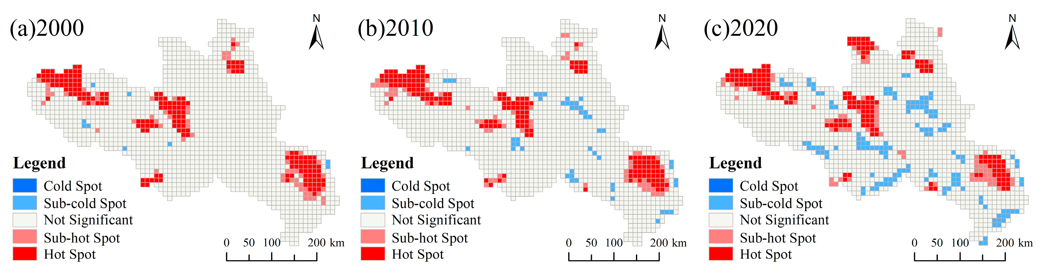
3.3. Local Spatial Auto-Correlation Analysis

In the three periods of 2000, 2010, and 2020, the Moran’s I of ecological risk index is positive, and the Z and p values are significant in the confidence interval. From 2000 to 2020, the spatial correlation of ecological risk in the landscape of the Yellow River source area and the aggregation pattern are mainly of “high–high” type and “low–low” type (Figure 6), i.e., there is an aggregation relationship between high-risk areas and high-risk areas, and an aggregation relationship between low-risk areas and low-risk areas. Meanwhile, Moran’s I of ecological risk index showed a trend of first increasing and then decreasing as time goes on, reaching a maximum value of 0.720 in 2010 and a minimum value of 0.681 in 2020, indicating that the spatial aggregation of the ecological risk index in the source region of the Yellow River first increased and then decreased, and the local difference first decreased and then increased.
The local spatial autocorrelation LISA plot (Figure 7) shows that the overall spatial aggregation of ecological risk indices is mainly “high–high” and “low–low” aggregation (positive correlation pattern), which is also consistent with the Moran’s I scatter plot results of ecological risk indices in the Yellow River source area. The “high–high” aggregation type is mainly distributed in the west (near the water area), the center (near the unused land), and the east (near the wetland). The “low–low” aggregation type shows a fragmented distribution. Statistics show that the “high–high” aggregation area accounted for 12.58% of the total study area, and the “low–high” aggregation area accounted for 0.47% of the total study area. The “low–low” aggregation accounted for 13.06% of the total study area. In 2010, the “high–high” aggregation accounted for 12.52% of the total study area, and the “low–high” aggregation accounted for 0.47% of the total study area. The “low–high” aggregation accounted for 0.34% of the total study area, and the “low–low” aggregation accounted for 15.68% of the total study area in 2010. In 2020, the “high–high” aggregation area accounted for 13.32% of the total study area, the “high–low” aggregation area accounted for 0.13% of the total study area, and the “low–high” aggregation area accounted for 0.34% of the total study area. From 2000 to 2020, there were some spatial differences in the characteristics of the aggregation areas of various ecological risk indices. Among them, the area of “high–high” and “low–low” aggregation zones decreased by 3.16%. The area of “high–high” and “low–low” clusters changed significantly, increasing by 0.74% and 2.42%, respectively; the area of “high–low” clusters increased slightly by 0.13%.
Overall, the Yellow River source area from 2000 to 2020 is mainly dominated by hot spot areas, with increasing sub-cold spot areas and fewer cold spot and sub-hot spot areas (Figure 8). The area of hot spot areas accounted for 11.78%, 11.37%, and 11.44% of the study area in 2000, 2010, and 2020, while the area of sub-hot spot areas accounted for 4.17%, 4.51%, and 5.25% of the study area. The area of the cold spot area accounts for 0.61%, 3.23%, and 9.35% of the study area. In terms of spatial distribution, the land types in the hot spot area are mainly water, unused land, and wetland, showing a high value aggregation pattern of ecological risk index. The sub-cold spot area has gradually increased since 2010, and its main land types are grassland, showing a low value aggregation pattern of ecological risk index. The cold spots, sub-cold spots, sub-hot spots, and hot spots of ecological risk in different areas of the Yellow River source area in the three time periods are still in the process of continuous transformation. The hot spot areas in the west are in a stable state, the hot spot areas in the north increased significantly in 2020, and the hot spot areas in the east are shrinking. In 2020, compared with 2000, the proportion of hot spot and sub-hot spot areas to the area of the study area increased by 0.74%, the proportion of cold spot and sub-cold spot areas to the area of the study area increased by 8.75%, and the area of sub-cold spot areas increased significantly. The above indicates that the ecological risk cold spot and hot spot areas are still in an unstable fluctuating state, and further rational adjustment of land use types and structures by anthropogenic or natural means should achieve the security and stability of the regional landscape ecosystem.

4. Discussion

Located in the southwest of China, the Tibet Plateau is an important ecological barrier protection key area in China due to its functions of water containment, soil conservation, wind and sand control, carbon fixation, and biodiversity conservation [40,41,42]. The Yellow River source area (YRSA) is on the southeastern edge of the Tibet Plateau and is the origin of the Yellow River basin, which plays an irreplaceable role in terms of water sources and has a very fragile ecological environment. Land use change is the most direct manifestation pattern of the interaction between human activities and the natural environment. The land itself is a macroscopic representation of the surface landscape, and its compositional structure or pattern changes are highly correlated with the spatial and temporal distribution and dynamics of ecological risks in the landscape. Therefore, the landscape pattern-based evaluation method is free from the inherent paradigm of traditional ecosystem evaluation to a certain extent. The method evaluates Landscape Ecological Risk (LER) directly from the spatial pattern at the regional scale, and the risk receptor changes from a single element in the ecosystem to the ecosystem itself that makes up the heterogeneous landscape [4]. There is growing evidence that environmental change has a strong influence on ecosystem processes and services on the Tibetan Plateau [43,44,45,46]. Climate change and land use change contributed positively to water supply between 2000 and 2008, with a 61% increase in the contribution of land use to increased water supply [47]. Due to the combined action of global warming and human activities, natural phenomena and anthropogenic behaviors can be seen as the main factors that cause desertification in the YRSA, with the increase in construction land and farmland in the north leading to increased desertification [48]. The average pH and NPP values of soils in the YRSA from 2000 to 2021 were low and showed a decreasing trend, indicating that the area has a weak carbon fixation capacity, and it was not conducive to the growth of vegetation [49,50]. The land use types in the YRSA are mainly grassland, including alpine grassland, degraded meadow, alpine meadow, and swampy meadow, and the changes in spatial structure are random and structural [51,52]. The grassland is constantly shifting to other land use types, and its transferred area is increasing as time goes on (Figure 3). The study shows that the land use types change more drastically after 2010 than before 2010, and the increase in the area of farmland and construction land is particularly obvious, with an increase of 228.40 km2 and 1712.06 km2, respectively, in 2020 compared to 2000. The area of unused land has increased by 2930.27 km2 in 20 years, which is due to the degradation and desertification of grassland caused by rampant rodents. As the water source of the Yellow River Basin, the source area contains many lakes and marshes and nurtures a variety of typical alpine ecosystems. The wetlands are the most important ecosystems in the source area, and they have the most biodiversity with a strong water-conserving capacity. Studies have shown that the water area and wetlands in the YRSA over the past 20 years have steadily increased by 260.89 km2 and 1094.93 km2, respectively. This phenomenon has secured the water supply of the Yellow River basin. Woodland plays an important role in the stability of the regional ecosystem, and protecting woodland can effectively protect biodiversity and water-catching capacity. However, because the natural environment of the YRSA is not conducive to the growth of woodland [53], woodland has the least area in the YRSA, with only 272.91 km2 in 2020. Over the past 20 years, the area of woodland first decreased, but then increasing.
In the 1980s, the land use mechanism in western cities was rigid, and the reform process lagged behind. With no unified land use management policy system. During this period, urban buildings showed low density with a low plot ratio and low yield of land. The emergence of the phenomenon of “enclose land for gardening” and the disorderly expansion of urban space made a great impact on the landscape pattern. Due to lack of attention to ecosystems by urban managers, natural landscapes such as farmland and grasslands have been encroached upon and destroyed by artificial landscapes, urban landscapes are fragmented, and the quality of natural ecosystems is reduced [54]. The study shows that the overall ecological risk in the YRSA is gradually increasing. There are differences in the changes in ecological risk values between regions. The ecological risk level in the northern region continues to rise because of the more frequent human activities in this region and the most construction land. As time goes on, the low ecological risk zone in the central part of the YRSA gradually upgrades to a medium-low ecological risk zone. During the study period, the land use type in such areas changed from grassland to unused land due to the intertwined effects of hydraulic and wind erosion in the YRSA, which led to the degradation and desertification of grassland. This phenomenon further exacerbates the rodent problem by destroying the living conditions of the rodents’ natural enemies. The decrease in the eastern high-risk area is due to the increase in wetlands, while the increase in the medium-high-risk area is due to the increase in farmland. Human activities and land use intensity in the YRSA are key factors contributing to the increase in ecological risk [55]. Figure 5 shows that ecological risk and land use intensity are positively correlated in areas where the area of construction land and farmland have increased significantly. Another way to state this is by saying that the ecological risk to the region increases significantly as the intensity of land use increases. The ecological risks in the YRSA show a clear spatial correlation; the main aggregation patterns are seen as “low–low” and “high–high”. The overall characteristic is high-risk and high-value. The “low–low” pattern has a fragmented distribution, where the landscape type is mainly grassland, far from construction sites and roads and other landscape stressors with low landscape separation and fragmentation, and a low intensity of anthropogenic disturbance. This pattern shows a low-risk value agglomeration and a relatively intact habitat. However, these areas have a low value of ecosystem services [56]. “The ‘high–high’ type has a concentrated distribution, where the landscape type is mainly water area, wetlands, and farmland with a high intensity of human and biological activities, and shows a high-risk agglomeration pattern. However, these areas have a high value of ecosystem services. After 20 years of change, from the view of the aggregation degree of cold and hot spots of ERI in the YRSA, the spatial distribution of high-value aggregation areas is stable with a small increase in the north, while there is a small decreasing trend in areas of high ERI in the east and west. The area of low-value aggregation areas increased by 8.75% in 2020 compared with 2000, showing a trend of year-on-year increase. In general, the spatial aggregation of the ERI in the YRSA gradually increased in terms of time scale, and the local variability gradually decreased. The risks of cold and hot spot areas are constantly changing, and the LER is still in an unstable fluctuation state. It is necessary to further adjust land use types and structures to enhance the stability of the regional landscape ecosystem.

5. Conclusions

In the last two decades, the ecological risk zones in the YRSA have been mainly low-risk, with a wide range of distribution and grassland being the main land use type. The high-risk areas are mainly water areas, unused land, and wetlands. In 2020, there were significant fluctuations in the size of the different levels of ecological risk zones, with a significant increase in the size of areas changing from low-risk to low-medium-risk and an increasing trend in LER. It is worth noting that ecological risk increases (Figure 5c) in areas where land use intensity increases (Figure 5a). The ERI cold spot areas show a significant increase in 2020 and are scattered, which was mainly due to the high altitude of the area, the predominantly grassland land, the low separation and fragmentation of the landscape, and the low intensity of human disturbance. In contrast, the ERI hot spots are concentrated, and their spatial distribution remains fixed. The land use types in the hot spot areas are mainly construction land, farmland, wetland, and water areas; the intensity of human activities is high, and the disturbance is strong. Therefore, it showed a concentration of high ecological risk values. In general, the ERI of the YRSA is increasing in the cold spot areas, while the hot spot areas are on a stable trend. However, the ecosystem landscape pattern in the study area is still unstable, and it is necessary to strengthen the control of the expansion of unused land and the intensity of human activities. This is to firmly implement ecological restoration policies such as afforestation and reforestation for stable ecosystem functions.
This paper intended to establish the link between changes in land use and landscape pattern and regional ecological risk by building up an evaluation index of landscape ecological risk and transforming landscape spatial structures into ecological risk variables through the spatial grid sampling method. This paper measured the degree of ecological risk in the Yellow River source area only from the perspective of landscape spatial structure without involving other natural or socio-economic factors. Therefore, there is no absoluteness regarding the calculated ecological risk values. However, the method of constructing an ecological risk index based on landscape pattern is feasible and effective to study the spatial pattern and dynamic changes of ecological risk in the watershed.

Author Contributions

Z.L. contributed to all aspects of this work. Q.S. contributed to the preparation of the framework and first draft of the study and supervision. J.Z. contributed to resource acquisition. All authors have read and agreed to the published version of the manuscript.

Funding

This research was funded by the Qinghai Province Basic Research Program Project, grant number 2021-ZJ-743.

Institutional Review Board Statement

Not applicable.

Informed Consent Statement

Not applicable.

Data Availability Statement

Not applicable.

Acknowledgments

Acknowledgement of funding from the Geological Resources and Geological Engineering discipline building project.

Conflicts of Interest

The authors declare no conflict of interest.

References

  1. He, G.; Ruan, J. Study on ecological security evaluation of Anhui Province based on normal cloud model. Environ. Sci. Pollut. Res. 2022, 29, 16549–16562. [Google Scholar] [CrossRef] [PubMed]
  2. Calow, P. Ecological risk assessment: Risk for what? How do we decide? Ecotoxicol. Environ. Saf. 1998, 40, 15–18. [Google Scholar] [CrossRef]
  3. van Loon-Steensma, J.M.; Goldsworthy, C. The application of an environmental performance framework for climate adaptation innovations on two nature-based adaptations. Ambio 2022, 51, 569–585. [Google Scholar] [CrossRef]
  4. Peng, J.; Dang, W.; Liu, Y.; Zong, M.; Hu, X. Review on landscape ecological risk assessment. Acta Geogr. Sin. 2015, 70, 664–677. [Google Scholar]
  5. Wu, L.Y. The Study of Regional Landscape Ecological Risk Assessment and the Environmental Risk Management Countermeasure: Take Dongshan Island for Example; Fujian Normal University: Fuzhou, China, 2004. [Google Scholar]
  6. Lawrence, A.K. Using landscape ecology to focus ecological risk assessment and guide risk management decision-making. Toxicol. Ind. Health 2001, 17, 236–246. [Google Scholar]
  7. Wang, G.; Cheng, G.; Qian, J. Several problems in ecological security assessment research. J. Appl. Ecol. 2003, 14, 1551–1556. [Google Scholar]
  8. Suter, G.W., II. Ecological Risk Assessment; CRC Press: Boca Raton, FL, USA, 2016. [Google Scholar]
  9. Li, L.; Fassnacht, F.E.; Bürgi, M. Using a landscape ecological perspective to analyze regime shifts in social–ecological systems: A case study on grassland degradation of the Tibetan Plateau. Landsc. Ecol. 2021, 36, 2277–2293. [Google Scholar] [CrossRef]
  10. Sahraoui, Y.; Leski, C.D.G.; Benot, M.-L.; Revers, F.; Salles, D.; van Halder, I.; Barneix, M.; Carassou, L. Integrating ecological networks modelling in a participatory approach for assessing impacts of planning scenarios on landscape connectivity. Landsc. Urban Plan. 2021, 209, 104039. [Google Scholar] [CrossRef]
  11. Zhang, F.; Yushanjiang, A.; Wang, D. Ecological risk assessment due to land use/cover changes (LUCC) in Jinghe County, Xinjiang, China from 1990 to 2014 based on landscape patterns and spatial statistics. Environ. Earth Sci. 2018, 77, 491. [Google Scholar] [CrossRef]
  12. De Montis, A.; Caschili, S.; Mulas, M.; Modica, G.; Ganciu, A.; Bardi, A.; Ledda, A.; Dessena, L.; Laudari, L.; Fichera, C.R. Urban–rural ecological networks for landscape planning. Land Use Policy 2016, 50, 312–327. [Google Scholar] [CrossRef]
  13. Zhang, W.; Chang, W.J.; Zhu, Z.C.; Hui, Z. Landscape ecological risk assessment of Chinese coastal cities based on land use change. Appl. Geogr. 2020, 117, 102174. [Google Scholar] [CrossRef]
  14. Xie, H.; Wen, J.; Chen, Q.; Wu, Q. Evaluating the landscape ecological risk based on GIS: A case-study in the poyang lake region of China. Land Degrad. Dev. 2021, 32, 2762–2774. [Google Scholar] [CrossRef]
  15. Liu, Y.; Liu, Y.; Li, J.; Lu, W.; Wei, X.; Sun, C. Evolution of landscape ecological risk at the optimal scale: A case study of the open coastal wetlands in Jiangsu, China. Int. J. Environ. Res. Public Health 2018, 15, 1691. [Google Scholar] [CrossRef] [Green Version]
  16. Ji, Y.; Bai, Z.; Hui, J. Landscape ecological risk assessment based on LUCC—A case study of Chaoyang county, China. Forests 2021, 12, 1157. [Google Scholar] [CrossRef]
  17. Wang, H.; Liu, X.; Zhao, C.; Chang, Y.; Liu, Y.; Zang, F. Spatial-temporal pattern analysis of landscape ecological risk assessment based on land use/land cover change in Baishuijiang National nature reserve in Gansu Province, China. Ecol. Indic. 2021, 124, 107454. [Google Scholar] [CrossRef]
  18. Ai, J.; Yu, K.; Zeng, Z.; Yang, L.; Liu, Y.; Liu, J. Assessing the dynamic landscape ecological risk and its driving forces in an island city based on optimal spatial scales: Haitan Island, China. Ecol. Indic. 2022, 137, 108771. [Google Scholar] [CrossRef]
  19. Li, C.; Zhang, J.; Philbin, S.P.; Yang, X.; Dong, Z.; Hong, J.; Ballesteros-Pérez, P. Evaluating the impact of highway construction projects on landscape ecological risks in high altitude plateaus. Sci. Rep. 2022, 12, 5170. [Google Scholar] [CrossRef] [PubMed]
  20. Yu, T.; Bao, A.; Xu, W.; Guo, H.; Jiang, L.; Zheng, G.; Yuan, Y.; Nzabarinda, V. Exploring variability in landscape ecological risk and quantifying its driving factors in the Amu Darya Delta. Int. J. Environ. Res. Public Health 2020, 17, 79. [Google Scholar] [CrossRef] [PubMed] [Green Version]
  21. Wu, L.; Liu, X.; Yang, Z.; Chen, J.; Ma, X. Landscape scaling of different land-use types, geomorphological styles, vegetation regionalizations, and geographical zonings differs spatial erosion patterns in a large-scale ecological restoration watershed. Environ. Sci. Pollut. Res. 2021, 28, 38374–38392. [Google Scholar] [CrossRef]
  22. Xia, M.; Jia, K.; Zhao, W.; Liu, S.; Wei, X.; Wang, B. Spatio-temporal changes of ecological vulnerability across the Qinghai-Tibetan Plateau. Ecol. Indic. 2021, 123, 107274. [Google Scholar] [CrossRef]
  23. Zhang, S.; Zhao, K.; Ji, S.; Guo, Y.; Wu, F.; Liu, J.; Xie, F. Evolution characteristics, eco-environmental response and influencing factors of production-living-ecological space in the Qinghai–Tibet Plateau. Land 2022, 11, 1020. [Google Scholar] [CrossRef]
  24. Wang, S.; Wei, Y. Qinghai-tibetan plateau greening and human well-being improving: The role of ecological policies. Sustainability 2022, 14, 1652. [Google Scholar] [CrossRef]
  25. Cai, H.; Yang, X.; Xu, X. Human-induced grassland degradation/restoration in the central Tibetan Plateau: The effects of ecological protection and restoration projects. Ecol. Eng. 2015, 83, 112–119. [Google Scholar] [CrossRef]
  26. Jun, C.; Ban, Y.; Li, S. Open access to Earth land-cover map. Nature 2014, 514, 434. [Google Scholar] [CrossRef] [Green Version]
  27. GB/T 21010-2017; Current Land Use Classification. General Administration of Quality Supervision, Inspection and Quarantine of the People’s Republic of China. China National Standardization Administration: Beijing, China, 2017.
  28. Zhang, H.; Wang, Z.; Chai, J. Land use\cover change and influencing factors inside the urban development boundary of different level cities: A case study in Hubei Province, China. Heliyon 2022, 8, e10408. [Google Scholar] [CrossRef]
  29. Hu, Y.; Zhen, L.; Zhuang, D. Assessment of land-use and land-cover change in Guangxi, China. Sci. Rep. 2019, 9, 2189. [Google Scholar] [CrossRef] [PubMed] [Green Version]
  30. GB/T 12409-2009; Geographic Grid. General Administration of Quality Supervision, Inspection and Quarantine of the People’s Republic of China. China National Standardization Administration: Beijing, China, 2009.
  31. Chen, X.; Xie, G.; Zhang, J. Landscape ecological risk assessment of land use changes in the coastal area of Haikou City in the past 30 years. Acta Ecol. Sin. 2021, 41, 975–986. [Google Scholar]
  32. Du, J.; Zhao, S.; Qiu, S.; Guo, L. Land Use Change and Landscape Ecological Risk Assessment in Loess Hilly Region of Western Henan Province from 2000 to 2015. Res. Soil Water Conserv. 2021, 28, 279–284+291. [Google Scholar]
  33. Jin, X.; Jin, Y.; Mao, X. Ecological risk assessment of cities on the Tibetan Plateau based on land use/land cover changes–Case study of Delingha City. Ecol. Indic. 2019, 101, 185–191. [Google Scholar] [CrossRef]
  34. Kang, Z.; Zhang, Z.; Wei, H.; Liu, L.; Ning, S.; Zhao, G.; Wang, T.; Tian, H. Landscape ecological risk assessment in Manas River Basin based on land use change. Acta Ecol. Sin. 2020, 40, 6472–6485. [Google Scholar]
  35. Yang, L.; Deng, M.; Wang, J.; Jue, H. Spatial-temporal evolution of land use and ecological risk in Dongting Lake Basin during 1980–2018. Acta Ecol. Sin. 2021, 41, 3929. [Google Scholar]
  36. Shen, Z.; Zeng, J. Spatial relationship of urban development to land surface temperature in three cities of southern Fujian. Acta Geogr. Sin. 2021, 76, 566–583. [Google Scholar]
  37. Qiu, B.; Wang, Q.; Chen, C.; Chi, T. Spatial Autocorr elation Analysis of Multi-scale Land Use in Fujian Province. J. Nat. Resour. 2007, 22, 311–321. [Google Scholar]
  38. Cohen, I.; Huang, Y.; Chen, J.; Benesty, J.; Benesty, J.; Chen, J.; Huang, Y.; Cohen, I. Pearson correlation coefficient. In Noise Reduction in Speech Processing; Springer: Berlin/Heidelberg, Germany, 2009; pp. 1–4. [Google Scholar]
  39. Hoque, M.Z.; Islam, I.; Ahmed, M.; Hasan, S.S.; Prodhan, F.A. Spatio-temporal changes of land use land cover and ecosystem service values in coastal Bangladesh. Egypt. J. Remote Sens. Space Sci. 2022, 25, 173–180. [Google Scholar]
  40. Fu, B.; Ouyang, Z.; Shi, P.; Fan, J.; Wang, X.; Zheng, H.; Zhao, W.; Wu, F. Current Condition and Protection Strategies of Qinghai-Tibet Plateau Ecological Security Barrier. China Acad. J. Electron. Publ. House 2021, 36, 1298–1306. [Google Scholar]
  41. Xue, J.; Li, Z.; Feng, Q.; Gui, J.; Zhang, B. Spatiotemporal variations of water conservation and its influencing factors in ecological barrier region, Qinghai-Tibet Plateau. J. Hydrol. Reg. Stud. 2022, 42, 101164. [Google Scholar] [CrossRef]
  42. Zhao, Y.; Chen, D.; Fan, J. Sustainable development problems and countermeasures: A case study of the Qinghai-Tibet Plateau. Geogr. Sustain. 2020, 1, 275–283. [Google Scholar] [CrossRef]
  43. Hu, Y.; Maskey, S.; Uhlenbrook, S. Trends in temperature and rainfall extremes in the Yellow River source region, China. Clim. Change 2012, 110, 403–429. [Google Scholar] [CrossRef] [Green Version]
  44. Ni, Y.; Lv, X.; Yu, Z.; Wang, J.; Ma, L.; Zhang, Q. Intra-annual variation in the attribution of runoff evolution in the Yellow River source area. Catena 2023, 225, 107032. [Google Scholar] [CrossRef]
  45. Qin, Y.; Yang, D.; Gao, B.; Wang, T.; Chen, J.; Chen, Y.; Wang, Y.; Zheng, G. Impacts of climate warming on the frozen ground and eco-hydrology in the Yellow River source region, China. Sci. Total Environ. 2017, 605, 830–841. [Google Scholar] [CrossRef] [Green Version]
  46. Tian, H.; Lan, Y.; Wen, J.; Jin, H.; Wang, C.; Wang, X.; Kang, Y. Evidence for a recent warming and wetting in the source area of the Yellow River (SAYR) and its hydrological impacts. J. Geogr. Sci. 2015, 25, 643–668. [Google Scholar] [CrossRef]
  47. Pan, T.; Wu, S.; Liu, Y. Relative contributions of land use and climate change to water supply variations over yellow river source area in Tibetan plateau during the past three decades. PLoS ONE 2015, 10, e0123793. [Google Scholar] [CrossRef]
  48. Guo, B.; Wei, C.; Yu, Y.; Liu, Y.; Li, J.; Meng, C.; Cai, Y. The dominant influencing factors of desertification changes in the source region of Yellow River: Climate change or human activity? Sci. Total Environ. 2022, 813, 152512. [Google Scholar] [CrossRef]
  49. Rong, T.; Long, L.H. Quantitative Assessment of NPP Changes in the Yellow River Source Area from 2001 to 2017. IOP Conf. Ser. Earth Environ. Sci. 2021, 687, 012002. [Google Scholar] [CrossRef]
  50. Zhang, X.; Nian, L.; Liu, X.; Li, X.; Adingo, S.; Liu, X.; Wang, Q.; Yang, Y.; Zhang, M.; Hui, C. Spatial–Temporal Correlations between Soil pH and NPP of Grassland Ecosystems in the Yellow River Source Area, China. Int. J. Environ. Res. Public Health 2022, 19, 8852. [Google Scholar] [CrossRef] [PubMed]
  51. Liu, J.; Chen, J.; Qin, Q.; You, H.; Han, X.; Zhou, G. Patch pattern and ecological risk assessment of alpine grassland in the source region of the Yellow River. Remote Sens. 2020, 12, 3460. [Google Scholar] [CrossRef]
  52. McDaniels, T.; Axelrod, L.J.; Slovic, P. Characterizing perception of ecological risk. Risk Anal. 1995, 15, 575–588. [Google Scholar] [CrossRef] [PubMed] [Green Version]
  53. Jin, H.; He, R.; Cheng, G.; Wu, Q.; Wang, S.; Lü, L.; Chang, X. Changes in frozen ground in the Source Area of the Yellow River on the Qinghai–Tibet Plateau, China, and their eco-environmental impacts. Environ. Res. Lett. 2009, 4, 045206. [Google Scholar] [CrossRef]
  54. Wu, T.; Hou, X.; Xu, X. Spatio-temporal characteristics of the mainland coastline utilization degree over the last 70 years in China. Ocean Coast. Manag. 2014, 98, 150–157. [Google Scholar] [CrossRef]
  55. Du, L.; Dong, C.; Kang, X.; Qian, X.; Gu, L. Spatiotemporal evolution of land cover changes and landscape ecological risk assessment in the Yellow River Basin, 2015–2020. J. Environ. Manag. 2023, 332, 117149. [Google Scholar] [CrossRef]
  56. Lu, Z.; Song, Q.; Zhao, J.; Wang, S. Prediction and Evaluation of Ecosystem Service Value Based on Land Use of the Yellow River Source Area. Sustainability 2022, 15, 687. [Google Scholar] [CrossRef]
Figure 1. Overview of the study area and delineation of risk neighborhood.
Sustainability 15 09749 g001
Figure 2. Spatial distribution of land use. (The solid line in the graph shows the trend of the different land use types 10 years apart and the dashed line shows the trend line of the different land use types over a period of 21 years.)
Sustainability 15 09749 g002
Figure 3. Land use transfer Sankey map.
Sustainability 15 09749 g003
Figure 4. Spatial distribution of ecological risk levels.
Sustainability 15 09749 g004
Figure 5. Correlation analysis of land use intensity and ERI change. ((a) is the change in land use intensity, (b) is the change in Ecological Risk Index, (c) is correlation co-efficient r value, (d) is the significance p value).
Sustainability 15 09749 g005
Figure 6. Moran’s I scatter diagram.
Sustainability 15 09749 g006
Figure 7. Aggregation and outlier analysis graphs. (“High–High Cluster” shows as high values around high values, “High–Low Outlier” shows as low values around high values, “Low–Low Cluster” shows as low values around low values, “Low–High Outlier” shows as high values around low values).
Sustainability 15 09749 g007
Figure 8. Hot spot analysis graph. (The confidence interval between cold spots and hot spots is more than 99%, while confidence interval between sub-hot and sub-cold spots is between 90% and 95%).
Sustainability 15 09749 g008
Table 1. Land use type classification and intensity.
Macro LULC ClassesMicro LULC Classes InformationLevel of Intensity
Construction landSurface formed by man-made construction activities, including various residential areas, industrial mines, and transportation facilities in towns.7
FarmlandLand used for growing crops, including paddy fields, dry land, vegetable fields, pastureland, orchards.6
WoodlandThe land is covered by trees with crown coverage over 30% and the land covered by shrubs with shrub coverage over 30% are forest, shrub land, open forest land, and immature forest land.5
GrasslandThe land covered by natural herbaceous vegetation with coverage higher than 10% includes grassland, meadow, savanna, and desert grassland.4
WetlandLand with shallow water or over-wet soil, including inland marshes, lake marshes, and shrub wetlands.3
WaterLiquid water covered areas and ice-covered areas, including rivers, lakes, glaciers, and beaches.2
Unused landNaturally covered land with less than 10% vegetation cover, including saline, sandy, bare rock, and bare tundra.1
Table 2. Calculation method of landscape pattern index.
IndexSymbolFormula
Landscape fragmentation F i F i = n i A i
In the formula, n i is the number of patches of landscape type i , A i is the area of landscape type i .
Landscape Separation S i S i = l i × A A i , l i = 1 2 n i A
In the formula, l i is the distance index of landscape type I , A is the total area of landscape type i
Landscape fractal dimension F D i F D i = 2 ln P i 4 ln A i
In the formula, P i is the perimeter of the landscape type i
Landscape disturbance degree D i D i = a F i + b S i + c F D i
In the formula, a, b, and c are the weights of the corresponding landscape indices, and a + b + c = 1
Landscape Vulnerability V i The vulnerability index of each landscape type itself after normalization after scoring by experts are farmland, 0.14, woodland, 0.07, grassland, 0.11, wetland, 0.18, water, 0.21, construction land, 0.04, and unused land, 0.25
Landscape loss degree R i R i = D i × V i
Disclaimer/Publisher’s Note: The statements, opinions and data contained in all publications are solely those of the individual author(s) and contributor(s) and not of MDPI and/or the editor(s). MDPI and/or the editor(s) disclaim responsibility for any injury to people or property resulting from any ideas, methods, instructions or products referred to in the content.

