


Towards Sustainable Safe Driving: A Multimodal Fusion Method for Risk Level Recognition in Distracted Driving Status


Abstract
1. Introduction
2. Materials and Methods
2.1. Data Collection
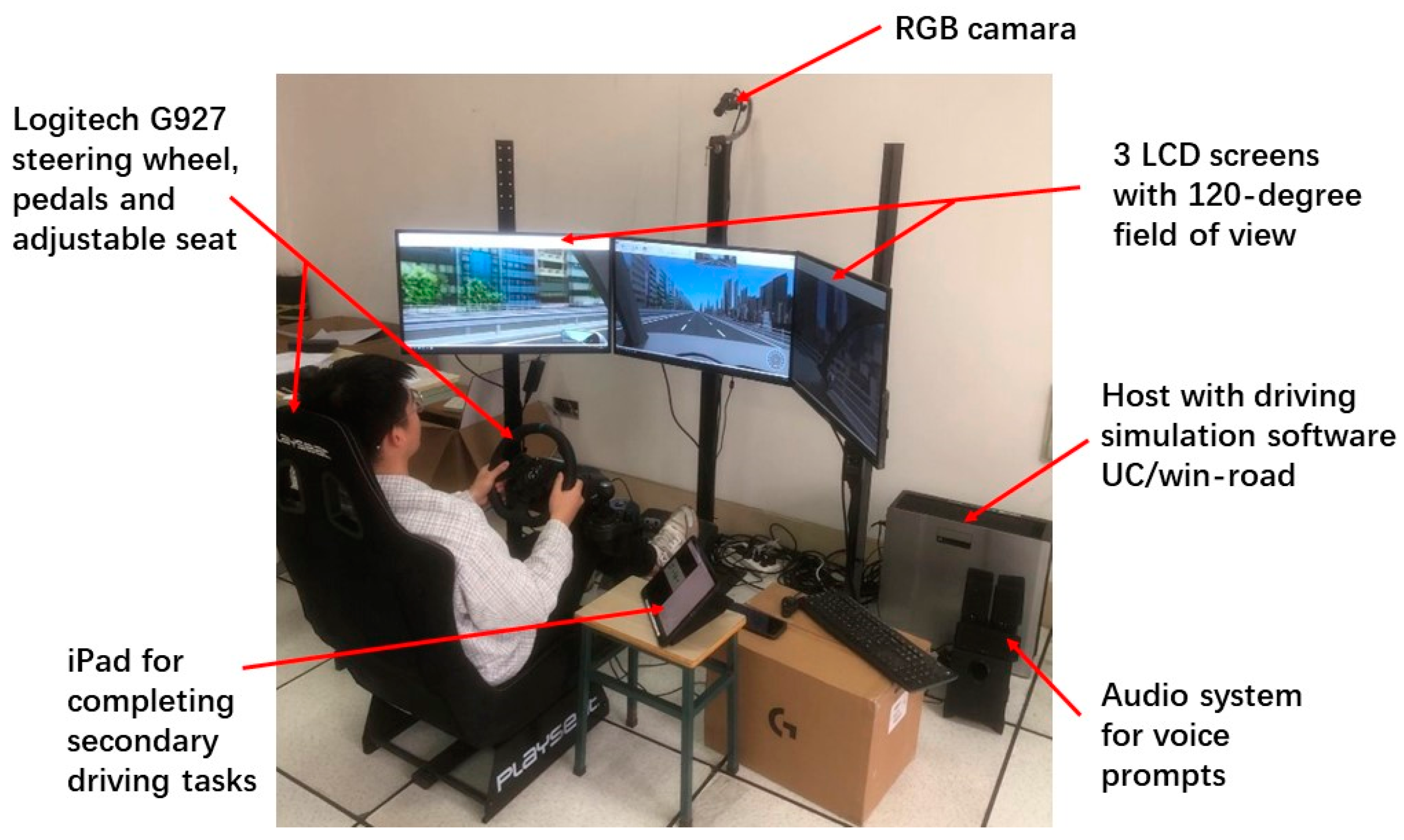
2.1.1. Driving Simulation Platform
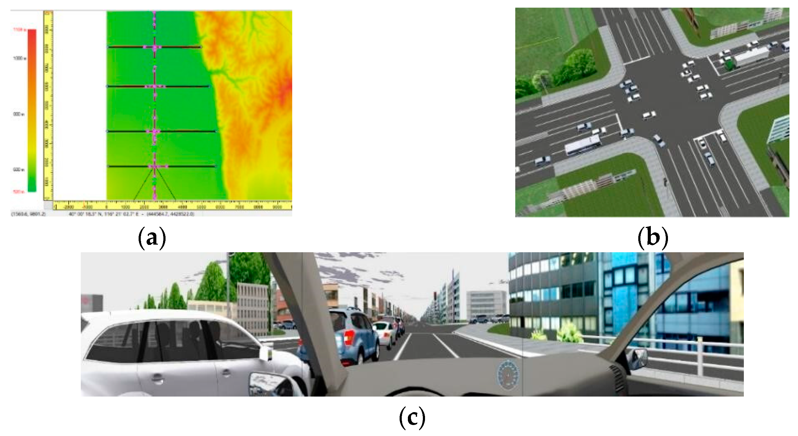
2.1.2. Participants and Driving Scenarios
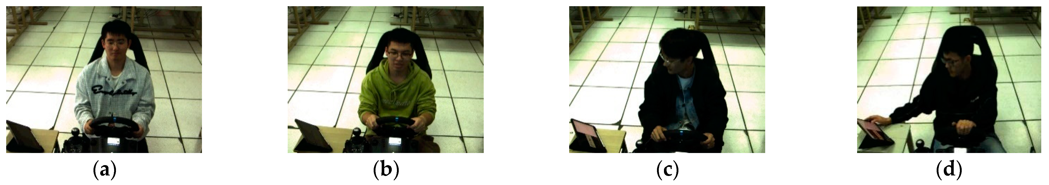
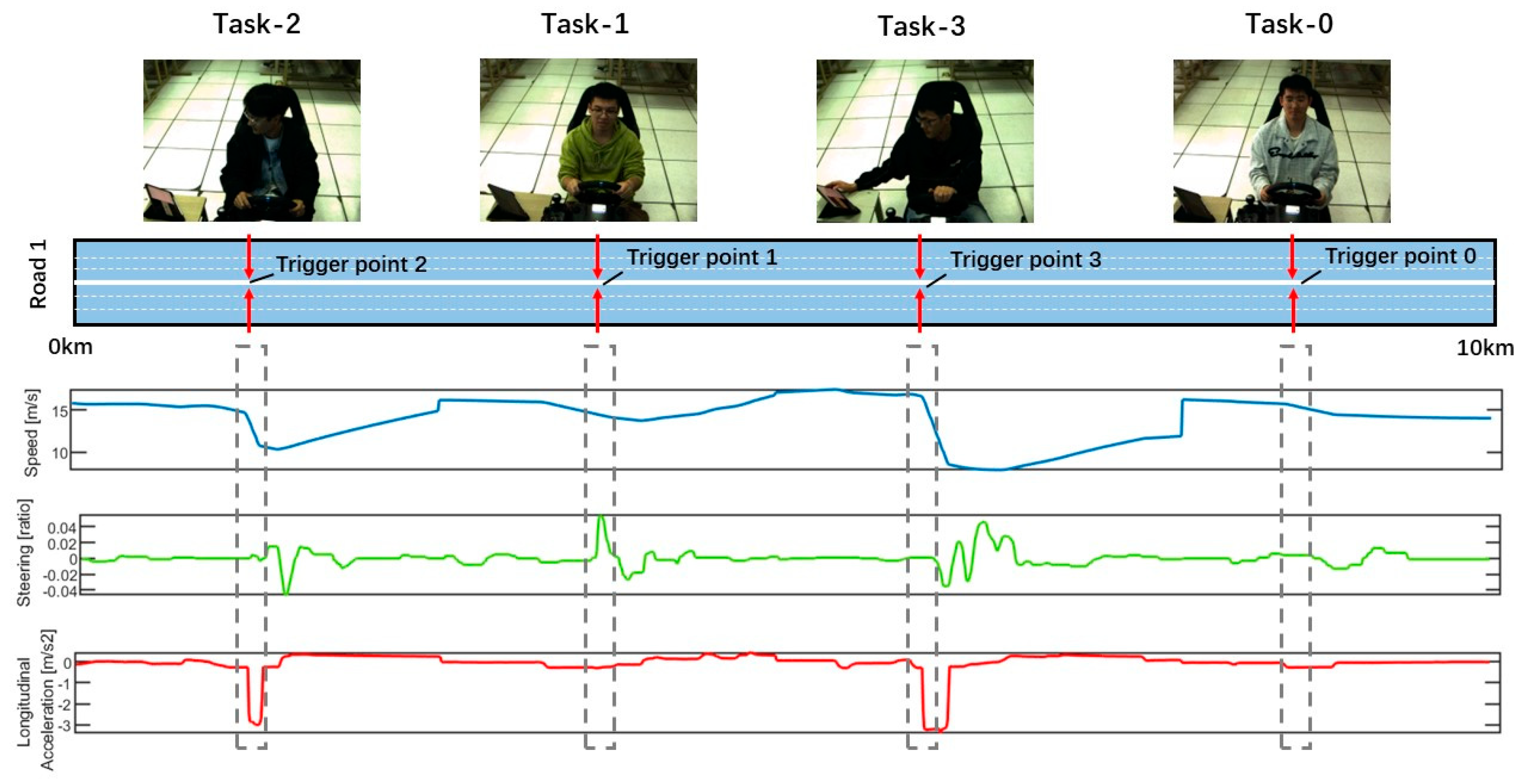
2.1.3. Secondary Task
2.1.4. Procedure
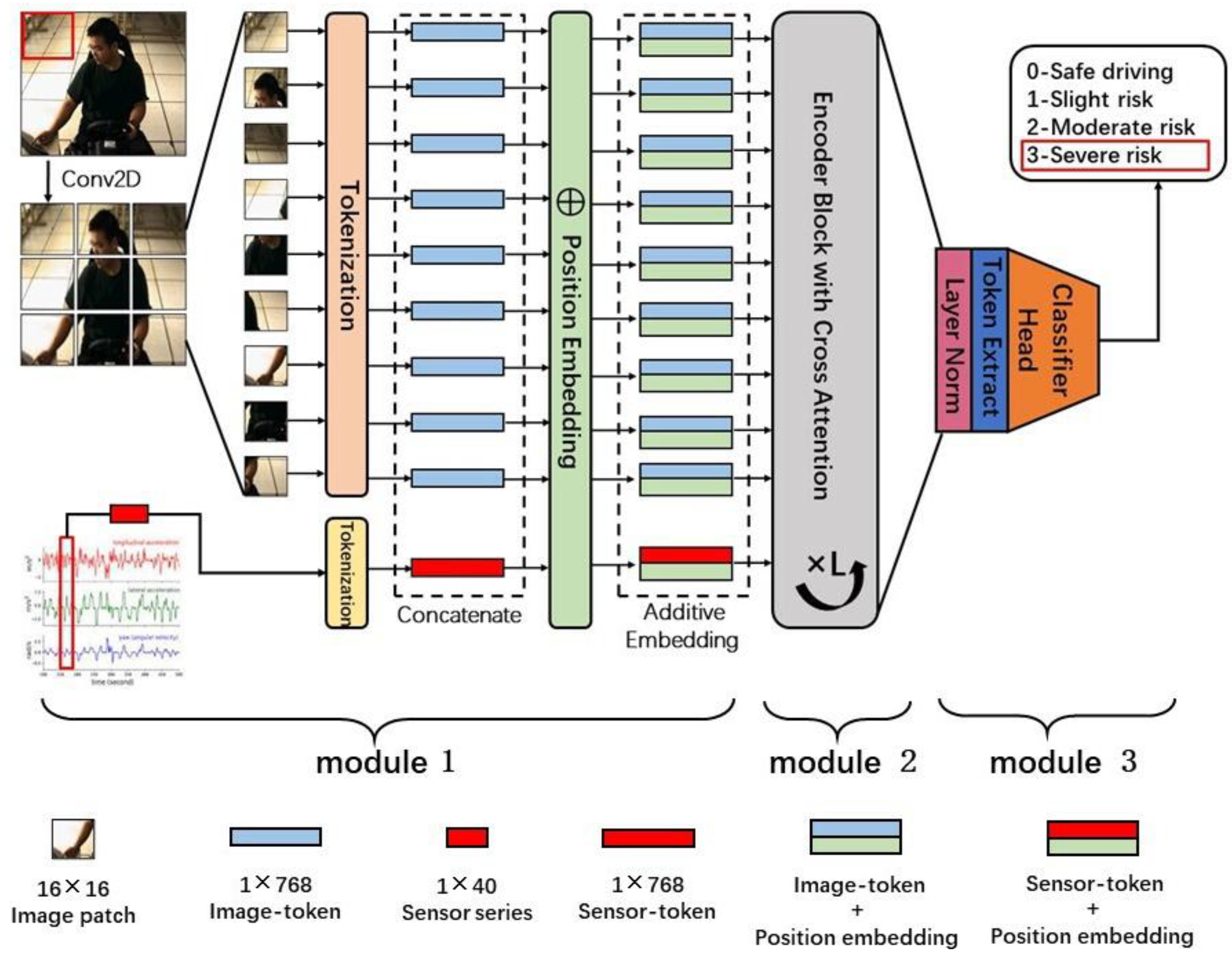
2.2. Methods
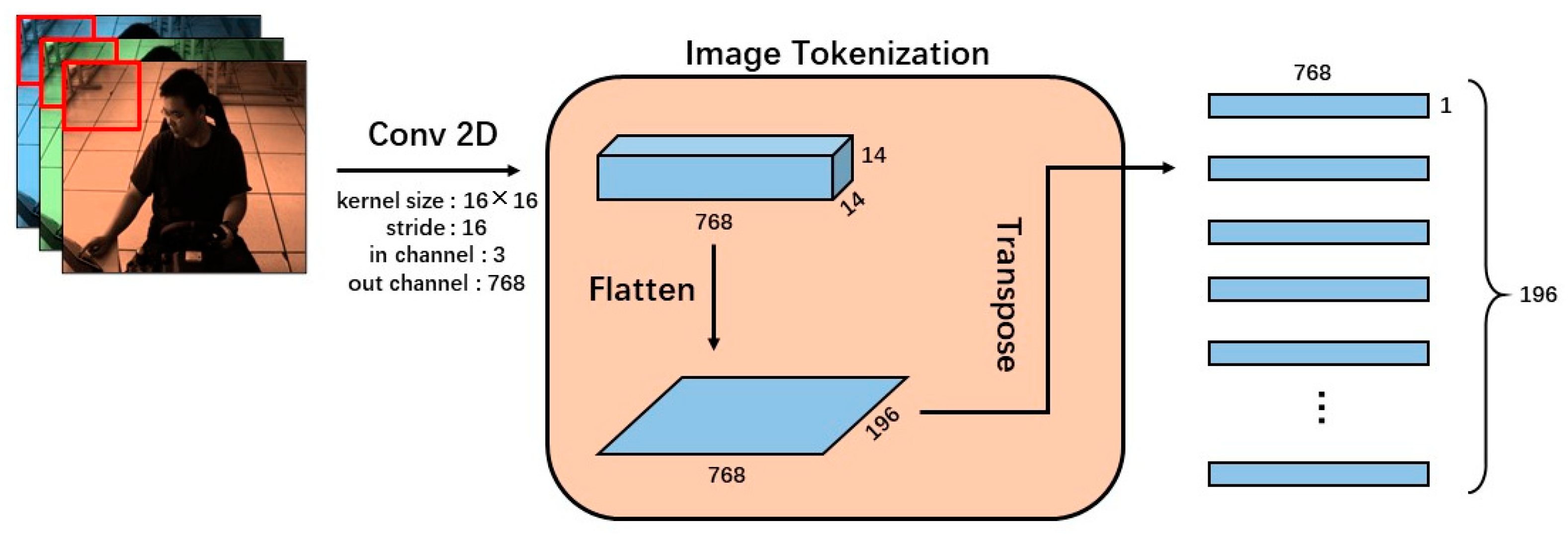
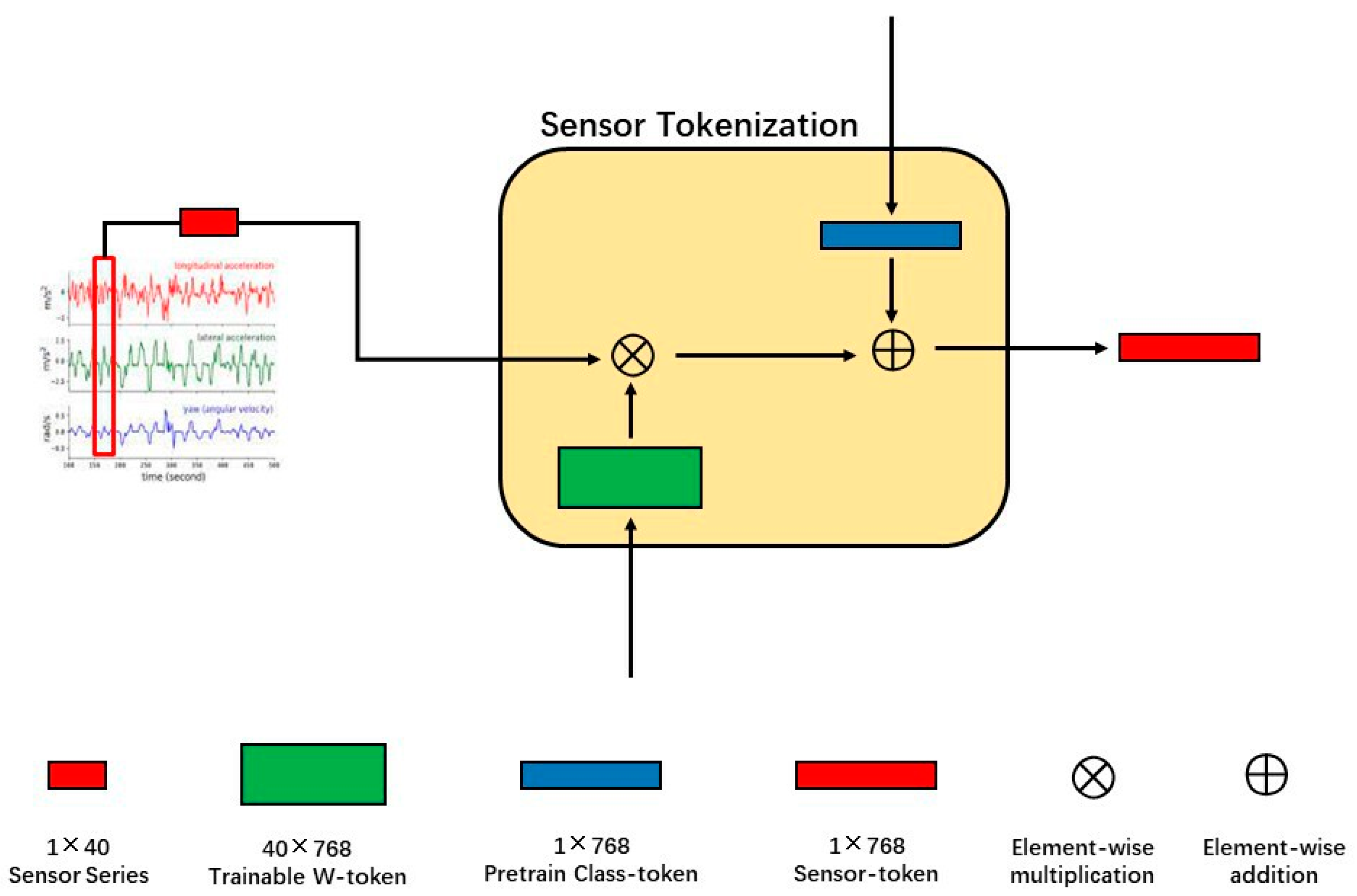
2.2.1. Module 1: Early Fusion of Vision-Modal Data and Sensor-Modal Data
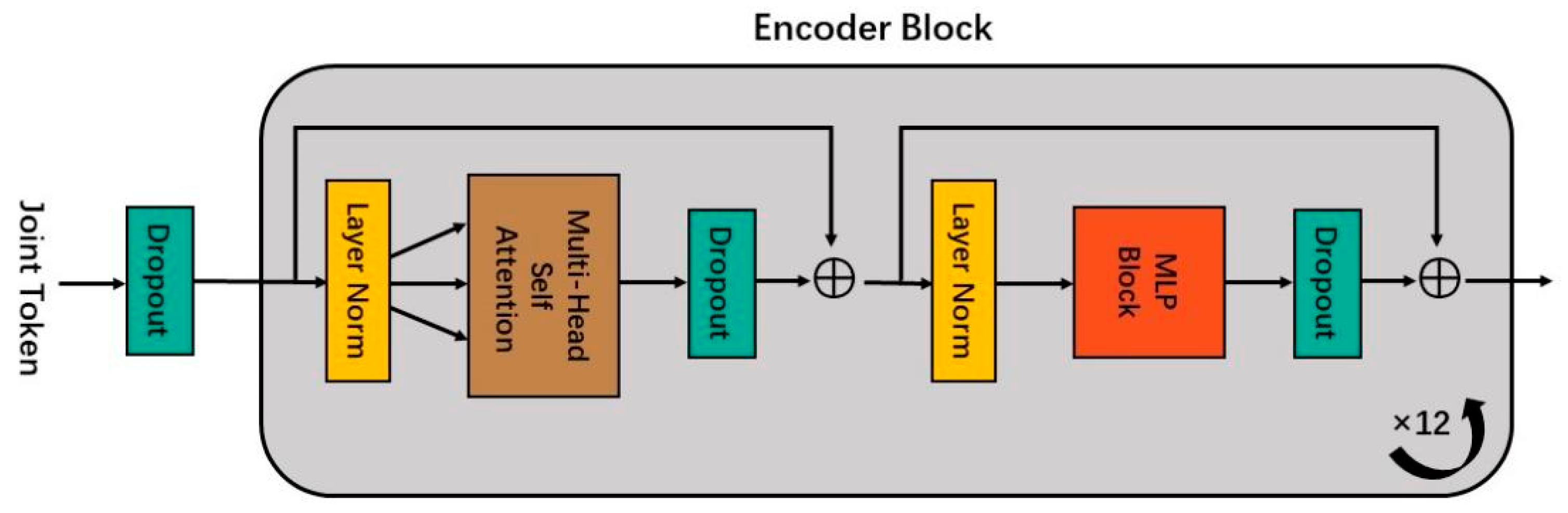
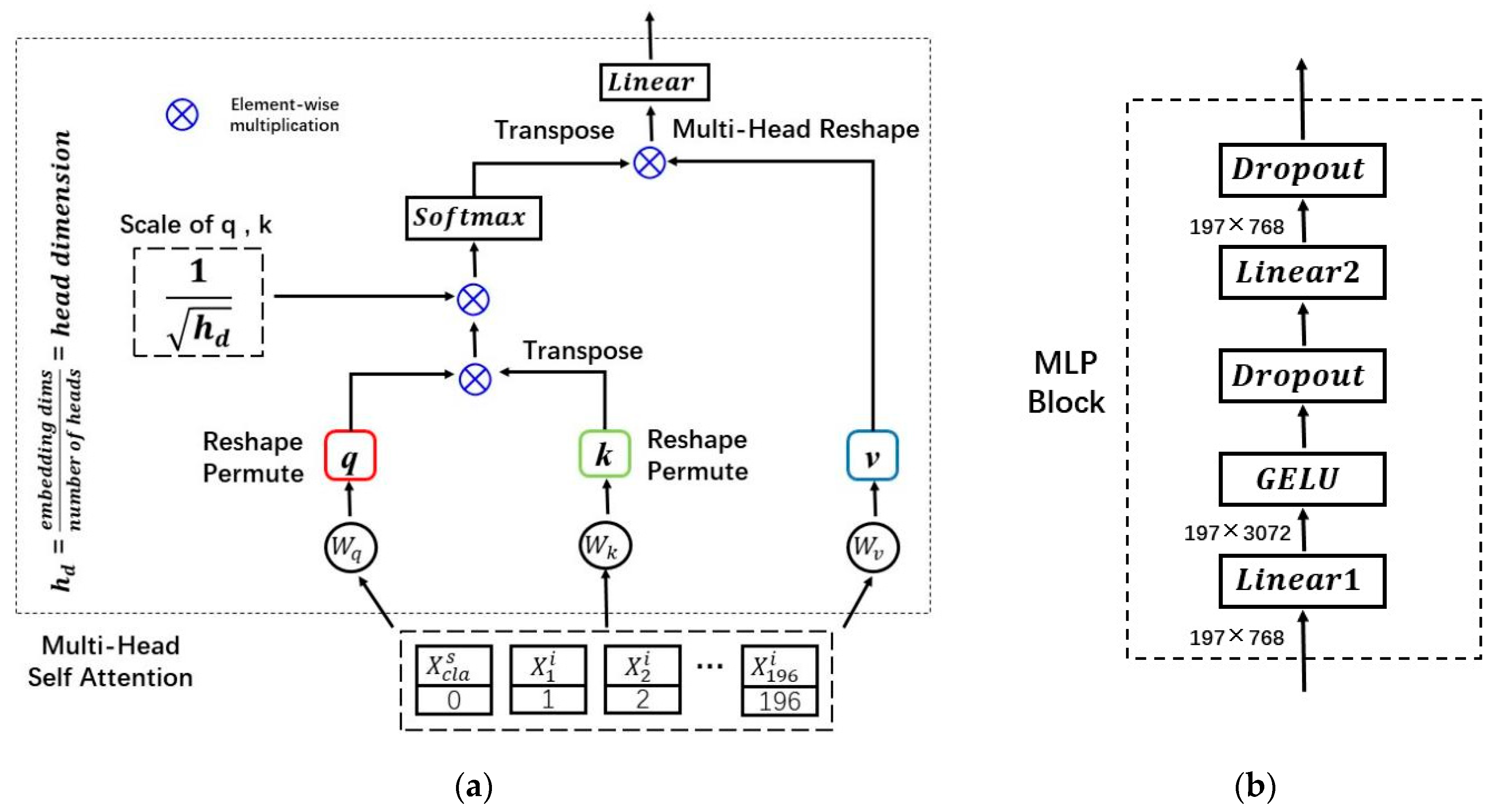
2.2.2. Module 2: Modality Information Interaction in the Encoder Block
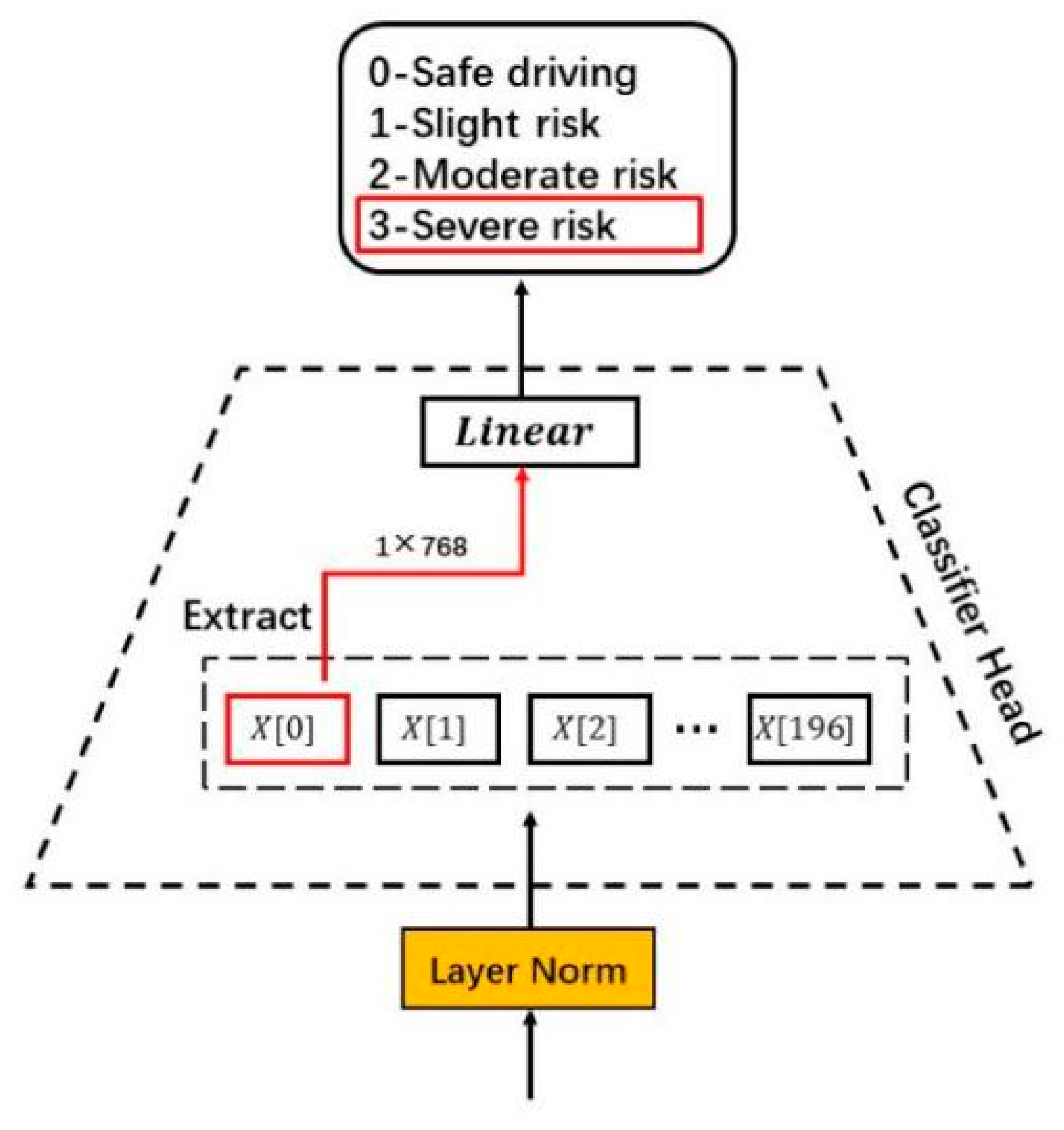
2.2.3. Module 3: Classifier Head for Risk Level Inference
2.3. Evaluation Metrics
3. Results
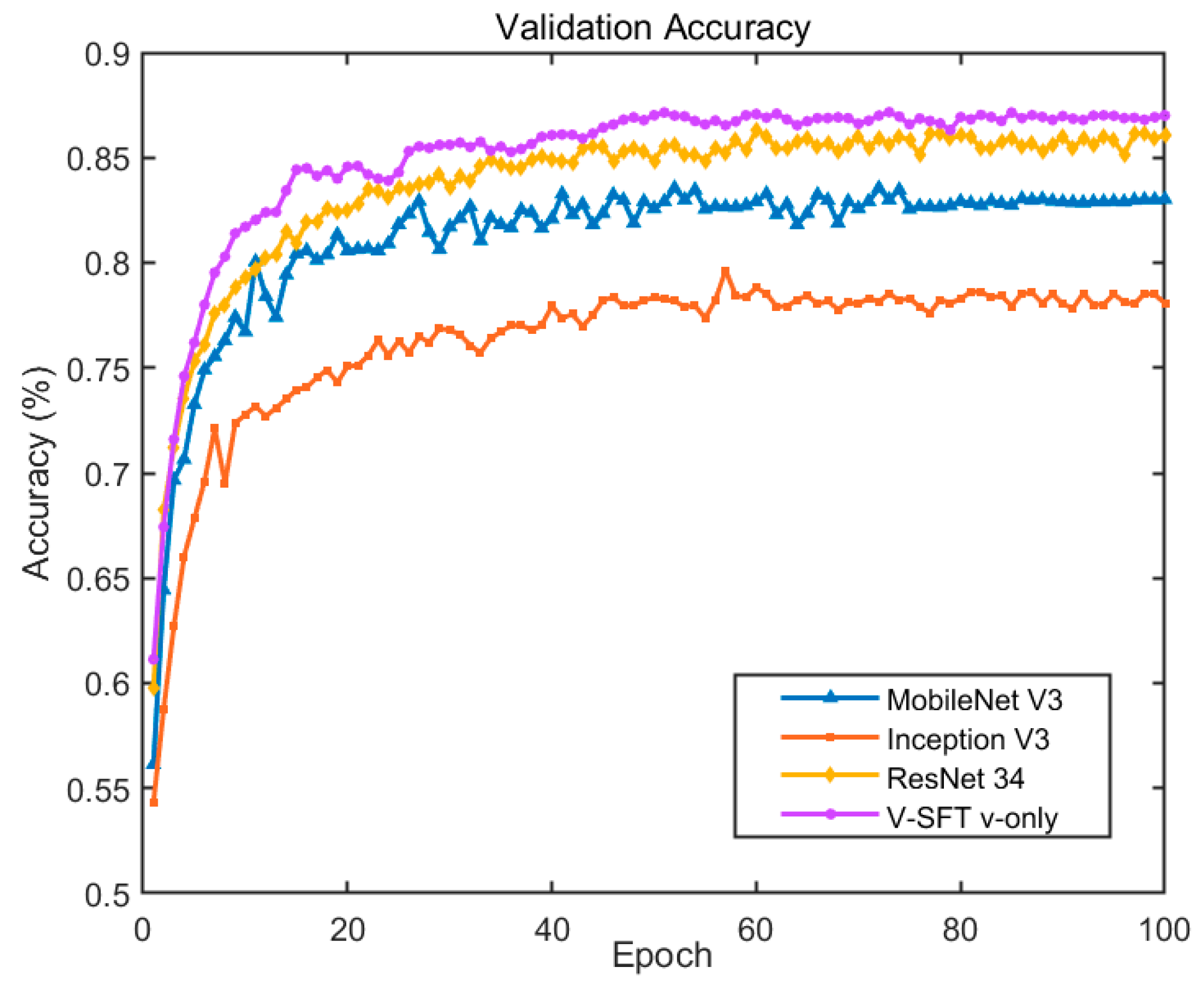
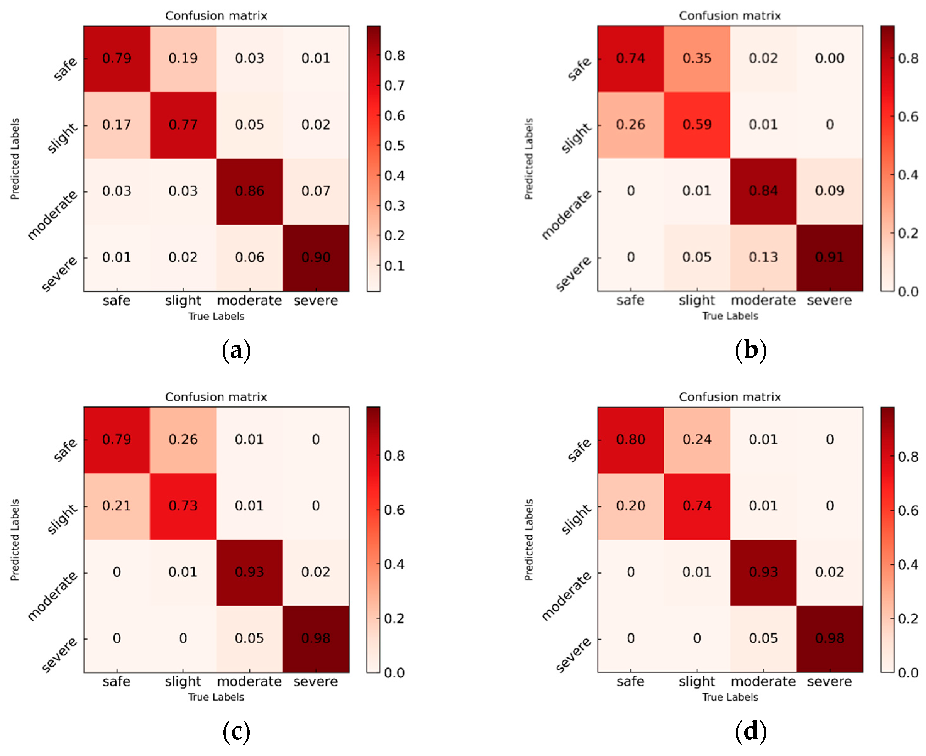
3.1. Experimental Evaluation of Vision-Only Modality Input
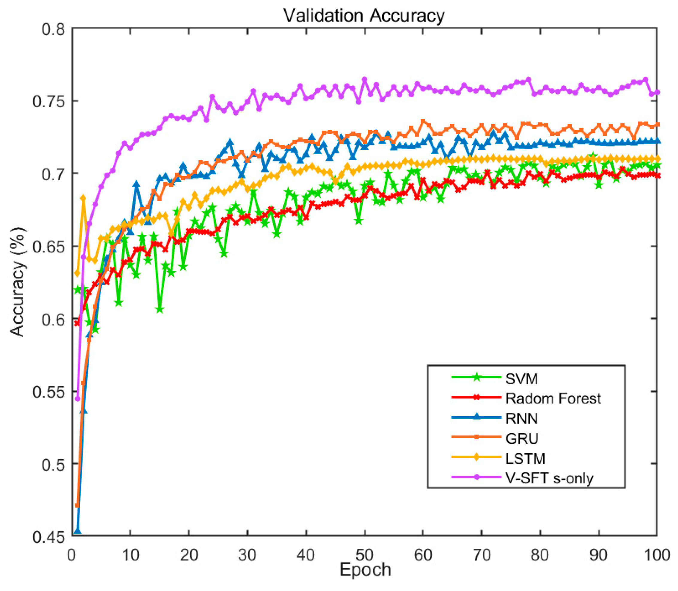
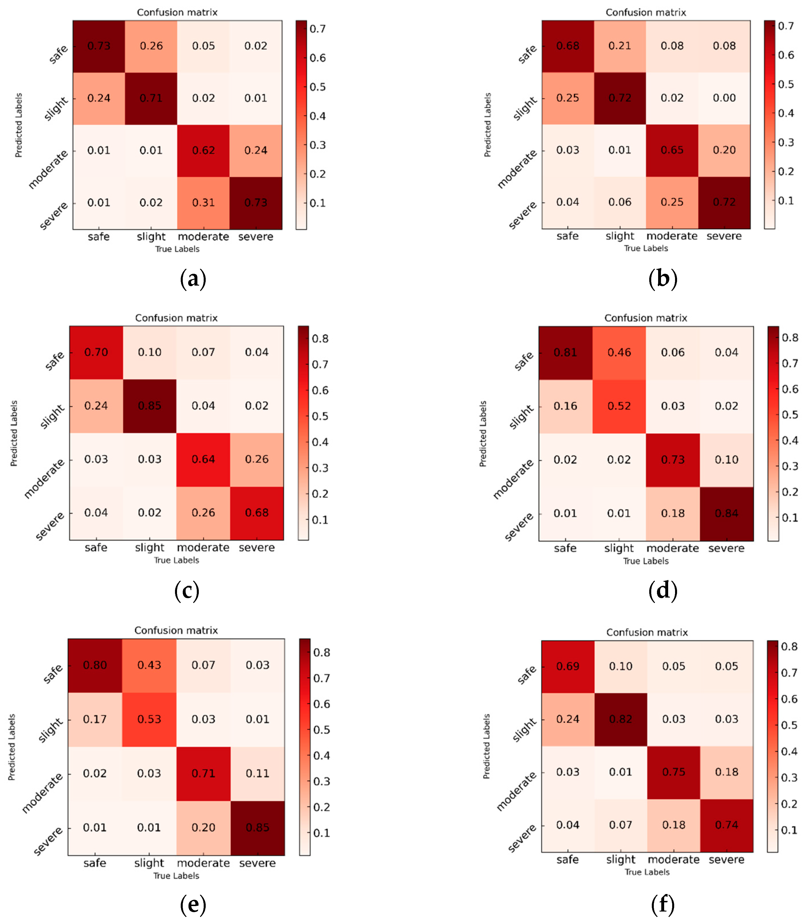
3.2. Experimental Evaluation of Sensor-Only Modality Input
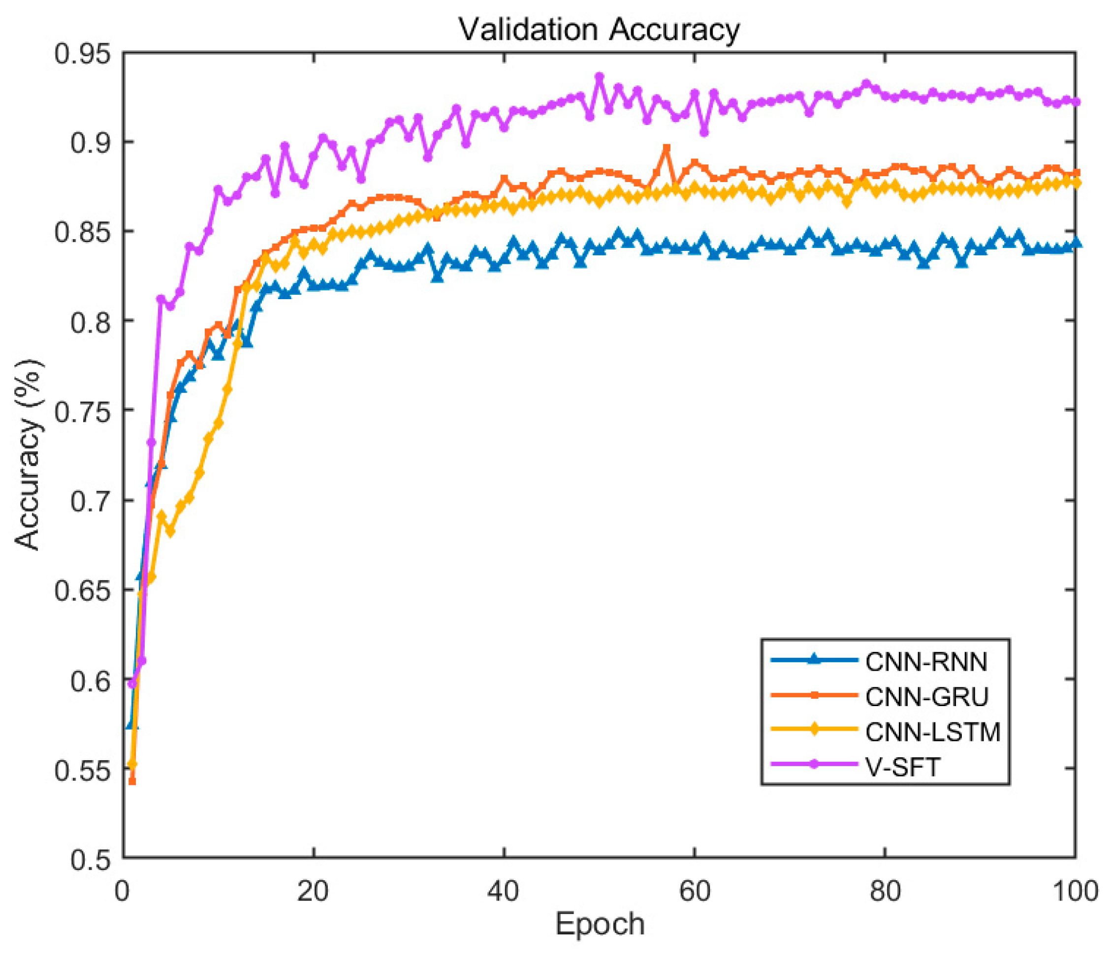
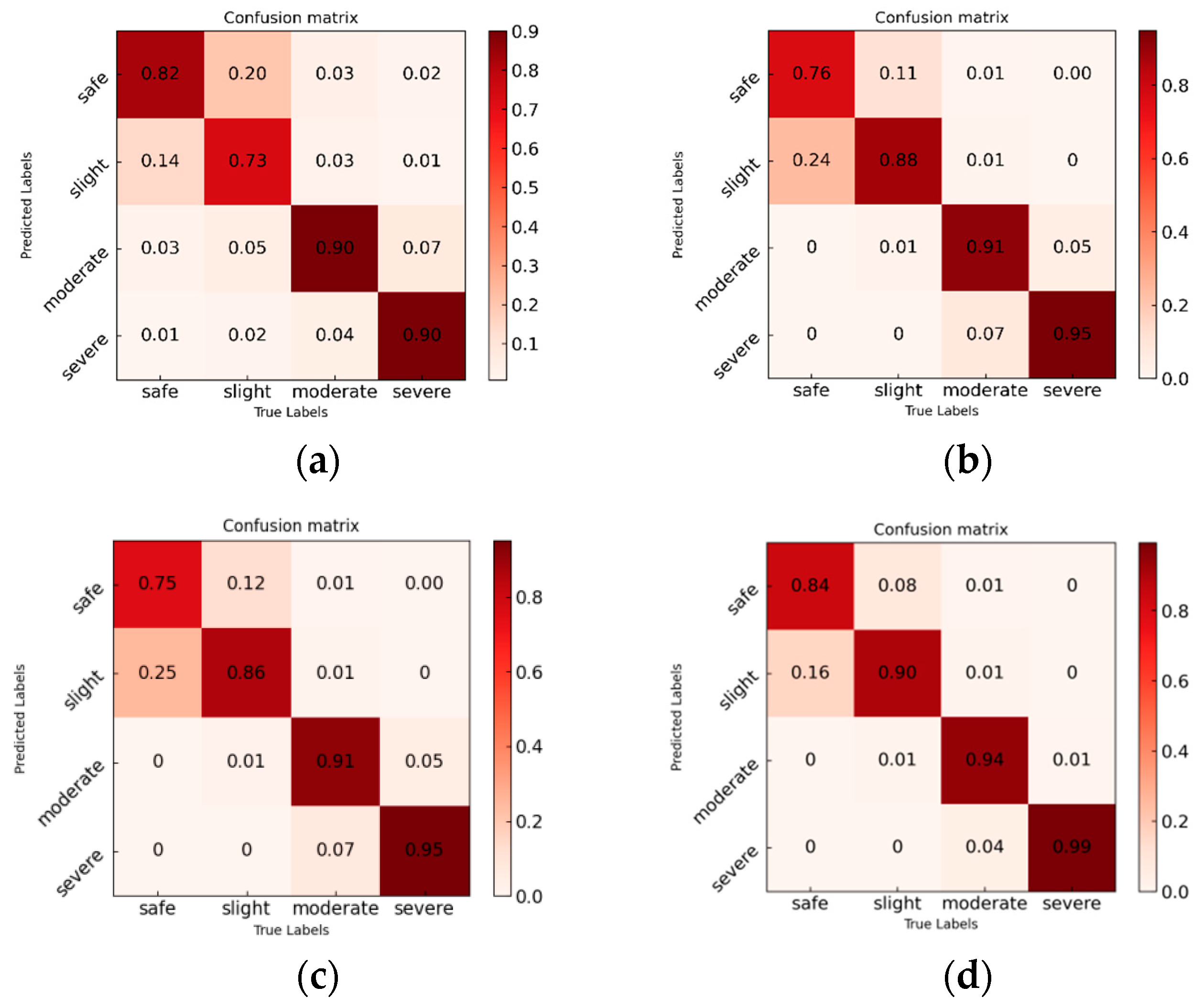
3.3. Experimental Evaluation for Vision-Sensor Multimodal Data Input
4. Discussion
5. Conclusions
Author Contributions
Funding
Institutional Review Board Statement
Informed Consent Statement
Data Availability Statement
Acknowledgments
Conflicts of Interest
References
- Hu, Y.; Qu, T.; Liu, J.; Shi, Z.Q.; Zhu, B.; Cao, D.P.; Chen, H. human-machine cooperative control of intelligent vehicle: Recent developments and future perspectives. Acta Autom. Sin. 2019, 45, 1261–1280. [Google Scholar]
- Xian, H.; Hou, Y.; Wang, Y.; Dong, S.; Kou, J.; Li, Z. Influence of Risky Driving Behavior and Road Section Type on Urban Expressway Driving Safety. Sustainability 2022, 15, 398. [Google Scholar] [CrossRef]
- Distracted Driving Statistics. 2022. Available online: https://www.bankrate.com/insurance/car/distracted-driving-statistics (accessed on 9 August 2022).
- Rahman, M.M.; Islam, M.K.; Al-Shayeb, A.; Arifuzzaman, M. Towards sustainable road safety in Saudi Arabia: Exploring traffic accident causes associated with driving behavior using a Bayesian belief network. Sustainability 2022, 14, 6315. [Google Scholar] [CrossRef]
- Sayed, I.; Abdelgawad, H.; Said, D. Studying driving behavior and risk perception: A road safety perspective in Egypt. J. Eng. Appl. Sci. 2022, 69, 22. [Google Scholar] [CrossRef]
- Suzuki, K.; Tang, K.; Alhajyaseen, W.; Suzuki, K.; Nakamura, H. An international comparative study on driving attitudes and behaviors based on questionnaire surveys. IATSS Res. 2022, 46, 26–35. [Google Scholar] [CrossRef]
- Wang, L.; Wang, Y.; Shi, L.; Xu, H. Analysis of risky driving behaviors among bus drivers in China: The role of enterprise management, external environment and attitudes towards traffic safety. Accid. Anal. Prev. 2022, 168, 106589. [Google Scholar] [CrossRef] [PubMed]
- Ge, H.M.; Zheng, M.Q.; Lv, N.C.; Lu, Y.; Sun, H. Review on driving distraction. J. Traffic Transp. Eng. 2021, 21, 38–55. [Google Scholar]
- Li, N.; Busso, C. Predicting perceived visual and cognitive distractions of drivers with multimodal features. IEEE Trans. Intell. Transp. Syst. 2014, 16, 51–65. [Google Scholar] [CrossRef]
- Grahn, H.; Kujala, T. Impacts of touch screen size, user interface design, and subtask boundaries on in-car task’s visual demand and driver distraction. Int. J. Hum.-Comput. Stud. 2020, 142, 102467. [Google Scholar] [CrossRef]
- Horrey, W.J.; Lesch, M.F.; Garabet, A. Dissociation between driving performance and drivers’ subjective estimates of performance and workload in dual-task conditions. J. Saf. Res. 2009, 40, 7–12. [Google Scholar] [CrossRef]
- Sun, Q.; Wang, C.; Guo, Y.; Yuan, W.; Fu, R. Research on a cognitive distraction recognition model for intelligent driving systems based on real vehicle experiments. Sensors 2020, 20, 4426. [Google Scholar] [CrossRef] [PubMed]
- Peng, Q.; Xu, W. Crop nutrition and computer vision technology. Wirel. Pers. Commun. 2021, 117, 887–899. [Google Scholar] [CrossRef]
- Craye, C.; Karray, F. Driver distraction detection and recognition using RGB-D sensor. arXiv 2015, arXiv:1502.00250. [Google Scholar]
- Behera, A.; Keidel, A.; Debnath, B. Context-driven multi-stream LSTM (M-LSTM) for recognizing fine-grained activity of drivers. In Proceedings of the 40th Pattern Recognition German Conference (GCPR), Stuttgart, Germany, 9–12 October 2018; pp. 298–314. [Google Scholar]
- Eraqi, H.M.; Abouelnaga, Y.; Saad, M.H.; Moustafa, M.N. Driver distraction identification with an ensemble of convolutional neural networks. J. Adv. Transp. 2019, 2019, 21–32. [Google Scholar] [CrossRef]
- Xing, Y.; Lv, C.; Wang, H.; Cao, D.; Velenis, E.; Wang, F.Y. Driver activity recognition for intelligent vehicles: A deep learning approach. IEEE Trans. Veh. Technol. 2019, 68, 5379–5390. [Google Scholar] [CrossRef]
- Son, J.; Park, M. Detection of cognitive and visual distraction using radial basis probabilistic neural networks. Int. J. Automot. Technol. 2018, 19, 935–940. [Google Scholar] [CrossRef]
- Kountouriotis, G.K.; Wilkie, R.M.; Gardner, P.H.; Merat, N. Looking and thinking when driving: The impact of gaze and cognitive load on steering. Transp. Res. Part F Traffic Psychol. Behav. 2015, 34, 108–121. [Google Scholar] [CrossRef]
- Osman, O.A.; Hajij, M.; Karbalaieali, S.; Ishak, S. A hierarchical machine learning classification approach for secondary task identification from observed driving behavior data. Accid. Anal. Prev. 2019, 123, 274–281. [Google Scholar] [CrossRef]
- Lansdown, T.C. Individual differences during driver secondary task performance: Verbal protocol and visual allocation findings. Accid. Anal. Prev. 2002, 34, 655–662. [Google Scholar] [CrossRef]
- Reimer, B. Impact of cognitive task complexity on drivers’ visual tunneling. Transp. Res. Rec. 2009, 2138, 13–19. [Google Scholar] [CrossRef]
- Ding, X.; Wang, Z.; Zhang, L.; Wang, C. Longitudinal vehicle speed estimation for four-wheel-independently-actuated electric vehicles based on multi-sensor fusion. IEEE Trans. Veh. Technol. 2020, 69, 12797–12806. [Google Scholar] [CrossRef]
- Gao, L.; Xiong, L.; Xia, X.; Lu, Y.; Yu, Z.; Khajepour, A. Improved vehicle localization using on-board sensors and vehicle lateral velocity. IEEE Sens. J. 2022, 22, 6818–6831. [Google Scholar] [CrossRef]
- Malawade, A.V.; Mortlock, T. HydraFusion: Context-aware selective sensor fusion for robust and efficient autonomous vehicle perception. In Proceedings of the 13th ACM/IEEE International Conference on Cyber-Physical Systems (ICCPS), Milano, Italy, 4–6 May 2022; pp. 68–79. [Google Scholar]
- Alsuwian, T.; Saeed, R.B.; Amin, A.A. Autonomous Vehicle with Emergency Braking Algorithm Based on Multi-Sensor Fusion and Super Twisting Speed Controller. Appl. Sci. 2022, 12, 8458. [Google Scholar] [CrossRef]
- Omerustaoglu, F.; Sakar, C.O.; Kar, G. Distracted driver detection by combining in-vehicle and image data using deep learning. Appl. Soft Comput. 2020, 96, 106657. [Google Scholar] [CrossRef]
- Du, Y.; Raman, C.; Black, A.W.; Morency, L.P.; Eskenazi, M. Multimodal polynomial fusion for detecting driver distraction. arXiv 2018, arXiv:1810.10565. [Google Scholar]
- Craye, C.; Rashwan, A.; Kamel, M.S.; Karray, F. A multi-modal driver fatigue and distraction assessment system. Int. J. Intell. Transp. Syst. Res. 2016, 14, 173–194. [Google Scholar] [CrossRef]
- Streiffer, C.; Raghavendra, R.; Benson, T.; Srivatsa, M. Darnet: A deep learning solution for distracted driving detection. In Proceedings of the 18th Acm/Ifip/Usenix Middleware Conference: Industrial Track, New York, NY, USA, 11–13 December 2017; pp. 22–28. [Google Scholar]
- Abouelnaga, Y.; Eraqi, H.M.; Moustafa, M.N. Real-time distracted driver posture classification. arXiv 2017, arXiv:1706.09498. [Google Scholar]
- Alotaibi, M.; Alotaibi, B. Distracted driver classification using deep learning. Signal Image Video Process. 2020, 14, 617–624. [Google Scholar] [CrossRef]
- Romera, E.; Bergasa, L.M.; Arroyo, R. Need data for driver behavior analysis? Presenting the public UAH-DriveSet. In Proceedings of the IEEE 19th International Conference on Intelligent Transportation Systems (ITSC), Rio de Janeiro, Brazil, 1–4 November 2016; pp. 387–392. [Google Scholar]
- Lv, N.C.; Zheng, M.F.; Hao, W.; Wu, C.Z.; Wu, H.R. Forward collision warning algorithm optimization and calibration based on objective risk perception characteristic. J. Traffic Transp. Eng. 2020, 20, 172–183. [Google Scholar]
- Bowden, V.K.; Loft, S.; Wilson, M.D.; Howard, J.; Visser, T.A. The long road home from distraction: Investigating the time-course of distraction recovery in driving. Accid. Anal. Prev. 2019, 124, 23–32. [Google Scholar] [CrossRef]
- Chen, H.; Cao, L.; Logan, D.B. Investigation into the effect of an intersection crash warning system on driving performance in a simulator. Traffic Inj. Prev. 2011, 12, 529–537. [Google Scholar] [CrossRef] [PubMed]
- Chen, H.; Liu, H.; Feng, X.; Chen, H. Distracted driving recognition using Vision Transformer for human-machine co-driving. In Proceedings of the 5th CAA International Conference on Vehicular Control and Intelligence (CVCI), Tianjin, China, 29–31 October 2021. [Google Scholar]
- Dosovitskiy, A.; Beyer, L.; Kolesnikov, A.; Weissenborn, D.; Zhai, X.; Unterthiner, T.; Houlsby, N. An image is worth 16 × 16 words: Transformers for image recognition at scale. arXiv 2020, arXiv:2010.11929. [Google Scholar]
- Sirignano, J.; Spiliopoulos, K. Scaling limit of neural networks with the Xavier initialization and convergence to a global minimum. arXiv 2019, arXiv:1907.04108. [Google Scholar]
- Phaisangittisagul, E. An analysis of the regularization between L2 and dropout in single hidden layer neural network. In Proceedings of the 7th International Conference on Intelligent Systems, Modelling and Simulation (ISMS), Bangkok, Thailand, 25–27 January 2016; pp. 174–179. [Google Scholar]
- He, K.; Zhang, X.; Ren, S.; Sun, J. Deep residual learning for image recognition. In Proceedings of the 2016 IEEE Conference on Computer Vision and Pattern Recognition (CVPR), Las Vegas, NV, USA, 27–30 June 2016; pp. 770–778. [Google Scholar]
- Vaswani, A.; Shazeer, N.; Parmar, N.; Uszkoreit, J.; Jones, L.; Gomez, A.N.; Polosukhin, I. Attention is all you need. In Proceedings of the 31st Conference on Neural Information Processing Systems (NIPS), Long Beach, CA, USA, 4–9 December 2017; pp. 72–82. [Google Scholar]
- Yu, B.; Bao, S.; Zhang, Y.; Sullivan, J.; Flannagan, M. Measurement and prediction of driver trust in automated vehicle technologies: An application of hand position transition probability matrix. Transp. Res. Part C Emerg. Technol. 2021, 124, 102957. [Google Scholar] [CrossRef]
- Howard, A.; Sandler, M.; Chu, G.; Chen, L.C.; Chen, B.; Tan, M.; Adam, H. Searching for mobilenetv3. In Proceedings of the IEEE/CVF International Conference on Computer Vision (ICCV), Seoul, Republic of Korea, 27 October–2 November 2019; pp. 1314–1324. [Google Scholar]
- Wang, C.; Chen, D.; Hao, L.; Liu, X.; Zeng, Y.; Chen, J.; Zhang, G. Pulmonary image classification based on inception-v3 transfer learning model. IEEE Access 2019, 7, 146533–146541. [Google Scholar] [CrossRef]
- Guo, J.; Han, K.; Wu, H.; Tang, Y.; Chen, X.; Wang, Y.; Xu, C. CMT: Convolutional neural networks meet vision transformers. In Proceedings of the IEEE/CVF Conference on Computer Vision and Pattern Recognition (CVPR), New Orleans, LA, USA, 18–24 June 2022; pp. 12175–12185. [Google Scholar]
- Banerjee, T.P.; Das, S. Multi-sensor data fusion using support vector machine for motor fault detection. Inf. Sci. 2012, 217, 96–107. [Google Scholar] [CrossRef]
- El Haouij, N.; Poggi, J.M.; Ghozi, R.; Sevestre-Ghalila, S.; Jaïdane, M. Random forest-based approach for physiological functional variable selection for driver’s stress level classification. Stat. Methods Appl. 2019, 28, 157–185. [Google Scholar] [CrossRef]
- Alvarez-Coello, D.; Klotz, B.; Wilms, D.; Fejji, S.; Gómez, J.M.; Troncy, R. Modeling dangerous driving events based on in-vehicle data using Random Forest and Recurrent Neural Network. In Proceedings of the 2019 IEEE Intelligent Vehicles Symposium (IV), Paris, France, 9–12 June 2019; pp. 165–170. [Google Scholar]
- Javed, A.R.; Ur Rehman, S.; Khan, M.U.; Alazab, M.; Reddy, T. CANintelliIDS: Detecting in-vehicle intrusion attacks on a controller area network using CNN and attention-based GRU. IEEE Trans. Netw. Sci. Eng. 2021, 8, 1456–1466. [Google Scholar] [CrossRef]
- Khodairy, M.A.; Abosamra, G. Driving behavior classification based on oversampled signals of smartphone embedded sensors using an optimized stacked-LSTM neural networks. IEEE Access 2021, 9, 4957–4972. [Google Scholar] [CrossRef]
- Yuan, Y.; Lin, L.; Liu, Q.; Hang, R.; Zhou, Z.G. SITS-Former: A pre-trained spatio-spectral-temporal representation model for Sentinel-2 time series classification. Int. J. Appl. Earth Obs. Geoinf. 2022, 106, 102651. [Google Scholar] [CrossRef]
- Simonyan, K.; Zisserman, A. Very deep convolutional networks for large-scale image recognition. arXiv 2014, arXiv:1409.1556. [Google Scholar]
- Krizhevsky, A.; Sutskever, I.; Hinton, G.E. ImageNet classification with deep convolutional neural networks. Commun. ACM 2017, 60, 84–90. [Google Scholar] [CrossRef]
- Hu, Y.; Lu, M.; Lu, X. Feature refinement for image-based driver action recognition via multi-scale attention convolutional neural network. Signal Process. Image Commun. 2020, 81, 115697. [Google Scholar] [CrossRef]
- Friedman, N.; Geiger, D.; Goldszmidt, M. Bayesian network classifiers. Mach. Learn. 1997, 29, 131–163. [Google Scholar] [CrossRef]
- Wu, J.; Kong, Q.; Yang, K.; Liu, Y.; Cao, D.; Li, Z. Research on the Steering Torque Control for Intelligent Vehicles Co-Driving with the Penalty Factor of Human–Machine Intervention. IEEE Trans. Syst. Man Cybern. Syst. 2022, 53, 59–70. [Google Scholar] [CrossRef]


| Task Category | Task Type | Description |
|---|---|---|
| Task_0 | No secondary tasks | No voice command. |
| Task_1 | Cognitive distractions | Triggering the voice command, following the command to calculate the two-digit addition operation that reported in the command, and speaking the result. |
| Task_2 | Cognitive distractions & Visual distractions | Triggering the voice command, following the command to observe the two-digit addition operation that displayed on the screen, and speaking the result. |
| Task_3 | Cognitive distractions & Visual distractions & Operating distractions | Triggering the voice command, following the command to observe the two-digit addition operation that displayed on the screen, and inputting the result by handwriting on the screen. |
| Trigger Point 1 | Trigger Point 2 | Trigger Point 3 | Trigger Point 4 | |
|---|---|---|---|---|
| Road 1 | Task_2 | Task_1 | Task_3 | Task_0 |
| (Urban) | (27 + 54) | (14 + 17) | (49 + 25) | (/) |
| Road 2 | Task_1 | Task_0 | Task_2 | Task_3 |
| (Urban) | (33 + 19) | (/) | (36 + 48) | (25 + 16) |
| Road 3 | Task_3 | Task_2 | Task_0 | Task_1 |
| (Suburban) | (28 + 34) | (37 + 19) | (/) | (18 + 36) |
| Road 4 | Task_0 | Task_3 | Task_1 | Task_2 |
| (Suburban) | (/) | (43 + 18) | (27 + 15) | (17 + 26) |
| Models | Safe Driving | Slight Risk | Moderate Risk | Severe Risk | (%) | ||||||||
|---|---|---|---|---|---|---|---|---|---|---|---|---|---|
(%) | (%) | (%) | (%) | (%) | (%) | (%) | (%) | (%) | (%) | (%) | (%) | ||
| MobileNet V3 | 77.1 | 78.7 | 77.9 | 76.3 | 76.7 | 76.5 | 87.4 | 85.8 | 86.6 | 90.3 | 89.7 | 90.0 | 82.7 |
| Inception V3 | 66.6 | 74.5 | 70.3 | 69.6 | 59.5 | 64.2 | 89.7 | 84.3 | 86.9 | 83.7 | 91.0 | 87.2 | 77.3 |
| ResNet 34 | 75.0 | 78.8 | 76.9 | 76.7 | 73.2 | 74.9 | 96.2 | 93.0 | 94.6 | 95.0 | 97.7 | 96.3 | 85.7 |
| V-SFT v-only | 76.2 | 80.0 | 78.1 | 77.8 | 74.3 | 76.0 | 96.7 | 93.3 | 95.0 | 95.3 | 98.2 | 96.7 | 86.5 |
| Models | Safe Driving | Slight Risk | Moderate Risk | Severe Risk | (%) | ||||||||
|---|---|---|---|---|---|---|---|---|---|---|---|---|---|
(%) | (%) | (%) | (%) | (%) | (%) | (%) | (%) | (%) | (%) | (%) | (%) | ||
| SVM | 69.3 | 72.8 | 71.0 | 72.2 | 71.5 | 71.8 | 69.8 | 62.0 | 65.7 | 67.9 | 72.7 | 70.2 | 69.8 |
| Radom Forest | 64.5 | 67.8 | 66.1 | 72.4 | 71.7 | 72.0 | 73.0 | 64.8 | 68.7 | 67.1 | 71.8 | 69.4 | 69.0 |
| RNN | 77.4 | 69.8 | 73.4 | 73.9 | 84.7 | 78.9 | 66.6 | 63.5 | 65.0 | 68.0 | 68.0 | 68.0 | 71.5 |
| GRU | 59.5 | 81.0 | 68.6 | 72.0 | 51.5 | 60.0 | 83.6 | 73.0 | 77.9 | 80.3 | 84.3 | 82.3 | 72.5 |
| LSTM | 60.3 | 79.8 | 68.7 | 72.3 | 52.7 | 61.0 | 81.2 | 70.7 | 75.6 | 79.0 | 85.2 | 82.0 | 72.1 |
| V-SFT s-only | 78.1 | 69.0 | 73.3 | 73.3 | 82.2 | 77.5 | 76.8 | 74.7 | 75.7 | 72.5 | 74.2 | 73.3 | 75.0 |
| Models | Safe Driving | Slight Risk | Moderate Risk | Severe Risk | (%) | ||||||||
|---|---|---|---|---|---|---|---|---|---|---|---|---|---|
(%) | (%) | (%) | (%) | (%) | (%) | (%) | (%) | (%) | (%) | (%) | (%) | ||
| CNN-RNN | 76.6 | 82.5 | 79.4 | 80.0 | 72.8 | 76.2 | 85.8 | 89.7 | 87.7 | 92.9 | 90.0 | 91.4 | 83.8 |
| CNN-GRU | 86.4 | 76.0 | 80.9 | 77.7 | 87.5 | 82.3 | 93.5 | 90.8 | 92.1 | 92.8 | 94.8 | 93.8 | 87.3 |
| CNN-LSTM | 85.1 | 75.3 | 79.9 | 76.8 | 86.0 | 81.1 | 93.7 | 91.2 | 92.4 | 93.1 | 95.2 | 94.1 | 86.9 |
| V-SFT | 90.5 | 83.8 | 87.0 | 83.9 | 90.2 | 86.9 | 97.8 | 94.5 | 96.1 | 96.3 | 99.3 | 97.8 | 92.0 |
Disclaimer/Publisher’s Note: The statements, opinions and data contained in all publications are solely those of the individual author(s) and contributor(s) and not of MDPI and/or the editor(s). MDPI and/or the editor(s) disclaim responsibility for any injury to people or property resulting from any ideas, methods, instructions or products referred to in the content. |
© 2023 by the authors. Licensee MDPI, Basel, Switzerland. This article is an open access article distributed under the terms and conditions of the Creative Commons Attribution (CC BY) license (https://creativecommons.org/licenses/by/4.0/).
Share and Cite
Chen, H.; Liu, H.; Chen, H.; Huang, J. Towards Sustainable Safe Driving: A Multimodal Fusion Method for Risk Level Recognition in Distracted Driving Status. Sustainability 2023, 15, 9661. https://doi.org/10.3390/su15129661
Chen H, Liu H, Chen H, Huang J. Towards Sustainable Safe Driving: A Multimodal Fusion Method for Risk Level Recognition in Distracted Driving Status. Sustainability. 2023; 15(12):9661. https://doi.org/10.3390/su15129661
Chicago/Turabian StyleChen, Huiqin, Hao Liu, Hailong Chen, and Jing Huang. 2023. "Towards Sustainable Safe Driving: A Multimodal Fusion Method for Risk Level Recognition in Distracted Driving Status" Sustainability 15, no. 12: 9661. https://doi.org/10.3390/su15129661
APA StyleChen, H., Liu, H., Chen, H., & Huang, J. (2023). Towards Sustainable Safe Driving: A Multimodal Fusion Method for Risk Level Recognition in Distracted Driving Status. Sustainability, 15(12), 9661. https://doi.org/10.3390/su15129661