Article

Multistep Wind Power Prediction Using Time-Varying Filtered Empirical Modal Decomposition and Improved Adaptive Sparrow Search Algorithm-Optimized Phase Space Reconstruction–Echo State Network

1
School of Electrical and New Energy, China Three Gorges University, Yichang 443000, China
2
Hubei Provincial Research Center on Microgrid Engineering Technology, China Three Gorges University, Yichang 443000, China
*
Author to whom correspondence should be addressed.
Sustainability 2023, 15(11), 9107; https://doi.org/10.3390/su15119107
Submission received: 9 May 2023 / Revised: 24 May 2023 / Accepted: 26 May 2023 / Published: 5 June 2023

Abstract

:
Accurate wind power prediction is vital for improving grid stability. In order to improve the accuracy of wind power prediction, in this study, a hybrid prediction model combining time-varying filtered empirical modal decomposition (TVFEMD), improved adaptive sparrow search algorithm (IASSA)-optimized phase space reconstruction (PSR) and echo state network (ESN) methods was proposed. First, the wind power data were decomposed into a set of subsequences by using TVFEMD. Next, PSR was used to construct the corresponding phase space matrix for sequences, which were then divided into training sets, validation sets, and testing sets. Then, ESN was used for subsequence prediction. Finally, the predicted values of all the subseries were used to determine the final predicted power. To enhance the model performance, the sparrow search algorithm was improved in terms of the discoverer position update strategy, the follower position update strategy, and the population structure. IASSA was employed to synchronously optimize multiple parameters of PSR-ESN. The results revealed that the proposed model has higher applicability and prediction accuracy than existing models.

1. Introduction

Due to the exacerbation of the global energy crisis, renewable energy sources, such as wind, solar, and hydropower, have garnered increased attention. While wind energy represents an environmentally friendly source of energy, its unpredictable nature renders the integration of wind power into the power grid a cause for concern, frequently resulting in a decline in the grid’s power quality [1].
Therefore, accurate prediction of wind power can effectively improve the stability of the power system. With the development of new power grids, the prediction of wind pow-er forecasting plays an increasingly important role [2,3]. In recent years, power forecasting has become increasingly important in electric system planning studies. The progress in wind power research is of mutual scientific value to the development of other renewable energy sources, such as photovoltaic power generation, hydroelectric power, and nuclear energy. With the increasing penetration of smart grids, it is obvious that power forecasts play an essential role in the intelligence of the power grid [4,5,6].
Existing methods for improving wind power prediction mainly include physical models, statistical models, and machine learning (ML) techniques [7,8,9]. Physical models combine physical factors such as weather, temperature, and wind direction to estimate future wind power [10,11,12]. However, the development of such models is limited by data resources. Statistical models predict future wind power by mining information from his-torical data, mainly by using autoregressive, moving autoregressive, and multi-class au-toregressive moving average (ARMA) [13,14]. However, solving the nonlinearity problem in time series by using these models is difficult, thereby hindering high-accuracy predic-tion. Compared with physical models and statistical models, prediction models based on ML methods, such as extreme learning machine (ELM), backpropagation neural network (BPNN), recurrent neural network (RNN), convolutional Neural Networks (CNN), and long short-term memory (LSTM), can better analyze nonlinear time series and have thus been favored by numerous researchers [15,16,17,18,19]. Ding et al. [20] employed the numerical weather prediction wind speed, trend, and detail terms as the inputs of the weighted time series and used the two-way gated recursive unit neural network to correct the wind speed error of the weather forecast and used the modified data to predict the final wind speed. Due to the volatile nature of wind power, a single model cannot provide accurate predic-tions for wind power generation. Ruiz-Aguilar et al. [21] proposed a hybrid prediction model to decompose the clustering preprocessing method by using empirical modal de-composition (EMD) and PE, that inputting the clustered components into the artificial neural network for prediction. However, due to the modal aliasing phenomenon encoun-tered in EMD, the final prediction performance has limited room for improvement. Zhang et al. [22] used complete ensemble empirical mode decomposition adaptive noise (CEEMDAN) to process data, which effectively addresses issues related to modal decom-position following signal partitioning, and effectively resolves the transference of white noise from high to low frequency, thereby elevating the quality of subsequent analyses. Liu and Zhao [23] proposed a prediction model for convolutional networks and long short-term memory (LSTM) networks based on clustering EMD and experimentally demonstrated that this method yields high-accuracy prediction results [24]. Wind power, being a time series signal, is essentially associated with data processing. Consequently, employing intelligent data processing techniques can significantly enhance its efficiency [25,26].
The echo state network (ESN) is a novel form of RNN and can effectively predict nonlinear, chaotic time series by using the echo characteristics of its internal memory pool [27]. In the ESN, the input layer weight, savings pool weight, and connection of ESN are randomly set; thus, it offers the advantages of fast calculation speed and strong generalization ability and is widely used in the field of wind power prediction [28]. However, in ML-based prediction models, setting hyperparameters is challenging. Setting appropriate hyperparameter can greatly affect the prediction results; thus, various optimization algorithms have been proposed to obtain high-accuracy prediction results [29]. Li et al. [30] used the crow search algorithm to improve the ELM, improved the input weight of the ELM, solved the problem of unstable bias of the hidden layer, and improved the accuracy of the model. Samadianfard et al. [31] combined multilayer perceptrons with the whale optimization algorithm (WOA) to enhance the prediction capability. In the present study, an improved adaptive Sparrow Search Algorithm (IASSA) was developed to enhance the search effectiveness of the original SSA and improve the prediction performance of Echo State Network (ESN) by synchronously optimizing Phase Space Reconstruction (PSR) parameters. The application of IASSA has demonstrated significant effectiveness in enhancing the accuracy of wind power prediction.
For wind power forecasting, Du et al. [32] utilized long short-term memory (LSTM) networks. LSTM, as a specialized type of recurrent neural network, has the capability to learn and retain time-series patterns from historical data, thus enabling accurate forecasts. However, when confronted with the non-linearity and non-stationarity inherent in wind power data, LSTM may encounter challenges in achieving high predictive accuracy. Tian et al. [16] employed the Backpropagation Neural Network (BPNN) for wind power forecasting. BPNN is trained using a backpropagation algorithm, which can address the non-linearity of wind power forecasting to a certain extent. However, BPNN has inherent limitations. Firstly, when dealing with the non-stationarity of wind power data, its predictive performance is often restricted. Additionally, BPNN may get stuck in local optima, thereby compromising predictive precision. In contrast, we proposed a short-term wind power prediction model by combining time-varying filtered EMD (TVFEMD), PSR, ESN, and an IASSA-based synchronous optimization strategy. First, TVFEMD was used to preprocess the original wind power time series to reduce the non-stationarity of the wind power time series. Next, the decomposed subsequences were converted into a phase space matrix using PSR. The training, validation, and test sets were divided, and each set of subsequences was predicted using the ESN. At this stage, IASSA was used to synchronize the optimization of parameters in PSR and ESN. Finally, the prediction results of all subcomponents were accumulated to obtain the final predicted value of wind power.
In conclusion, our method exhibits superior performance in tackling the complexity and challenges of wind power forecasting compared to LSTM, BPNN, and other methods such as SSA-ESN and EMD-SSA-PSR-ESN. Our experimental results further confirm that our method significantly outperforms the aforementioned techniques, thereby affirming the efficacy and superiority of our approach. The novel contributions of this paper primarily encompass the following aspects:
1. The proposed model decomposes the wind power of the original time series through TVFEMD, which effectively solves the problem of it being difficult to predict non-stationary signals. A synchronous optimization strategy based on phase space reconstruction (PSR) and echo state network (ESN) is proposed.
2. In order to enhance the performance of the prediction model, the sparrow search algorithm (SSA) is improved in three aspects, namely, finder position update strategy, follower location update strategy and population structure. Additionally, the proposed IASSA is verified in the test function.
3. It is proposed that IASSA synchronously optimize PSR-ESN to achieve optimal prediction.

2. Fundamental Principle

2.1. Time-Varying Filtering-Based Empirical Mode Decomposition

TVFEMD is an improved EMD method based on time-varying filters proposed by Li et al. [33]. TVFEMD provides an alternative scheme for single-component signals, namely local narrowband signals, which greatly improves the problem of modal aliasing encountered in EMD. TVFEMD performs time-varying filtering of the signal in order to determine the local cutoff frequency. The main steps involved are as follows:
(1) The original time series x(t) is transformed using the Hilbert technique to obtain the instantaneous amplitude A(t) and instantaneous frequency φ′(t).
(2) The local maximum value A({tmax}) and minimum value A({tmin}) of A(t) are interpolated to obtain β1(t) and β2(t), respectively, and the instantaneous mean a1(t) and instantaneous envelope a2(t) are calculated:
a 1 ( t ) = β 1 ( t ) + β 2 ( t ) 2 a 2 ( t ) = β 2 ( t ) β 1 ( t ) 2
(3) φ′({tmin})A2({tmin}) and φ′({tmax})A2({tmax}) are interpolated to obtain η1(t) and η2(t), respectively, to calculate the instantaneous frequency:
φ 1 ( t ) = η 1 ( t ) 2 a 1 2 ( t ) 2 a 1 ( t ) a 2 ( t ) + η 2 ( t ) 2 a 1 2 ( t ) + 2 a 1 ( t ) a 2 ( t ) φ 2 ( t ) = η 1 ( t ) 2 a 2 2 ( t ) 2 a 1 ( t ) a 2 ( t ) + η 2 ( t ) 2 a 2 2 ( t ) + 2 a 1 ( t ) a 2 ( t )
(4) The cutoff frequency φ′bis(t) is calculated:
φ b i s ( t ) = φ 1 ( t ) + φ 2 ( t ) 2 = η 2 ( t ) η 1 ( t ) 4 a 1 ( t ) a 2 ( t )
(5) To solve the intermittent problem, the cutoff frequency φ′bis(t) is rearranged.
(6) The extreme value of the signal h ( t ) = cos φ bis ( t ) d t is taken as the node, x(t) is approximated using B-spline interpolation, and the approximation result m(t) is obtained.
(7) It is determined whether the cutoff criterion is met, and the bandwidth threshold ξ is set. If θ(t) ≤ ξ, x(t) is determined as a subcomponent; otherwise, x1(t) = x(t)m(t), and steps 1–7 are repeated:
θ ( t ) = B L o u g h l i n   ( t ) φ a v g   ( t )
where φavg(t) is the weighted mean instantaneous frequency, and BLoughlin(t) is the instantaneous Loughlin bandwidth.

2.2. Phase Space Reconstruction

PSR is a mathematical method for analyzing chaotic time series [34] and can be used to convert discrete one-dimensional time series x(t) into a d-dimensional vector with delay time τ. In this study, the historical load data were reconstructed into the input and output vectors of the prediction model by using PSR, as follows:
X i n p u t   = X 1 X 2 X L T = x 1 x 1 + τ x 1 + ( d 1 ) τ x i x i + τ x i + ( d 1 ) τ x L x L + τ x L + ( d 1 ) τ
X output   = x 1 + h + ( d 1 ) τ x 2 + h + ( d 1 ) τ x n T
where x i i = 1 , 2 , , n represents the original load sequence, n is the length of the sequence, L = n ( d 1 ) · τ h , and h is the prediction step.
In this experiment, we adopted a combined PSR-ESN model; PSR was used to construct the corresponding phase space matrix for sequences, which were then divided into training sets, validation sets, and testing sets. Then, ESN was used for the subsequence prediction.

2.3. Echo State Network

The ESN is a variant of the RNN. The network structure of the ESN includes three parts, namely an input layer, a reserve pool, and an output layer, as shown in Figure 1 [35]. Because the input layer weight matrix and the reserve pool internal connection matrix are randomly generated and fixed, the computational amount of model training is reduced.
The ESN solves the fitting regression problem of time series by replacing the fully connected hidden layer with a sparsely connected reserve pool; the updated state of the network along with the output equation is as follows:
x ( t ) = ( 1 a ) x + a · tanh ( R x ( t 1 ) + W i n u ( t ) )
y ( t ) = W o u t   x ( t )
where tanh ( · ) represents the activation function and is used to obtain the network echo characteristics, a is the leakage rate used to control the update weight of the ESN network, Win represents a matrix of input weights randomly generated in the range [−1, 1], R is the connection matrix with a sparse structure inside the reserve pool, u(t) represents the input at time t, x(t) represents the t-moment state of the reserve pool, and y(t) is the output at time t. The output matrix Wout of the ESN can be solved via ridge regression, with the following optimization objectives:
min W o u t X Y 2 2 + λ W o u t 2 2
W o u t = Y X T X X T + λ I 1
where λ is the regularization coefficient used to prevent the phenomenon of overfitting in the ESN training set, and I is the identity matrix. The prediction data are substituted into Equations (7) and (8) to obtain the final prediction result.
The ESN structure is simple and practical; however, its prediction performance is affected by the parameter settings, such as the reserve pool connection matrix scaling parameter Rh, number of reserve pool network nodes N, input data scaling coefficient IS, reserve pool sparsity degree S, and leakage value a. Using the appropriate parameter settings can effectively enhance the prediction ability of the ESN.

3. IASSA Algorithm and its Optimization Strategy

3.1. Sparrow Search Algorithm

SSA is a meta-heuristic optimization algorithm [36] inspired by the foraging and anti-predation behavior of sparrows [36,37]. In SSA, individuals are classified as discoverers, followers, and watchers. The natural behavior and mathematical expression of the sparrow can be described as follows:
Discoverers: Each generation of discoverers represents a point in the population that is closer to food, and its main function is to provide directions for the entire population to explore food. The mathematical expression of the location update of the discoverer is as follows:
x i , j t + 1 = x i , j t · exp i α × i t e r max , R 2 < S T x i , j t + Q · L , R 2 S T
where x i , j t represents the position of the i-th sparrow in the j-dimensional when the number of iterations is t, itermax is the maximum number of iterations, R2 and ɑ are randomly generated values between 0 and 1, ST is the safety threshold, Q is a random number that follows a normal distribution, and L is a vector with all 1s of the elements. When R 2 < S T , the discoverer can search extensively for food; in contrast, R 2 S T indicates that there is danger and that the discoverer needs to withdraw from the danger zone.
Followers: The role of the follower is to follow the discoverer for food; their update strategy is as follows:
x i , j t + 1 = Q · exp x w o r s t t x i , j t i 2 ,   if   i > n / 2 x b e s t t + 1 + x i , j x b e s t t + 1 · A + · L ,   otherwise  
where x w o r s t t and x b e s t t + 1 , respectively, represent individuals with the worst current fitness and the best individuals, and A is a vector with a value of 1 or −1 randomly generated for each element. i > n / 2 indicates that the current follower is in a poor position in the population and that the food is widely searched for by diverging from the worst individual; otherwise, the search for food is performed by competing with the best individuals.
Vigilantes: Vigilantes are a random proportion of individuals in the population, whose main role is to alert the foraging area. Their mathematical expression is as follows:
x i , j t + 1 = x best   t + β · x i , j t x best   t , f i f g x best   t + k · x i , j t x best   t f i f w + ε , f i = f g
where β is the update step with a mean of 0 and a variance of 1; k is a random number between −1 and 1; f i , f g , and f w are fitness functions of the current alert, optimal individual, and worst individual, respectively; and ε is used to avoid constants with a denominator of 0. f i f g indicates that the sparrow is at the edge of the population and thus approaches the optimal individual; and f i = f g indicates that the sparrow is at the center of the population, feels threatened and moves closer to its own species, reducing the risk of predation.

3.2. Improved Adaptive Sparrow Search Algorithm

Although SSA offers the advantages of a comprehensive search mechanism and fast convergence speed, it easily falls into local optimum tendencies. In addition, the population ratio of discoverers to followers in SSA must be set empirically; this affects the optimization performance of SSA. In order to improve the comprehensive optimization capability of SSA, we proposed IASSA in this paper.
Improvement 1: In the discoverer position update strategy of the original SSA, the use of the mathematical model as a method to control the flight distance by the normally distributed random number Q is not obvious because the random number generated by the standard normal distribution reduces the probability of the discoverer withdrawing from the danger zone at a distance; this affects the global search ability of the algorithm. Therefore, generating Q via the Cauchy distribution allows the discoverer to quickly fly to a distant location. Moreover, varying the safety threshold RT with the iteration time allows the discoverer to search extensively for food in the early stage of the iteration, and as such the discoverer has a greater probability of escaping the current position in the late iteration to ensure population diversity in the later stage of the iteration. The formulas for generating the random number Q and the safety threshold ST are as follows:
x i , j t + 1 = x i , j t · exp i α × i t e r max , R 2 < S T   x i , j t + C a u c h y ( 0 , 1 ) · L , R 2 S T
S T = 1 t / i t e r max
Improvement 2: In the follower’s renewal strategy, the follower searches for food by competing with the best individual. The process of the follower approaching the optimal individual is single, and food can be searched on only one side of the optimal individual close to the direction of the follower. Inspired by the whale optimization algorithm (WOA) [38], in this study we realized the purpose of searching for food around the optimal individual by updating the position by encircling the optimal individual with a spiral of the better followers. The specific process is as follows:
D = x b e s t   t x ( t )
x i , j t + 1 = Q · exp x w o r s t t x i , j t i 2 ,   if   i > n / 2 D · e b l · cos ( 2 π l ) + x b e s t   t ,   otherwise  
where b is a constant that defines the shape of the logarithmic spiral, and l is a random number in [−1, 1].
Improvement 3: In the original SSA, the proportional population selection of discoverers and followers was a complex process. This is because the discoverer mainly provides the ability to search globally, while the follower represents the local search capability in the algorithm. The selection of discoverer and follower ratios also affects the search efficiency of the algorithm; thus, in this paper, we proposed an adaptive population structure strategy and determined the proportion of discoverers in the population by using the following formula:
P = P max ( P max P min ) · cos ( π 2 · t i t e r max )
where P is the proportion of t-generation discoverers in the population, and Pmax and Pmin are, respectively, the upper and lower limits of the proportion of discoverers. P decays from Pmax to Pmax iteratively.
In conclusion, these three improvements are interconnected and collectively optimize the sparrow search algorithm. The first improvement enhances global search capability, the second improvement increases local search and exploration capabilities, and the third improvement further enhances search efficiency and adaptability through the adaptive population structure strategy. Together, these improvements enable the improved sparrow search algorithm to achieve better performance and effectiveness in problem-solving scenarios.

3.3. Algorithm Evaluation

To verify the performance of the proposed algorithm, the algorithm was evaluated using multiple benchmark functions, as shown in Table 1. In addition, the proposed algorithm was compared with other commonly used optimization algorithms to better demonstrate the improvement effect of the IASSA.
The optimization results of different algorithms for the benchmark function are listed in Table 2, the convergence effect of different algorithms is illustrated in Figure 2 and the convergence time of different algorithms for various functions are outlined in Table 3. The comparative analysis revealed that the IASSA has better convergence efficiency in unimodal functions F1–F3 and can jump out of local optimal solutions in multimodal functions F4–F6, and it also has a certain advantage in time. To ensure impartiality, the population size and iteration count were set to 30 and 200 across all algorithms. Each aforementioned algorithm was independently executed 30 times, with their respective mean values (AVE) and standard deviations (STD) recorded each time. Herein, the mean value represents the optimal performance of the algorithm, whereas the standard deviation signifies its stability.
The maximum number of iterations was set to 200 based on previous research and preliminary experimentation. It was observed that, when the iteration count exceeded 200, the convergence of various algorithm components significantly improved or approached stability. Considering the constraints of computational resources and time, the iteration count was set to 200.

4. Wind Power Prediction Model Design

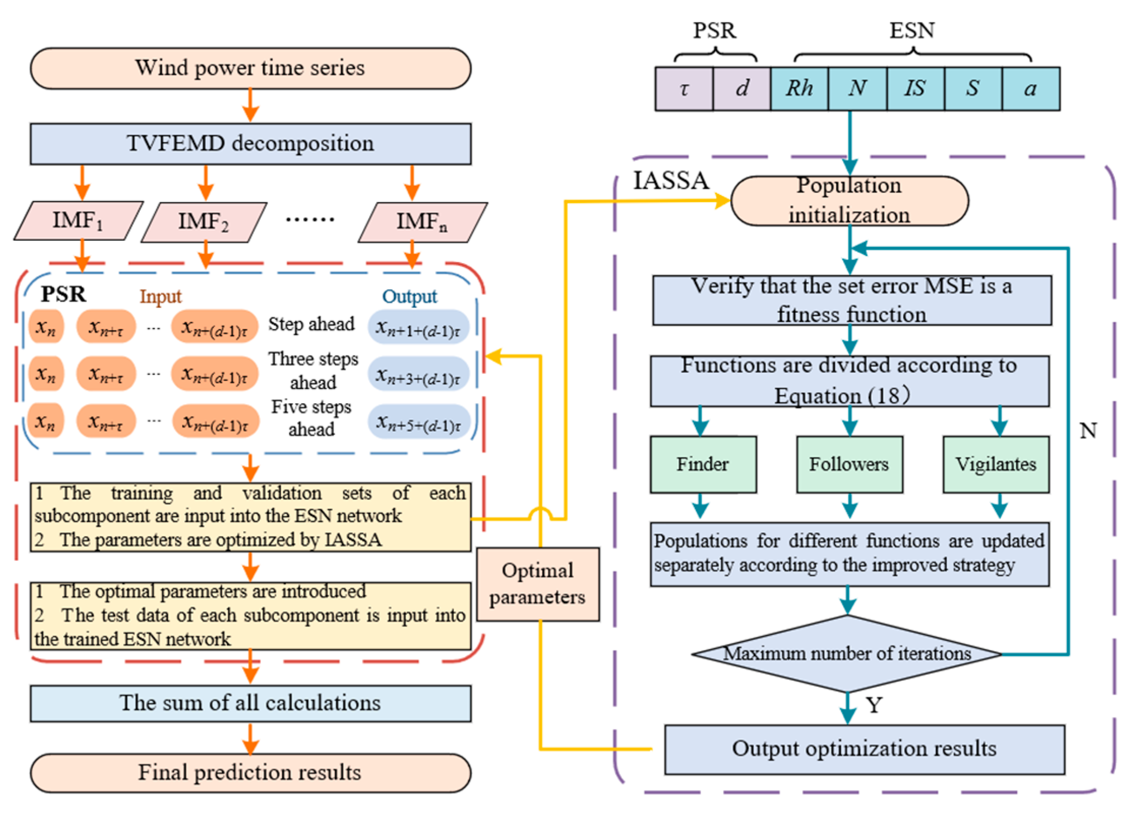
We developed a wind power hybrid prediction model by using TVFEMD, PSR, and ESN. To improve the prediction accuracy, the IASSA optimization algorithm was used to determine the optimal parameters of PSR and ESN simultaneously. The parameters τ and d in PSR and Rh, N, IS, and S in the ESN were encoded together in the IASSA. In addition, the root mean-square error (RMSE) was used as the fitness function to solve the parameters. The steps involved in the hybrid model are shown in Figure 3 and are described as follows:
(1)
Raw wind power data were collected.
(2)
The original wind power time series was divided into a series of subsequences by using TVFEMD.
(3)
All subsequences were converted into phase space matrices by using PSR and divided into the training set, validation set, and test set.
(4)
The ESN model was trained using the training set to verify that the RMSE of the set was the minimum, and all parameters in PSR and ESN were optimized synchronously using IASSA.
(5)
The optimized optimal parameters were introduced into PSR-ESN, and the test set was ran in order to obtain the prediction results of the subseries.
(6)
The prediction results of all subcomponents were accumulated to obtain the final wind power prediction results.

5. Case Analysis

The wind power generation data of the Irish energy system were used for experimental analysis, the wind power generation time was collected from 0:00 on 1 January 2020 to 0:00 on 16 January 2020, and the sampling interval of experimental data was 15 min, yielding a total of 1152 pieces of data.

5.1. Description of the Experiment

In order to verify the prediction performance of the proposed TVFEMD-ISSA-PSR-ESN model, the single models BPNN and LSTM, and the combined models SSA-ESN, EMD-SSA-PSR-ESN, and TVFEMD-SSA-PSR-ESN were compared. For the performance evaluation of the prediction models, three indicators were used: root mean-square error (RMSE), mean absolute error (MAE), and mean absolute proportional error (MAPE):
R M S E = 1 N i = 1 N Y i Y i * 2
M A E = 1 N i = 1 N Y i Y i *
M A P E = 1 N i = 1 N 100 × Y i Y i * Y i
For the model involved in the experiment, the B-spline interpolation n and bandwidth threshold ξ for TVFEMD decomposition were set as 26 and 0.3, respectively. The parameters, namely delay time, embedding dimension d, network update weight a, reserve pool connection matrix scaling parameter Rh, reserve pool node number N, input data scaling coefficient Win, and reserve pool sparsity S, were determined using the proposed IASSA and SSA optimization algorithms. Other parameters are presented in Table 4. In the experiment, the training set, validation set, and test set accounted for 60%, 15%, and 25% of all subsequences, respectively.

5.2. Data Decomposition and Normalization

After the TVFEMD decomposition of the original wind power data, seven subsequences were obtained and were recorded as IMF1–IMF7, as shown in Figure 4. In order to better train the law of subsequences, all subsequences were normalized separately. The normalization formula is:
y = y max y min · x x min x max x min + y min
where y is the normalized data; x is the original wind power data; xmax and xmin are, respectively, the maximum and minimum values of wind power; ymax and ymin are, respectively, the maximum and minimum values of the mapping space; and the mapped space is [−1, 1].

5.3. Prediction Results and Analysis

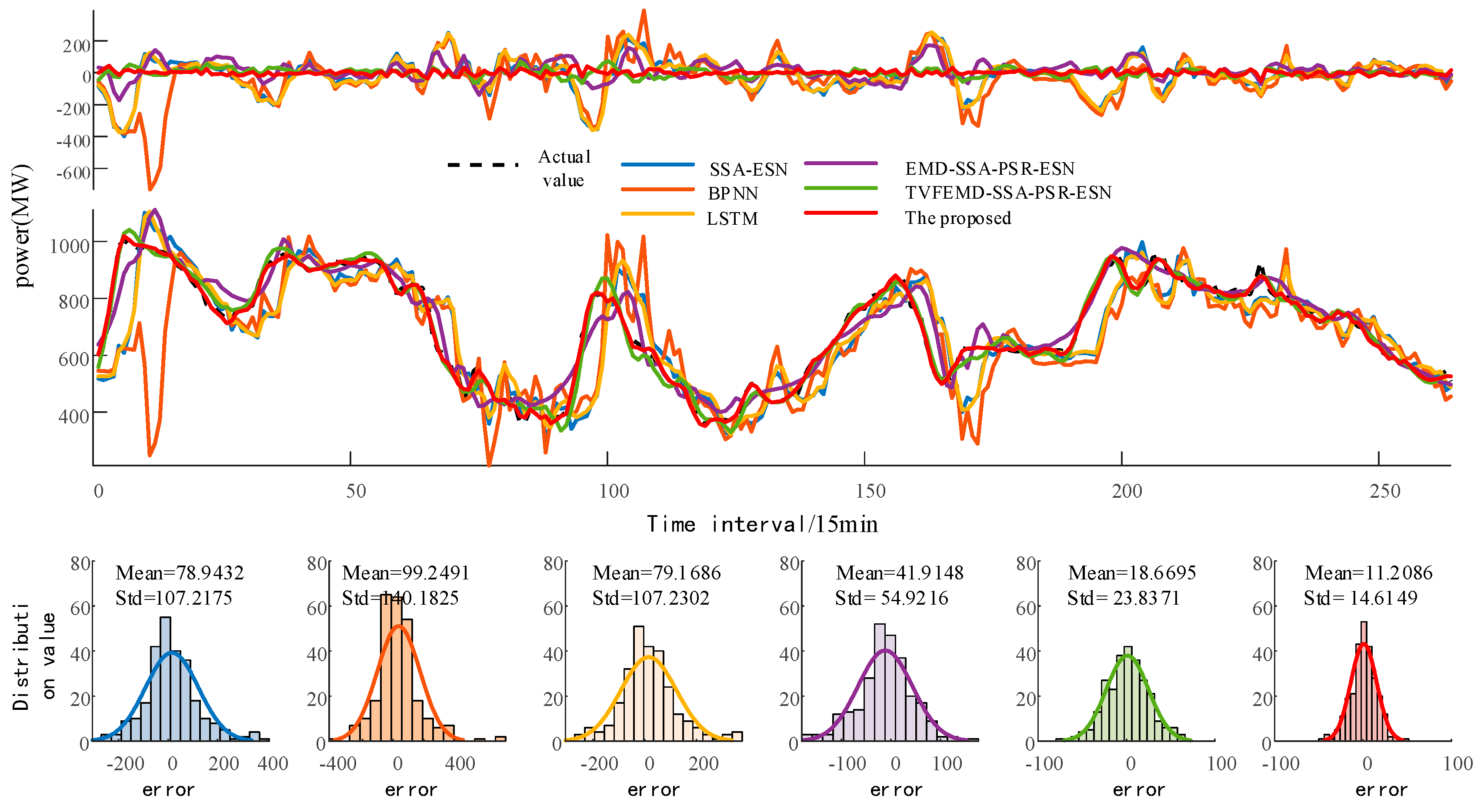
In this subsection, six experimental models are discussed in detail, and the prediction results are evaluated to demonstrate the validity of the proposed combined model. All experimental model prediction performance indicators, that is, RMSE, MAE, and MASE, including 1-, 3-, and 5-step-ahead predictions, are presented in Table 4, and the error radar chart is shown in Figure 5.
As can be seen from Table 5 and Figure 5, in the case of 1, 3, and 5 steps ahead, the proposed method predicted the wind power better, and the prediction error gradually increased with the increase in the number of prediction steps. A comparison of the evaluation indicators of different prediction models revealed the following points:
  • A comparison of the evaluation indicators RMSE, MAE, and MAPE of the SSA-ESN, BPNN, and LSTM models revealed that SSA-ESN had better prediction performance. In the 1-step, 3-step, and 5-step predictions, compared with BPNN and LSTM, the RMSE decreased by 3.2872 and 9.8666 (1 step), 7.8863 and 1.6156 (3 steps), and 30.1470 and 0.1169 (5 steps), respectively; the MAE decreased by 2.0291 and 11.6219 (1 step), 4.4120 and 1.2362 (3 steps), and 15.9460 and 0.5530 (5 steps); and the MAPE decreased by 0.3132 and 1.8950 (1 step), 0.6080 and 0.1861 (3 steps), and 2.2387 and 0.2191 (5 steps), respectively.
  • A comparative analysis of the models SSA-ESN, EMD-SSA-PSR–ESN, and TVFEMD-SSA-PSR–ESN revealed that the prediction performance of the model were greatly improved upon the addition of the signal decomposition method and PSR-ESN. The RMSE decreased by 17.8790 (1 step), 19.5499 (3 steps), and 32.8191 (5 steps); the MAE decreased by 12.0532 (1 step), 14.1699 (3 steps), and 24.0338 (5 steps); and the MAPE decreased by 1.9660 (1 step), 2.1109 (3 steps), and 3.5927 (5 steps).
  • Due to the drawbacks of the traditional SSA optimization methods, as well as PSR and ESN, requiring many parameters, SSA often falls into local optimal solutions. Therefore, in this study, the proposed IASSA was combined with PSR and ESN on the basis of TVFEMD to strengthen the prediction ability of the model through better parameter optimization performance. Comparing the TVFEMD-SSA-PSR-ESN model with the proposed model, the RMSE decreased by 1.2118 (1 step), 3.3657 (3 steps), and 9.3887 (5 steps); the MAE decreased by 0.9632, 2.4975, and 7.4163; and the MAPE decreased by 0.1258 (1 step), 0.3932 (3 steps), and 1.3014 (5 steps), respectively. Thus, the optimization performance of the IASSA not only has a certain effect on the classical test function but also exhibits good capacity to solve the actual parameter optimization problem.
In conclusion, the data analyses presented here highlight the effectiveness of the SSA-ESN model in terms of predictive performance when compared to BPNN and LSTM models. Furthermore, the inclusion of signal decomposition methods, PSR, and the proposed IASSA algorithm demonstrates significant improvements in the models’ predictive capabilities. These findings underscore the importance of selecting appropriate techniques and algorithms to optimize data analysis models for the achievement of enhanced performances and better results in real-world applications.
In order to verify the performance of the proposed method more intuitively, the experimental prediction effect was further visualized and analyzed. The error curves, fitting curves, and error distributions of the multistep prediction of the six models are shown in Figure 6, Figure 7, and Figure 8, respectively. To demonstrate the advantages of the proposed model more intuitively, the distribution value of the error was studied; the abscissa of the proposed method was found to be smaller, and its MAE and standard deviation were the smallest—3.2511 and 4.1478 (1 step), 7.5864 and 9.8941 (3 steps), and 11.2086 and 14.6149 (5 steps), respectively. This demonstrated the superiority of the proposed method.

6. Conclusions

In this paper, we proposed a hybrid model based on TVFEMD, PSR, ESN, and IASSA to predict short-term multistep wind power generation. In the proposed model, first, the wind power of the original time series is decomposed into multiple subcomponents by using TVFEMD, which effectively solves the problem of the difficult prediction of non-stationary signals. Next, the subcomponents are constructed by PSR to construct the output vectors of the prediction model, and the ESN is then used as the final prediction model to predict the data. Because PSR and ESN involve the adjustment of multiple parameters, the IASSA algorithm is used to optimize PSR and ESN parameters synchronously. Through a comprehensive experimental analysis of real wind power, the effectiveness of the proposed model is verified.
Based on the experimental results, the following conclusions can be drawn:
(1)
A comparison of the performance of EMD and TVFEMD decomposition of the original wind power time series revealed that TVFEMD, combined with the prediction model, yielded an improved prediction effect: the difference was expressed via number of steps, namely, 1 step, 3 steps, and 5 steps, and the effect was more obvious.
(2)
Compared with the original SSA, the proposed IASSA exhibited a better optimization performance in the classical test function and the actual prediction application. The accuracy was effectively improved in the three performance evaluations of root mean-square error (RMSE), mean absolute error (MAE) and mean absolute proportional error (MAPE).
(3)
Compared with six existing models, the experimental analysis of multistep prediction revealed that the proposed prediction model combining TVFEMD, PSR, ESN, and IASSA synchronous optimization strategies were able to effectively improve the prediction accuracy.
Based on the above three points, the combined prediction model proposed in this paper improved the accuracy of wind power research and provided a new feasible strategy for the multistep prediction of wind power.

Author Contributions

Conceptualization, C.T. and W.T.; methodology, W.T.; software, W.T.; validation, C.T., W.T. and L.Y.; formal analysis, C.T. and L.Y.; investigation, W.T.; resources, Y.S.; data curation, W.T.; writing—original draft preparation, W.T.; writing—review and editing, W.T.; visualization, Y.S.; supervision, C.T.; project administration, C.T.; funding acquisition, C.T. and Y.S. All authors have read and agreed to the published version of the manuscript.

Funding

This research was funded by National Natural Science Foundation of China, grant number “62273200”.

Institutional Review Board Statement

Not applicable.

Informed Consent Statement

Not applicable.

Data Availability Statement

The data used during the study are available from the first author by request.

Acknowledgments

We acknowledge the teacher for their help and the wind power data provided by the Irish energy system.

Conflicts of Interest

The authors declare no conflict of interest.

References

  1. Vahidzadeh, M.; Markfort, C.D. Modified power curves for prediction of power output of wind farms. Energies 2019, 12, 1805. [Google Scholar] [CrossRef] [Green Version]
  2. Yang, N.; Dong, Z.; Wu, L.; Zhang, L.; Shen, X.; Chen, D.; Zhu, B.; Liu, Y. A comprehensive review of security-constrained unit commitment. J. Mod. Power Syst. Clean Energy 2022, 10, 562–576. [Google Scholar] [CrossRef]
  3. Yang, N.; Qin, T.; Wu, L.; Huang, Y.; Huang, Y.; Xing, C.; Zhang, L.; Zhu, B. A multi-agent game based joint planning approach for electricity-gas integrated energy systems considering wind power uncertainty. Electr. Power Syst. Res. 2021, 204, 107673. [Google Scholar] [CrossRef]
  4. Xu, P.; Fu, W.; Lu, Q.; Zhang, S.; Wang, R.; Meng, J. Stability analysis of hydro-turbine governing system with sloping ceiling tailrace tunnel and upstream surge tank considering nonlinear hydro-turbine characteristics. Renew. Energy 2023, 210, 556–574. [Google Scholar] [CrossRef]
  5. Zhang, Y.; Wei, L.; Fu, W. Secondary frequency control strategy considering DoS attacks for MTDC sys-tem. Electr. Power Syst. Res. 2023, 214, 108888. [Google Scholar] [CrossRef]
  6. Zhang, Y.; Xie, X.; Fu, W. An Optimal Combining Attack Strategy Against Economic Dispatch of In-tegrated Energy System. IEEE Trans. Circuits Syst. II Express Briefs 2023, 70, 246–250. [Google Scholar]
  7. Ding, T.; Yang, M.; Yu, Y.; Si, Z.; Zhang, Q. Short-term Wind Power Integration Prediction Method Based on Error Correction. High Volt. Eng. 2022, 48, 488–496. [Google Scholar]
  8. Hu, W.; Zhang, X.; Li, Z.E. Short-term load forecasting based on an optimized VMD-mRMR-LSTM model. Power Syst. Protect. Control 2022, 50, 88–97. [Google Scholar]
  9. Fang, P.; Fu, W.; Wang, K.; Xiong, D.; Zhang, K. A compositive architecture coupling outlier correction, EWT, nonlinear Volterra multi-model fusion with multi-objective optimization for short-term wind speed forecasting. Appl. Energy 2022, 307, 118191. [Google Scholar]
  10. Hu, S.; Xiang, Y.; Shen, X.; Liu, J.; Liu, J.; Li, J. Wind power prediction model considering meteorological factor and spatial correlation of wind speed. Autom. Elec. Power Syst. 2021, 45, 28–36. [Google Scholar]
  11. Cheng, L.; Zang, H.; Xu, Y.; Wei, Z.; Sun, G. Augmented convolutional network for wind power prediction: A new recurrent architecture design with spatial-temporal image inputs. IEEE Trans. Ind. Inform. 2021, 17, 6981–6993. [Google Scholar] [CrossRef]
  12. Yang, M.; Dong, H. Short-term Wind Power Interval Prediction Based on Wind Speed of Numerical Weather Prediction and Monte Carlo Method. Power Syst. Autom. 2021, 45, 79–85. [Google Scholar]
  13. Liu, M.D.; Ding, L.; Bai, Y.L. Application of hybrid model based on empirical mode decomposition, novel recurrent neural networks and the ARIMA to wind speed prediction. Energy Convers. Manag. 2021, 233, 113917. [Google Scholar] [CrossRef]
  14. Dong, Y.; Ma, S.; Zhang, H.; Yang, G. Wind Power Prediction Based on Multi-class Autoregressive Moving Average Model with Logistic Function. J. Mod. Power Syst. Clean Energy 2022, 10, 1184–1193. [Google Scholar] [CrossRef]
  15. Wang, X.; Li, J.; Shao, L.; Liu, H.; Ren, L.; Zhu, L. Short-Term Wind Power Prediction by an Extreme Learning Machine Based on an Improved Hunter–Prey Optimization Algorithm. Sustainability 2023, 15, 991. [Google Scholar] [CrossRef]
  16. Tian, W.; Bao, Y.; Liu, W. Wind Power Forecasting by the BP Neural Network with the Support of Machine Learning. Math. Probl. Eng. 2022, 2022, 7952860. [Google Scholar] [CrossRef]
  17. van Heerden, L.; Vermeulen, H.; van Staden, C. Wind Power Forecasting using Hybrid Recurrent Neural Networks with Empirical Mode Decomposition. In Proceedings of the 2022 IEEE International Conference on Environment and Electrical Engineering and 2022 IEEE Industrial and Commercial Power Systems Europe (EEEIC/I&CPS Europe), Prague, Czech Republic, 28 June–1 July 2022; pp. 1–6. [Google Scholar] [CrossRef]
  18. Wang, D.; Cui, X.; Niu, D. Wind Power Forecasting Based on LSTM Improved by EMD-PCA-RF. Sustainability 2022, 14, 7307. [Google Scholar] [CrossRef]
  19. Fu, W.; Jiang, X.; Li, B.; Tan, C. Rolling bearing fault diagnosis based on 2D time-frequency images and data augmentation technique. Meas. Sci. Technol. 2023, 34, 045005. [Google Scholar] [CrossRef]
  20. Ding, M.; Zhou, H.; Xie, H.; Wu, M.; Nakanishi, Y.; Yokoyama, R. A gated recurrent unit neural networks based wind speed error correction model for short-term wind power forecasting. Neurocomputing 2019, 365, 54–61. [Google Scholar] [CrossRef]
  21. Ruiz-Aguilar, J.J.; Turias, I.; González-Enrique, J.; Urda, D.; Elizondo, D. A permutation entropy-based EMD–ANN forecasting ensemble approach for wind speed prediction. Neural Comput. Appl. 2021, 33, 2369–2391. [Google Scholar] [CrossRef]
  22. Zhang, C.; Ma, H.; Hua, L.; Sun, W.; Nazir, M.S.; Peng, T. An evolutionary deep learning model based on TVFEMD, improved sine cosine algorithm, CNN and BiLSTM for wind speed prediction. Energy 2022, 254, 124250. [Google Scholar] [CrossRef]
  23. Liu, Y.; Zhao, Q. Ultra-short-term power load forecasting based on cluster empirical mode decomposition of CNN-LSTM. Power Syst. Technol. 2021, 45, 4444–4451. [Google Scholar]
  24. Wang, R.; Li, C.; Fu, W.; Tang, G. Deep learning method based on gated recurrent unit and variational mode decomposition for short-term wind power interval prediction. IEEE Trans. Neural Netw. Learn. Syst. 2020, 31, 3814–3827. [Google Scholar] [CrossRef] [PubMed]
  25. Yang, N.; Yang, C.; Wu, L.; Shen, X.; Jia, J.; Li, Z.; Chen, D.; Zhu, B.; Liu, S. Intelligent data-driven decision-making method for dynamic multisequence: An E-seq2seq-based SCUC expert system. IEEE Trans. Ind. Inform. 2022, 18, 3126–3137. [Google Scholar] [CrossRef]
  26. Yang, N.; Yang, C.; Xing, C.; Ye, D.; Jia, J.; Chen, D.; Shen, X.; Huang, Y.; Zhang, L.; Zhu, B. Deep learning-based SCUC decision-making: An intelligent data-driven approach with self-learning capabilities. IET Gener. Transm. Distrib. 2022, 16, 629–640. [Google Scholar] [CrossRef]
  27. Hu, H.; Wang, L.; Tao, R. Wind speed forecasting based on variational mode decomposition and improved echo state network. Renew. Energy 2021, 164, 729–751. [Google Scholar] [CrossRef]
  28. Xu, M.; Wang, Y. Time series prediction based on improved differential evolution and echo state network. Chin. J. Autom. 2021, 47, 1589–1597. [Google Scholar]
  29. Wang, Z.; Wang, C.; Chen, L.; Li, G.; Gao, J. Photovoltaic power combined prediction based on ensemble empirical mode decomposition and deep learning. High Volt. Eng. 2022, 48, 4133–4142. [Google Scholar] [CrossRef]
  30. Li, L.L.; Liu, Z.F.; Tseng, M.L.; Jantarakolica, K.; Lim, M.K. Using enhanced crow search algorithm optimization-extreme learning machine model to forecast short-term wind power. Expert Syst. Appl. 2021, 184, 115579. [Google Scholar] [CrossRef]
  31. Samadianfard, S.; Hashemi, S.; Kargar, K.; Izadyar, M.; Mostafaeipour, A.; Mosavi, A.; Nabipour, N.; Shamshirband, S. Wind speed prediction using a hybrid model of the multi-layer perceptron and whale optimization algorithm. Energy Rep. 2020, 6, 1147–1159. [Google Scholar] [CrossRef]
  32. Du, M. Improving LSTM Neural Networks for Better Short-Term Wind Power Predictions. In Proceedings of the 2019 IEEE 2nd International Conference on Renewable Energy and Power Engineering (REPE), Toronto, ON, Canada, 4–6 November 2019; pp. 105–109. [Google Scholar] [CrossRef] [Green Version]
  33. Xiong, D.; Fu, W.; Wang, K.; Fang, P.; Chen, T.; Zou, F. A blended approach incorporating TVFEMD, PSR, NNCT-based multi-model fusion and hierarchy-based merged optimization algorithm for multi-step wind speed prediction. Energy Convers. Manag. 2021, 230, 113680. [Google Scholar] [CrossRef]
  34. Fu, W.; Zhang, K.; Wang, K.; Wen, B.; Fang, P.; Zou, F. A hybrid approach for multi-step wind speed forecasting based on two-layer decomposition, improved hybrid DE-HHO optimization and KELM. Renew. Energy 2021, 164, 211–229. [Google Scholar] [CrossRef]
  35. Ju, Y.; Qi, L.; Liu, S. Short-term wind power forecasting based on improved crow search algorithm and ESN neural network. Power Syst. Protect. Control 2019, 47, 58–64. [Google Scholar]
  36. Xue, J.; Shen, B. A novel swarm intelligence optimization approach: Sparrow search algorithm. Syst. Sci. Control Eng. 2020, 8, 22–34. [Google Scholar] [CrossRef]
  37. Ma, J.; Hao, Z.; Sun, W. Enhancing sparrow search algorithm via multi-strategies for continuous optimization problems. Inf. Process. Manag. 2022, 59, 102854. [Google Scholar] [CrossRef]
  38. Mirjalili, S.; Lewis, A. The whale optimization algorithm. Adv. Eng. Softw. 2016, 95, 51–67. [Google Scholar] [CrossRef]
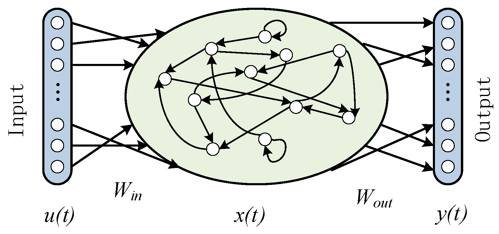
Figure 1. Structure of the ESN.
Sustainability 15 09107 g001
Figure 2. Convergence effect of different algorithms.
Sustainability 15 09107 g002
Figure 3. Flowchart of the wind power prediction model.
Sustainability 15 09107 g003
Figure 4. Decomposition results of wind power data.
Sustainability 15 09107 g004
Figure 5. Error radar charts for different models in multistep prediction: (a) RMSE; (b) MAE; (c) MAPE.
Sustainability 15 09107 g005
Figure 6. One-step-ahead prediction results of different models.
Sustainability 15 09107 g006
Figure 7. Three-step-ahead prediction results of different models.
Sustainability 15 09107 g007
Figure 8. Five-step ahead prediction results of all models.
Sustainability 15 09107 g008
Table 1. Single-peak and multipeak test functions.
FunctionDimensionOptimal Value
F 1 ( x ) = i = 1 n x i 2 300
F 2 ( x ) = i = 1 n x i + i = 1 n x i 300
F 3 ( x ) = i = 1 n j = 1 i x j 2 300
F 4 ( x ) = i = 1 n x i sin x i 300
F 5 ( x ) = 20 exp 0.2 1 n i = 1 n x i 2 exp 1 n i = 1 n cos 2 π x i + 20 + e 300
F 6 ( x ) = 0.1 sin 2 3 π x 1 + i = 1 n x i 1 2 1 + sin 2 3 π x i + 1 + x n 1 2 1 + sin 2 2 π x n + i = 1 n u x i , 5 , 100 , 4 300
Table 2. Test function optimization results.
GWOPSOSSAIASSA
AVESTDAVESTDAVESTDAVESTD
F16.440 × 10−94.361 × 10−90.26020.1312.607 × 10−67.343 × 10−61.459 × 10−585.459 × 10−58
F26.493 × 10−63.116 × 10−61.2430.3980.00460.00471.967 × 10−305.021 × 10⁻³⁰
F37.00210.1134.3701.4733.354 × 10−45.799 × 10−46.249 × 10−423.410 × 10−41
F4−5.985 × 1039.992−3.351 × 1034.544−7.712 × 1038.516−7.722 × 1028.395
F50.00870.0165.7892.0738.297 × 10−82.712 × 10−700
F632.35436.0922.508 × 1051.099 × 1051.654 × 10−52.941 × 10−51.544 × 10−55.064 × 10⁻⁶
Table 3. The convergence time of different algorithms.
F1
(s)
F2
(s)
F3
(s)
F4
(s)
F5
(s)
F6
(s)
IASSA0.0168750.0176370.0436070.0196180.019440.33775
SSA0.0178710.0181490.0441310.0229350.0204010.40221
GWO0.0175660.0181480.0384410.0218970.0190670.32584
PSO0.00765620.0077210.0281810.0136130.0107780.39815
Table 4. Parameter settings of all experimental methods.
MethodSearch MethodParameterParameter Methods
SSA/
IASSA
PresetPopulation size30
PresetNumber of iterations100
PresetProportion of discoverers0.2/[0.2, 0.8]
ESNSSA/IASSAThe number of reserve pool nodes is N[20, 500]
SSA/IASSASparseness degree S[0.01, 0.1]
SSA/IASSAReserve pool connection matrix scaling parameter Rh[0.01, 1]
SSA/IASSAEnter the data scaling factor IS[0.01, 1]
SSA/IASSAUpdate weight a[0.01, 1]
LSTM/
BPNN
PresetNumber of hidden layers1
PresetThe number of hidden layer nodes50
TVFEMDPresetB-spline interpolation n26
PresetBandwidth threshold ξ0.3
PSRSSA/IASSAEmbedding dimension D[1, 10]
SSA/IASSADelay time τ[1, 50]
Table 5. Multistep prediction errors of different models.
Model1 Step Ahead3 Step Ahead5 Step Ahead
RMSEMAEMAPERMSEMAEMAPERMSEMAEMAPE
(MW)(MW)(%)(MW)(MW)(%)(MW)(MW)(%)
SSA-ESN29.589920.19823.452366.640846.68747.859298.309070.940511.7082
BPNN32.877122.22733.765574.527151.09948.4672128.456086.886513.9469
LSTM39.456531.82015.347368.256447.92368.045398.425971.493511.9273
EMD-SSA-PSR-ESN22.972916.00402.596132.114723.62093.659756.019941.91486.5519
TVFEMD-SSA-PSR-ESN5.09393.95080.630112.56489.45101.548823.200817.88102.9592
This article method3.88212.98760.50439.19916.95351.155613.812110.46471.6578
Disclaimer/Publisher’s Note: The statements, opinions and data contained in all publications are solely those of the individual author(s) and contributor(s) and not of MDPI and/or the editor(s). MDPI and/or the editor(s) disclaim responsibility for any injury to people or property resulting from any ideas, methods, instructions or products referred to in the content.