An Efficient Approach to Monocular Depth Estimation for Autonomous Vehicle Perception Systems

Abstract

Depth estimation is critical for autonomous vehicles (AVs) to perceive their surrounding environment. However, the majority of current approaches rely on costly sensors, making wide-scale deployment or integration with present-day transportation difficult. This issue highlights the camera as the most affordable and readily available sensor for AVs. To overcome this limitation, this paper uses monocular depth estimation as a low-cost, data-driven strategy for approximating depth from an RGB image. To achieve low complexity, we approximate the distance of vehicles within the frontal view in two stages: firstly, the YOLOv7 algorithm is utilized to detect vehicles and their front and rear lights; secondly, a nonlinear model maps this detection to the corresponding radial depth information. It is also demonstrated how the attention mechanism can be used to enhance detection precision. Our simulation results show an excellent blend of accuracy and speed, with the mean squared error converging to 0.1. The results of defined distance metrics on the KITTI dataset show that our approach is highly competitive with existing models and outperforms current state-of-the-art approaches that only use the detected vehicle’s height to determine depth.

1. Introduction

Autonomous vehicles have the potential to enhance road efficiency, minimize traffic accidents, and reduce our environmental footprint. However, the successful practical reality perspective of the fully autonomous vehicle is based on the reliability of their perception pillar. Accurate distance estimation is critical in path planning and avoiding collisions with vehicles, pedestrians, and objects in the surrounding environment in the context of self-driving perception tasks. Rear-end collisions are a significant cause of traffic accidents [1,2] and can often be prevented by maintaining an appropriate following distance to the vehicle in front. Distance estimation is thus an essential issue for ensuring the safety of autonomous vehicles, but it is also a challenging problem to solve; the proposed solutions must be efficient for real-time applications while being cost-effective for widespread industry deployment. There are three primary categories for distance measurement techniques: active sensor-based, passive vision-based, and fusion-based. Active sensors, including ultrasonic and light detection and ranging (LiDAR), operate by emitting a sound or laser pulse, calculating the time it takes for the pulse to be reflected back to the sensor’s pulse detector, and then using this information to calculate the distance [3]. Ultrasonic sensors are inexpensive, inaccurate devices that are suitable for basic short-range applications [4,5], whereas LiDAR systems are accurate but heavy and expensive [6,7,8], making them unsuitable for industrial deployment [9].

The transmission of signals from sensors located in other vehicles can exert a significant impact on the performance of active sensors [9,10]. Additionally, these systems may encounter challenges in accurately distinguishing between different objects located in the frontal view. Fusion-based methods can provide more reliable measurement results because they combine the advantages of both prior methods. However, they are more complex to implement because they require the integration of multiple sensor types. Passive vision-based methods are generally less expensive and easier to implement because they rely only on the camera and do not require additional equipment [11]. Compared to sonar and LiDAR, a camera is able to see further [12] and detect the edges and details of objects. This ultimately provides an advantage in terms of situational awareness, allowing for a more detailed view of the environment. They can also be easily integrated into existing systems, allowing for rapid and cost-effective deployment in various scenarios.

Passive sensor-based techniques are highly favored in current studies, largely due to extensive adoption of image sensors. The stereo vision technique, which is inspired by the human visual perception mechanism, incorporates multi-view geometry and generates depth information for every pixel via an error-prone matching process between stereo image pairs [5,7,13]. Nevertheless, this approach can prove to be inefficient due to the complexity of the calibration process and the high cost and weight associated with high-quality stereo cameras [5,7,14,15].

Another ideal solution is to use a monocular camera to estimate the distance to an object based on geometric attributes within two-dimensional (2D) images and camera characteristics. Kim and Cho [16] estimated inter-vehicle distance using the relative position of the camera from the front vehicle and the width of the front car. One of the main drawbacks of the Kim and Cho [16] method is that it ignores the actual size of the vehicles. Liu et al. [10] addressed this issue by converting an image into a bird’s eye view and using inverse perspective mapping to estimate the distance between vehicles. Despite this improvement, inaccuracies in determining camera parameters and image brightness could potentially introduce errors into their measurements.

Recently, deep learning-based monocular distance estimation has received more attention [17,18,19,20]. By employing a monocular camera, Hu et al. [18] conducted a study on object tracking and detection, where they focused on obtaining valuable data about the distances between objects to enhance the performance of the tracker. Their research aimed to improve the efficiency of a faster R-CNN model by incorporating estimations of both the angle and distance of objects. Another study [21] employed a lightweight MTCNN for license plate detection and utilized an MLP to model the perspective relationship between license plate dimensions and depth. Although this approach primarily depends on license plate information, it can be useful as an auxiliary method for depth estimation. Ref. [22] employed the popular object-detection framework, YOLOv3, to detect bounding boxes and their coordinates. The distances between objects were then calculated analytically. However, this method did not consider the relationship between the object’s size and its distance, which can lead to inaccurate distance estimations. To overcome this limitation, DisNet [23] combined YOLOv3 with a fully connected neural network that was separately trained on the basis of the predictions acquired from YOLO. The network generated more accurate distances by considering the object’s size and distance relationship. However, this approach requires additional training and computational resources. Chen et al. [24] developed Monodepth [25], combined with YOLOv3, to estimate the distances between objects. Monodepth generated a disparity map using visual data from two cameras, which was then used to estimate the distance of the object from a single camera. The estimated distance was then injected into the predicted bounding boxes of YOLO, resulting in accurate distance estimations. However, this method requires additional cameras and complex training. Strbac et al. [26] employed two YOLOv3 detectors and two cameras to estimate distances using the stereoscopic principle. This approach provided accurate distance estimations, but the use of two detectors increased computation time, and distance measurements may not be possible when an object is detected by only one detector.

There has been an increasing amount of research on estimating distance using a monocular image in recent years, especially in the areas of inter-vehicle distance estimation [27] and advanced driver assistance systems (ADASs) [5]. Some studies have concentrated on using the bounding box’s height to form the object’s feature vector, but Tousi et al. [28] argued that relying solely on the height of a car in an image may lead to more errors. To reduce sensitivity to errors caused by the placement of bounding boxes, they proposed an alternative approach that is less susceptible to such errors.

This paper presents an efficient method for estimating depth from a monocular image using vehicle lights, while also offering a practical way to achieve a tradeoff between speed and accuracy for real-time distance estimation in an autonomous vehicle. To this end, various alternative methods for detecting objects in images have been investigated, and among these, “You Only Look Once” (YOLO) [29], has demonstrated the highest effectiveness. YOLOv7 significantly improves real-time object detection performance while lowering overhead [30]. In our approach, the YOLOv7 network was employed to train a model for detecting vehicle’s lights. For our data-driven method, we created a dataset of car lights with object detection frames, comprising 4700 cars and their corresponding labels. Furthermore, this study utilizes an enhanced attention mechanism, the YOLOv7-CBAM algorithm, which integrates three CBAM modules into the YOLOv7 backbone network. This modification enhances the precision of our network’s detection capabilities. In order to obtain the required data, multiple driving scenes were simulated on CARLA. After the detection step, by mapping the output of the detection and recognition network to the estimated depth value through MLP, a more accurate estimation of depth can be achieved.

Section 2 provides the fundamental background required to understand the distance estimation problem and how to approach it, and outlines our specific approach. Section 3 explains the details of the training process and the results that were obtained, and summarizes the key findings from the experiments. Section 4 concludes with a summary of the results.

2. Materials and Methods

2.1. Deep-Learning-Based Object Detection Approaches

Object detection is a difficult and essential task in computer vision which entails accurately identifying objects in images or videos by predicting their classification probability and localizing them using bounding boxes. Recent advancements in deep learning have enabled significant progress in identifying objects in autonomous driving scenes, such as detecting traffic lights [31,32,33], road signs [34,35], pedestrians [36,37], and vehicles [38,39,40].

There are two main approaches to achieve deep learning object detection: two-stage and one-stage methods, which are commonly used in cutting-edge object detection networks. In two-stage methods such as OverFeat [41] and R-CNN [42], a selective search or a similar algorithm generates region proposals, then classifies and refines them by a separate detection network. Recent methods such as SPPnet [43] and Fast-RCNN [44] have improved the speed and efficiency of the two-stage detectors by using global feature maps generated by a larger CNN applied to the entire input image with the aim of directly obtaining regional features. It should be noted that these methods frequently use popular CNN architectures as base models, such as VGG [45], ResNet [46], and GoogLeNet [47].

Faster R-CNN [48] is a two-stage approach that significantly improves the accuracy of object detection by incorporating the Region Proposal Network (RPN) as a network component. The RPN is a fully connected network that generates region proposals by sliding over high-level CNN feature maps, which are then passed to the network’s subsequent stages for classification and bounding box regression. By integrating the RPN into the network, Faster R-CNN can generate region proposals more accurately and efficiently than previous methods. However, the computational complexity of Faster R-CNN makes it unsuitable for real-time applications, where detection speed is critical. Thus, attention has been directed to You Only Look Once (YOLO) [29].

YOLO utilizes a one-stage detection approach that combines the entire object detection process in a single architecture. Unlike Faster R-CNN, YOLO does not rely on an RPN (Region Proposal Network). Instead, it utilizes a single convolutional neural network to simultaneously predict object classes and bounding boxes for all objects in the image.

The architecture of YOLO comprises two parts, namely, the extractor and the detector. The extractor, represented by the Darknet-53 backbone or other backbones, aims to extract features from the input image [29]. The detector takes the features from the extractor and decodes them on multiple scales to predict object classes and bounding boxes for each cell in the output grids. This allows YOLO to perform object detection in real time with high accuracy [29].

The one-stage detection approach of YOLO is a more straightforward and efficient architecture compared to the two-stage object detection approaches. This makes it more suitable for real-world applications, including autonomous vehicles.

2.2. YOLOv7

YOLOv7 [30] model is a highly effective real-time object detection solution that enhances accuracy without increasing inference overhead. In benchmarks, YOLOv7 has demonstrated the ability to reduce 40% of parameters and 50% of computation in comparison to the most advanced real-time object detectors. In the study [30], the performance of YOLOv7 was evaluated against prior YOLO versions (YOLOv4 [49], YOLOv5 [50]) and YOLO-R [51], using the same training parameters as baselines. Based on the findings of the study [30], YOLOv7 has demonstrated superior performance in terms of average precision (AP) compared to all previous object detectors while maintaining impressive frame rates ranging from 5 to 160 frames per second. Therefore, YOLOv7 emerges as the leading choice for efficient and precise object detection tasks, offering the best balance between speed and accuracy. In this study, we trained the YOLOv7 model using our prepared dataset, excluding any additional image datasets or pre-trained weights for the model. YOLOv7 backbones, such as Scaled YOLOv4 [49], do not utilize Image Net pre-trained backbones (such as YOLOv3).

Compared to YOLOv4, YOLOv7 decreases the number of parameters by 75%, requires 36% less computation, and achieves an AP (average precision) score that is 1.5% higher. On the COCO dataset, the YOLOv7 real-time model obtains a 13.7% higher AP (43.1% AP) than the earlier most-accurate YOLOv6 model (56.8% AP) [30].

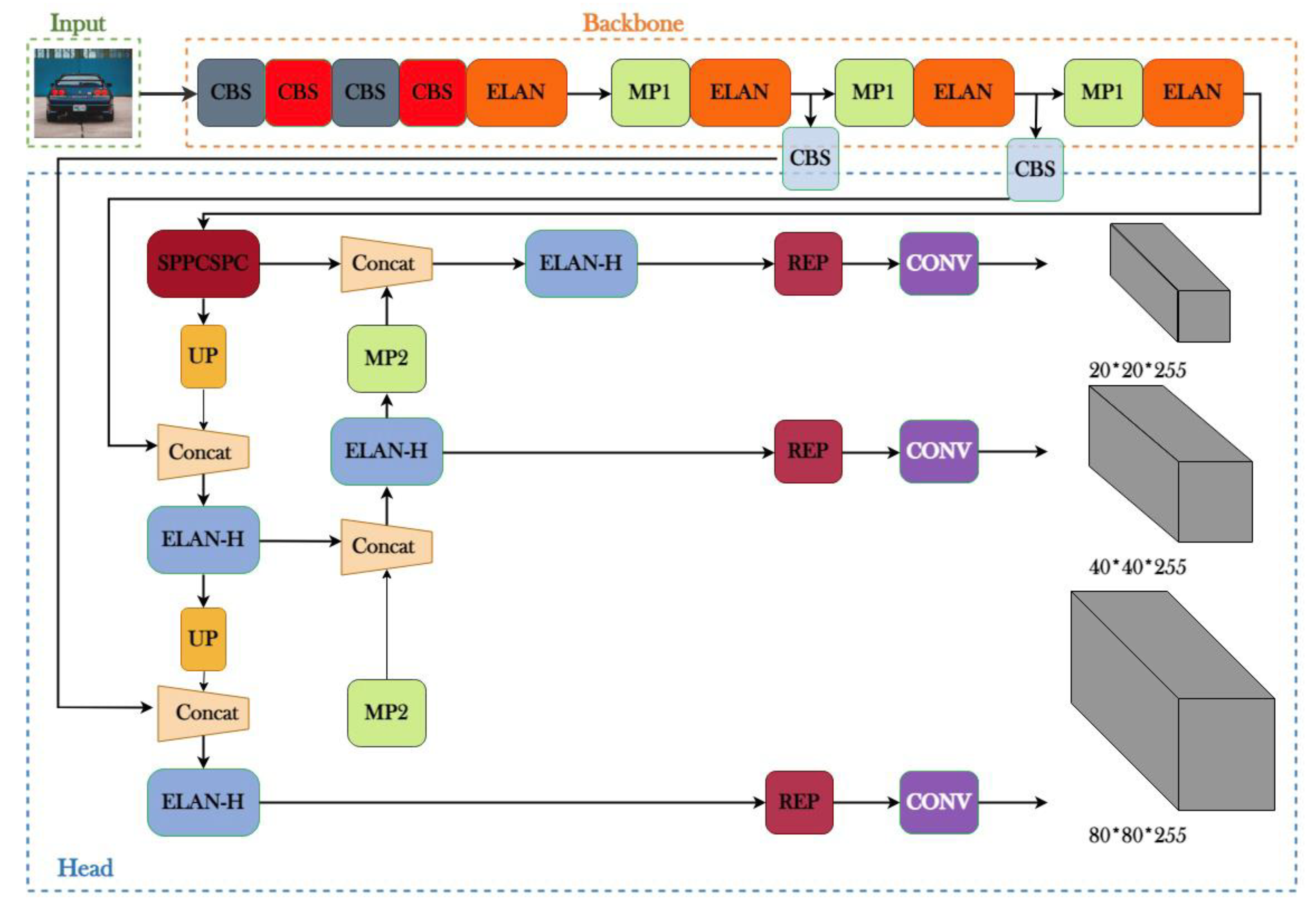
2.2.1. The YOLOv7 Architecture

The YOLOv7 architecture is an extension of previous designs such as YOLOv4 and YOLO-R. At its core, the YOLOv7 backbone utilizes the E-ELAN (Extended Efficient Layer Aggregation Network) computing block. This architecture improves the model’s learning capabilities through the “expand, shuffle, merge cardinality” method, which increases network learning accuracy without losing the original gradient track. The YOLOv7 network architecture diagram comprises four general modules, namely, the input terminal, backbone, head, and prediction. In addition, it has five basic components: CBS, MP, ELAN, ELAN-H, and SPPCSPC. Figure 1 provides an illustration of the YOLOv7 architecture, which can be divided into three main parts: input, backbone, and head.

During feature extraction, the backbone layer uses a combination of BConv layers, E-ELAN layers, and MPConv layers in an alternating pattern to progressively decrease the aspect ratio, double the channels, and extract relevant features. The head layer is responsible for prediction and comprises various layers, such as SPPCSPC layers, multiple BConv layers, MPConv layers, several Concat layers, and a RepVGG block layer, which generates three heads.

Once the head layer produces three feature maps, three unprocessed predictions of varying sizes are generated using the three REP and Conv layers.

2.2.2. Scaling of the YOLOv7 Compound Model

YOLOv7 introduces a novel compound model scaling technique that allows for the preservation of the model’s original characteristics while achieving the best arrangement. As an example, scaling a computational block’s depth factor alters its output channel, while the transition layers are scaled using the same width factor.

2.2.3. Re-Parametrized Convolution

The design of YOLOv7 re-parameterized convolution without identity connection employs RepConv (RepConvN). While RepConv has shown excellent performance in VGG architectures, its use in ResNet or DenseNet results in considerable accuracy loss.

2.2.4. Auxiliary Coarse, Lead Loss Fine

The YOLOv7 architecture is composed of three main components: the backbone, neck, and head. The head is responsible for the model predictions, and YOLOv7 allows for multiple heads due to its inspiration from deep supervision training. The lead head produces the final output, while the auxiliary head helps train intermediary layers.

Furthermore, a label assigner mechanism was added in order to enhance the deep network training. This mechanism considers the ground truth and the prediction results of the network prior to assigning soft labels. Contrary to the traditional assignment of labels, which is only dependent on the ground truth so as to generate hard labels on the basis of the prescribed rules, optimization and computation methods are employed by the dependable soft labels that consider the distribution and reliability of prediction outputs besides the ground truth.

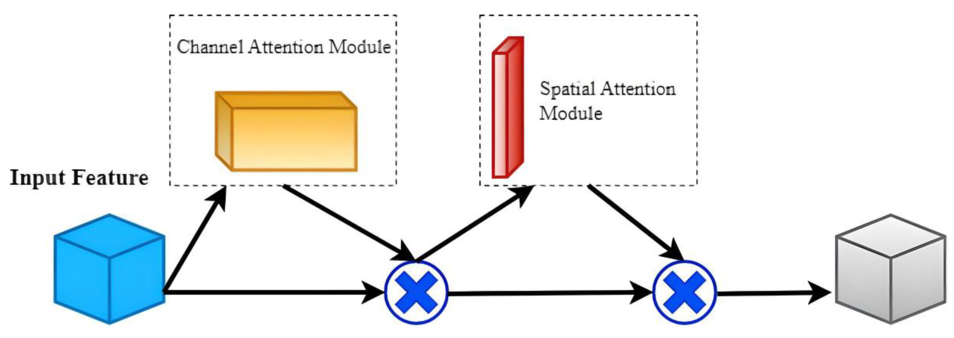
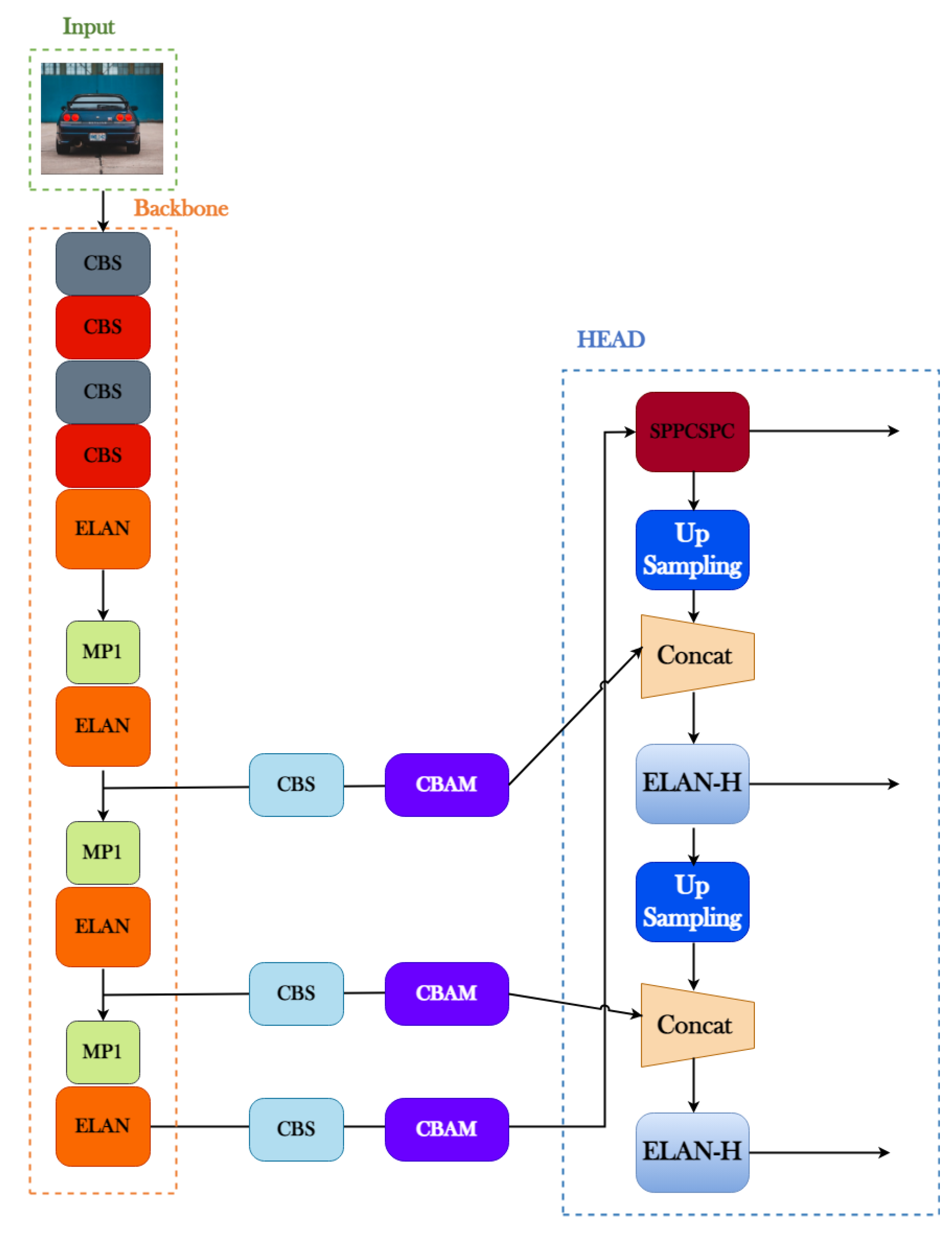
2.3. Integrating Attention Mechanism for Enhanced YOLOv7 Object Detection

The attention mechanism is a widely used technique in machine learning tasks that enables models to focus on the most relevant elements of input data while ignoring irrelevant parts [52]. This is achieved by assigning different weights to different parts of the input. In computer vision, the attention mechanism has been successfully applied to highlight critical features of the input, such as pixel attention, channel attention, and multi-order attention. These features help the model to identify important patterns and make more accurate predictions [43].

One of the most effective attention mechanism modules in computer vision is the Channel and Spatial Attention Module (CBAM) [53]. As shown Figure 2, CBAM is a lightweight attention module that includes a spatial attention module (SAM) and a channel attention module (CAM). CAM helps the network to identify the most important channels to become more focused on the meaningful area of the image, while SAM enables the network to focus on positions with contextual information about the entire image [54,55].

Figure 3 shows the integration of the CBAM module into the YOLOv7 architecture; the purpose of this module is to enhance the feature extraction capability of the network [30,53]. However, a previous study [56] indicated that adding the attention mechanism into the backbone network of YOLOv7 can lead to prediction inaccuracy due to the destruction of some of the backbone network’s original weights. Therefore, it is preferable to integrate the attention mechanism into the feature network extraction improvement section to prevent such errors. As a result, our approach effectively improves the network’s feature extraction abilities without compromising its primary features. This method holds promise for advancing the accuracy and reliability of object detection systems.

2.4. CARLA

In our research, we used Car Learning to Act (CARLA) [57], which is an open-source simulator developed for research on self-driving cars. CARLA operates as a server–client system, in which the client application programming interface (API) is developed using Python, and the server simulates and renders scenes. This simulator has a high degree of realism and accuracy, with accurate 3D models and detailed textures that can be used to simulate real-world scenarios. It also has a number of sensors, such as cameras and LiDAR. The environment simulation provided by CARLA [57] is incredibly detailed, allowing users to control the weather conditions, illumination, and the number and type of vehicles and pedestrians; it also provides RGB cameras which can be positioned and adjusted according to the user’s needs. The environment also includes a complex urban layout with intersections, roundabouts, and traffic lights that simulate a realistic driving experience for autonomous vehicles.

2.5. Preparation of Dataset

The first stage of this study involves identifying and detecting vehicles and their lights. To ensure proper training of the neural network and to achieve acceptable speed and accuracy in object detection, it is essential to have sufficient diversity in the dataset. To this end, Microsoft developed the COCO dataset [58], which contains 328,000 images labeled with objects from 91 different classes. However, there is no vehicle light class in the original COCO dataset [58]. To address this issue, we followed a two-step procedure. First, we selected the desired images from the original dataset, which included car, truck, and bus classes. Second, we labeled all lights on cars to create two new classes: front light and rear light. The resulting dataset consisted of 4700 images for training and 2100 images for validation, including road vehicles, front lights, and rear lights.

To enhance our model’s ability to accurately identify images from diverse environments, we employed data augmentation techniques to make modifications at the pixel level, including both photometric and geometric distortions. In order to address photometric distortions, we made adjustments to different aspects of the image, including Hue (−25° to +25°), Saturation (−23% to +23%), Brightness (−41% to +41%), Exposure (−27% to +27%), Blur (up to 2 pixels), and Noise (up to 5% of pixels). Additionally, we applied Horizontal and Vertical flipping and Rotation (−15° to +15°) to address geometric distortions. The primary aim of these modifications was to improve the diversity of the training data, thereby allowing the model to learn from a broader range of image conditions and to become more robust.

In preparing our car lights dataset, we focused on refining the model’s performance by adjusting the strength of photometric distortions, particularly in regard to the hue and saturation of the image. This approach enabled our model to better generalize to new and previously unseen data, which is crucial in achieving high performance in real-world scenarios. Furthermore, this method resulted in improved model performance without any additional computational cost during model inference.

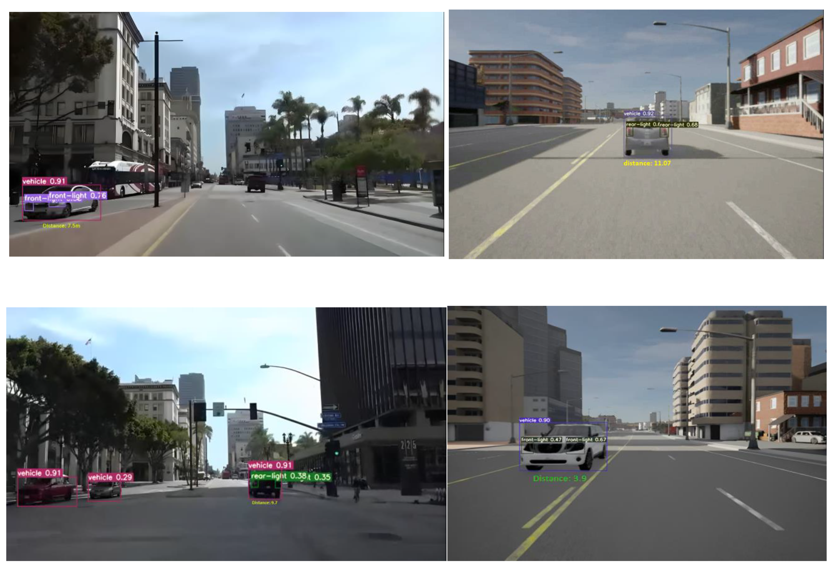
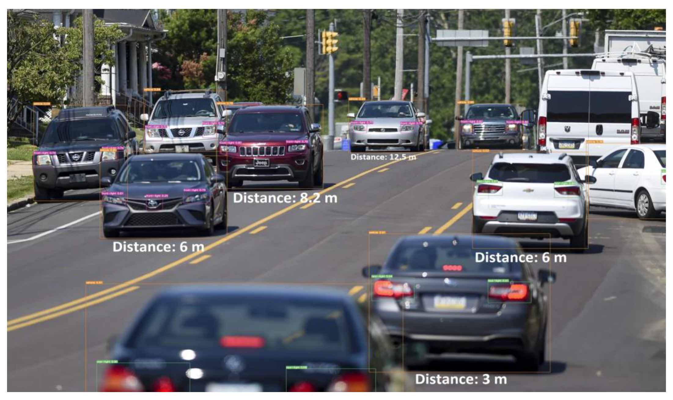
2.6. Intended Model

The height of the bounding box provides a good indication of the actual size of the object in the image, which in turn gives an estimate of the depth of the object in the scene. This is due to the fact that the objects situated further away seem smaller in the image compared to the ones situated closer. From another perspective, car width has much fewer variations, and therefore, it can serve as an appropriate parameter in the process of the prediction of depth. The object height in the image is highly dependent on the camera’s distance to it; however, the object width is less dependent. Nonetheless, such a technique is problematic because in cases that a car is at an angle instead of being directly in front of the camera, this technique does not function accurately, i.e., the detection bounding box has a greater width compared to the width of the car in the image. This is attributable to the limited field of view (FOV) of the camera, and, as a result, the objects situated farther away can hardly be observed in the image; therefore, the bounding box width cannot represent the car width accurately. According to [59], the orientation of the object components in an image conveys useful information about the depth of the objects. The distance between rear lights is approximately the same as the car width in the image. The car orientation in the image can be inferred through the measurement of the relative distances between the center of the rear lights and the center of the car bounding box. This provides extra information about its depth. Even though another car may occlude the light of the desired car in a number of cases, it is noteworthy that the distance to the nearest vehicle assumes greater importance as compared to the partially occluded ones.

In addition, when one rear light is occluded, the other one can still convey adequate data in order to determine the distance between the two lights accurately and, thereby, the width of the car plays a significant role in determining the orientation of vehicles. Additionally, occlusion effects can be reduced by tracking car lights. This is, in particular, advantageous in circumstances in which a number of cars are close together or when the car is occluded partially [60]. In such cases, it may present invaluable visual cues and reliable measurements.

The model proposed in this study, as shown in Figure 4, includes two separate parts for the depth estimation:

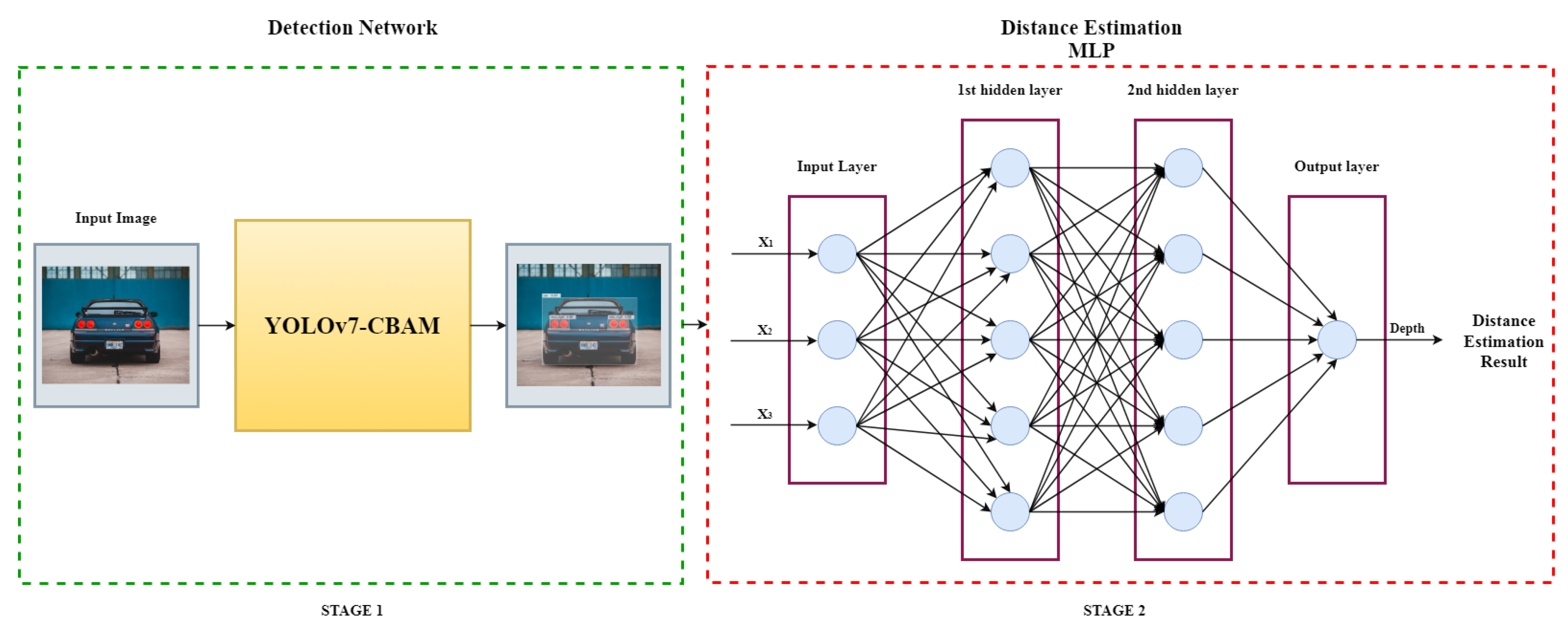
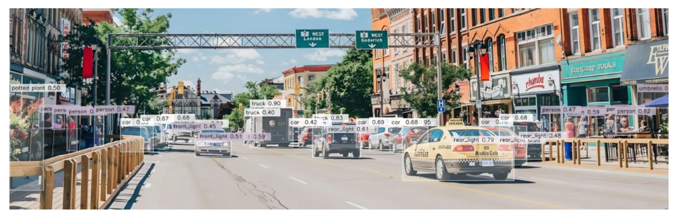
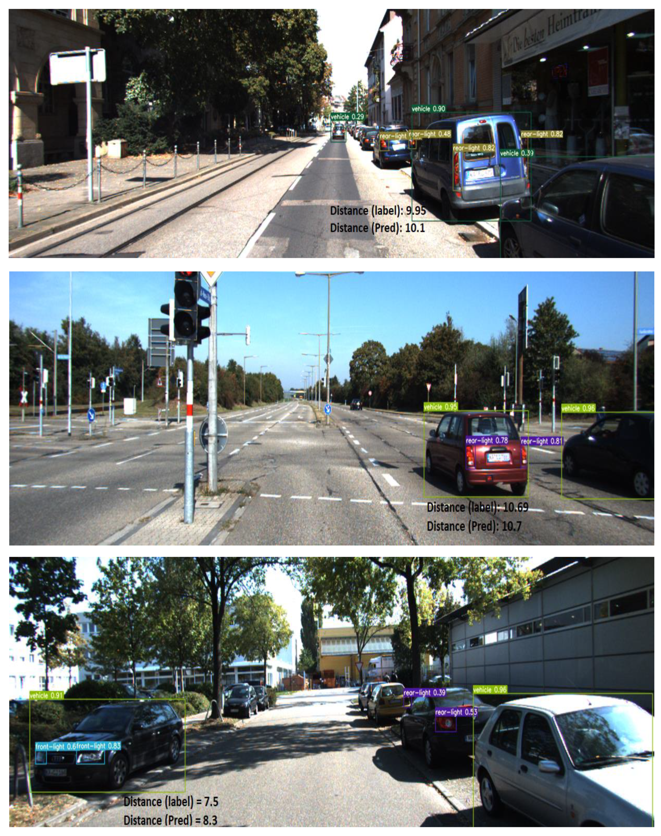
• Stage1: Detecting and recognizing the vehicle and its lights in the image.
• Stage2: The second part of the proposed approach to estimating vehicle depth, as shown in Figure 4, used MLP to map the information from the detection and recognition network to the estimated depth value.

According to the proposed diagram represented in Figure 4, since the first stage of this study requires recognizing and detecting vehicles and their lights, the network used for object detection must have satisfactory speed and accuracy. In most cases, focusing on increased accuracy minimizes the speed of object detection and thus weakens the network’s real-time performance. On the other hand, focusing too much on the recognition speed reduces the network’s accuracy. In the case of autonomous vehicles, failure to identify objects such as pedestrians or other vehicles can cause irreversible damage. Another notable issue is that a network may perform very successfully in object classification but not perform well in highly dynamic scenes. At the same time, a high processing speed is required for fast and proper vehicle reaction.

The detection network used in this study is the seventh version of the YOLO (YOLOv7) network. YOLOv7 [30] makes a good tradeoff between detection speed and accuracy. A study on depth detection networks revealed that the YOLO network optimally solves the problem of autonomous vehicles and their dynamic scenes [30].

A camera’s single frame image is initially provided to the detection network; after processing by YOLOv7, the target objects in the image are positioned and the vehicle to which each light belongs is determined.

In stage two of our approach, we aim to determine the distance to the nearest car by utilizing an MLP model. The MLP comprises one input layer, two hidden layers with five neurons each, and an output neuron that calculates the distance value. Since MLP training is based on the supervised learning, the radial distance to each vehicle must be available to train MLP through this approach. Distance sensors (optical radar) are radial distance estimation tools. The cost of these sensors can be expensive and, as a result, the cost of the entire system can be significantly increased. The proposed model uses the CARLA simulator environment to gather the data needed for training the multi-layer neural network:

To extract data from the CARLA simulator [57], we followed this procedure:

• We captured and stored simulator scenes’ images. For each scene, we also extracted a text file that contains the car name, longitudinal and lateral distance to the car, and the longitudinal and lateral speed of the car relative to the camera.
• To generate a video of a car’s motion and the corresponding target data for the distance to the preceding car in each scene, the simulator scenes were first connected, and then the text files were merged.

Next, inputs for the MLP were determined while following distances were all computed in the pixel domain:

• To measure the width of a car, the distance between the centers of its lights is used. As the distance increases, the width of the car appears smaller.
• The car’s angle relative to the center line of the image is indicated by the distance between the line connecting the lights and the center of the detection bounding box. This parameter was previously discussed in [28] as a crucial factor in determining the car’s distance from the center of the image in both width and length dimensions.
• The height of the car’s detection bonding box is a parameter that indicates the car’s height. It is important to note that the height, like the width, appears greater at closer distances and smaller at greater distances.

Finally, the MLP training data were prepared with 820 samples and 200 numbers were reserved for testing. By receiving these inputs, the multi-layer neural network (MLNN) should forecast the optimal output, which is the radial distance to the target vehicle. In consideration that the depth of an object can vary based on its size and angle relative to the camera, we use a nonlinear function for mapping the distance between two points to the radial depth; this allows for a more accurate representation of the object’s depth.

In contrast to the typical approach, the Levenberg–Marquardt algorithm was utilized as the optimizer in this study.

The Levenberg–Marquardt algorithm is a powerful optimization method that can be used to obtain the optimal parameters of complex networks such as a multi-layer neural network. Algorithm 1 works by using a combination of the steepest descent and the Gauss–Newton method to iteratively find the local minimum of a given function. It uses the gradient of the function to move along the direction of steepest descent, and then uses the Gauss–Newton method to refine the search along the direction of the calculated gradient. In this way, the Levenberg–Marquardt algorithm is able to more efficiently and accurately find the optimal parameters of a complex network such as a multi-layer neural network. The following pseudocode displays the model’s parameters:

Algorithm 1: Define Pre-Requirements

$\mathrm{MLP}\left(\mathrm{x}.\mathrm{data}\right)=\mathrm{MLP}\mathrm{function}\mathrm{that}\mathrm{use}\mathrm{data}\mathrm{and}\mathrm{coefficients}\mathrm{as}\mathrm{inputs}$ $\mathrm{f}\left(\mathrm{x}\right)\leftarrow \mathrm{y}-\mathrm{MLP}\left(\mathrm{x}\right)$: Residual function $\mathrm{F}\left(\mathrm{x}\right)\leftarrow \frac{1}{2}\mathrm{f}{\left(\mathrm{x}\right)}^{\mathrm{T}}\mathrm{f}\left(\mathrm{x}\right)$: Cost function (Least square)        $\mathrm{Use}\mathrm{levenberg}\mathrm{to}\mathrm{minimize}\mathrm{Gradient}\mathrm{of}\cos \mathrm{t}\mathrm{function}$                    $\mathrm{g}\left(\mathrm{x}\right)=\mathrm{F}{\left(\mathrm{x}\right)}^{\prime }\leftarrow \mathrm{J}{\left(\mathrm{x}\right)}^{\mathrm{T}}\mathrm{f}\left(\mathrm{x}\right)$: Gradient function ${\mathrm{x}}^{*}:\mathrm{minimizer}\mathrm{of}\mathrm{gradient}\mathrm{function}$ ${\mathsf{\mu }}_0:\mathrm{initialize}\mathrm{parameters}$ $\mathrm{h}:\mathrm{iteration}\mathrm{step}$ Initializer:         ${\mathrm{A}}_0\leftarrow {\mathrm{J}}_0{}^{\mathrm{T}}{\mathrm{J}}_0.{\mathsf{\mu }}_0\leftarrow \mathsf{\tau }(\max {\mathrm{a}}_{\mathrm{ii}}^0)$ Training while ($\left|\left|\mathrm{g}\right|\right|<{\mathsf{\xi }}_1\mathrm{or}\mathrm{step}\mathrm{lenght}<{\mathsf{\xi }}_2\left(\left|\left|\mathrm{x}\right|\right|+{\mathsf{\xi }}_2\right))$                   ${\mathrm{find}\mathrm{h}}_{\mathrm{k}}\mathrm{from}\to ({\mathrm{J}}_{\mathrm{k}}^{\mathrm{T}}{\mathrm{J}}_{\mathrm{k}}+{\mathsf{\mu }}_{\mathrm{k}}\mathrm{I}){\mathrm{h}}_{\mathrm{k}}=-{\mathrm{g}}_{\mathrm{k}}$                   $\varrho \leftarrow \frac{{\mathrm{F}}_{\mathrm{k}}-{\mathrm{F}}_{\mathrm{k}+1}}{\frac{1}{2}{\mathrm{h}}_{\mathrm{k}}^{\mathrm{T}}\left({\mathsf{\mu }}_{\mathrm{k}}{\mathrm{h}}_{\mathrm{k}}-{\mathrm{g}}_{\mathrm{k}}\right)}$                   if ($\varrho >0)$                             ${\mathsf{\mu }}_{\mathrm{k}+1}\leftarrow {\mathsf{\mu }}_{\mathrm{k}}\max \left\{\frac{1}{3}.1-{\left(2\varrho -1\right)}^3\right\}$                             Update parameters $\to {\mathrm{x}}_{\mathrm{k}+1}$                      else                             go to next step                      $\mathrm{next}\mathrm{step}\to \mathrm{k}++$

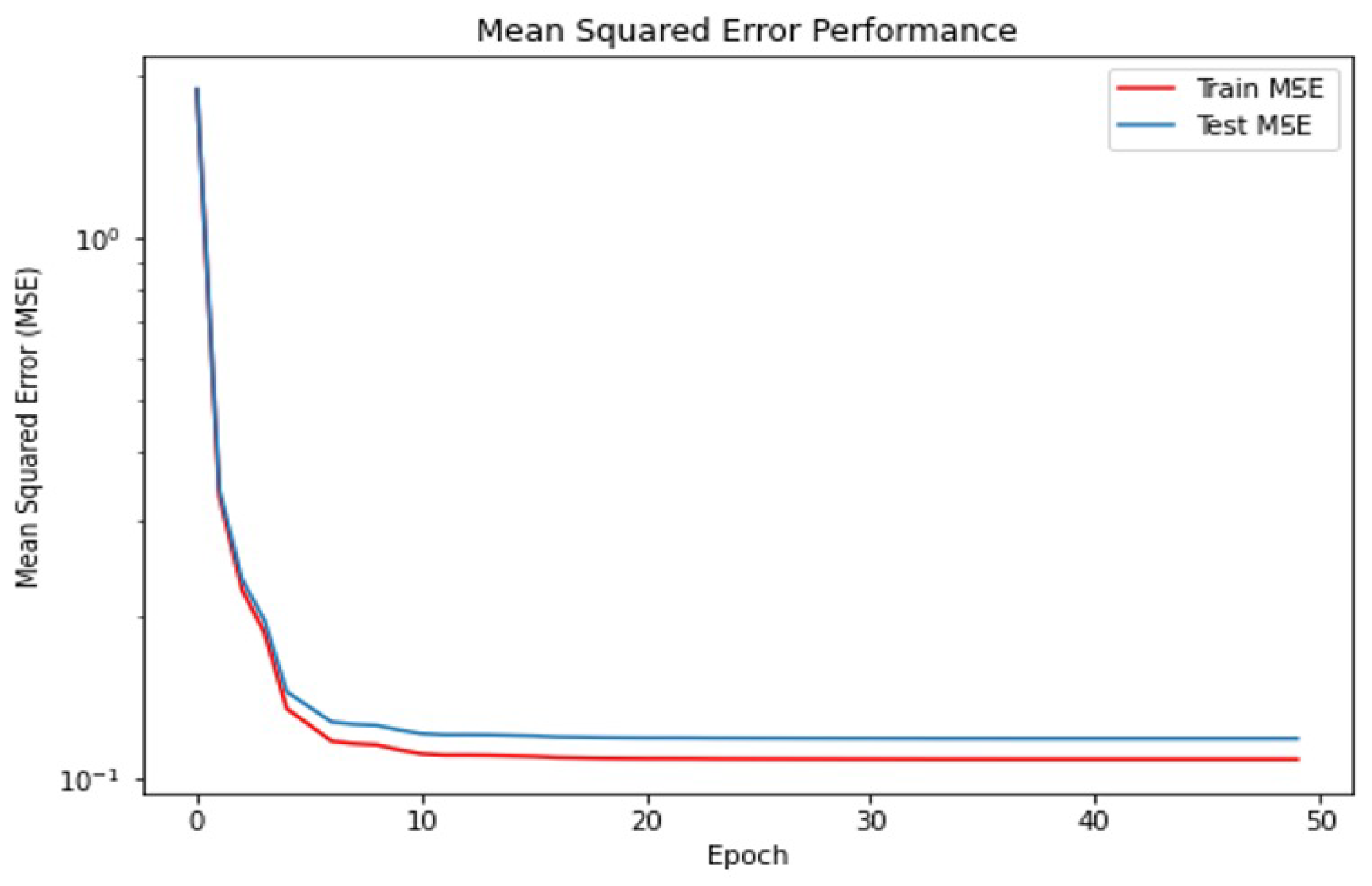
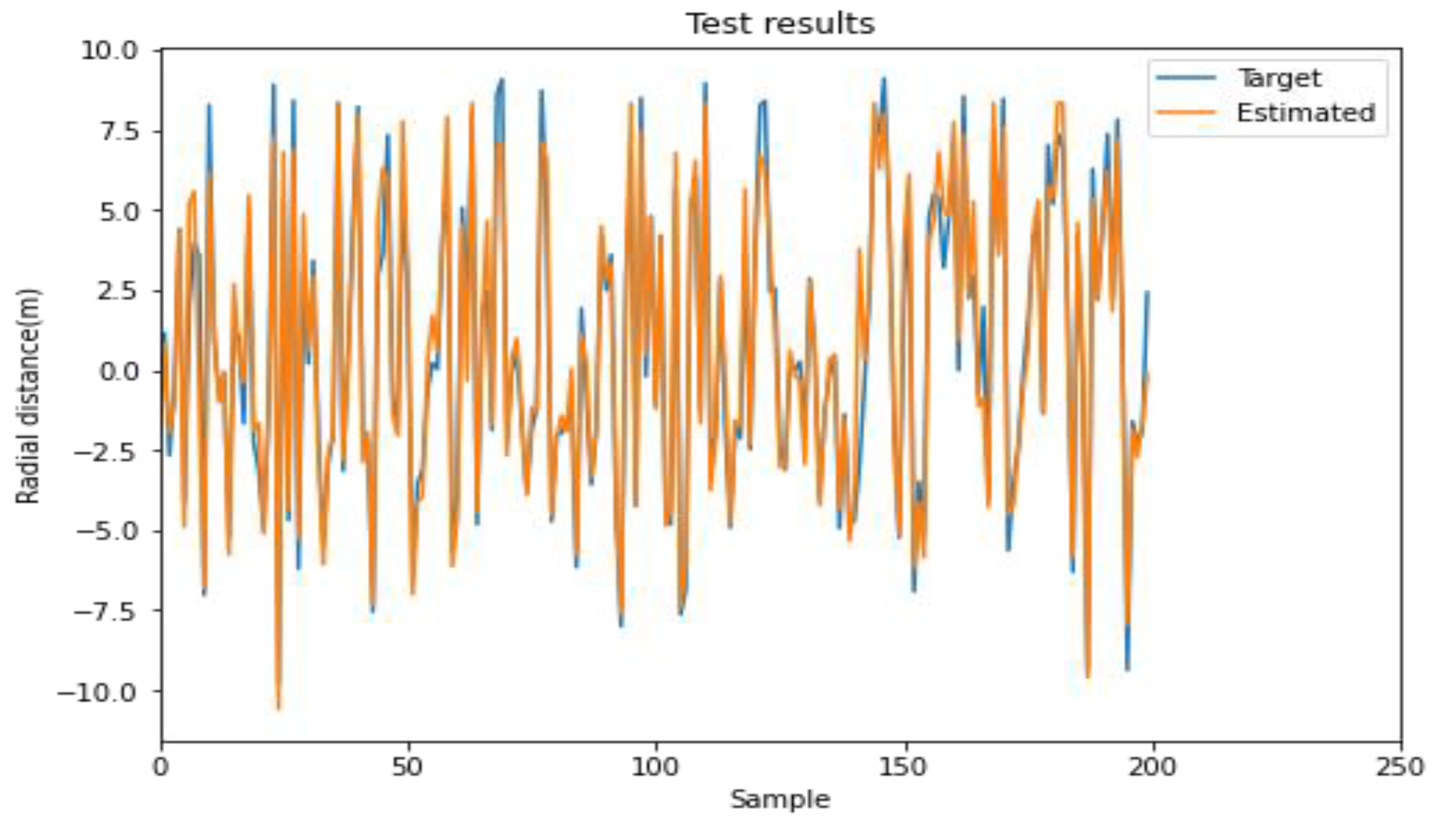
3. Results and Discussion

To complete the first stage of our proposed model, we employed the YOLOv7 algorithm for object detection, and conducted training using our prepared dataset. In order to ensure a fair comparison between YOLOv7 and Enhanced YOLOv7 + CBAM, we employed the same settings of the optimizer, learning rate, and input resolution for both algorithms to achieve optimum accuracy while reducing the required testing and training time.

As mentioned previously, data augmentation techniques including flipping, scaling, and adjustments to contrast, color, and brightness were utilized. The images were scaled to 640 × 640 pixels for testing and training in YOLOv7. The Adam optimizer, which has been shown to be effective for training deep learning models with high precision, was employed with a learning rate of 10⁻³ to prevent overfitting. A batch size of 16 and 4 workers were used to train the model and achieve the desired results. The training was carried out for 300 epochs and approximately 70,000 iterations; after every epoch, the validation dataset was used to evaluate the performance, and then the best model was saved. The validation dataset made up 20% of the entire samples. Finally, the test dataset was used to evaluate the performance of the best model.

To enhance the precision of the YOLO network, irrelevant classes that did not correspond to the objects present in the surroundings of autonomous vehicles (AVs) were removed. Our approach focuses on detecting three classes: cars, rear lights, and front lights. The training results of the YOLOv7 network were evaluated using our dataset, both with and without adding the attention module. The results are illustrated in Figure 5 and Figure 6.

As shown in these plots, in Figure 5, the average loss of the YOLOv7 network decreased to about 0.75 after about 70,000 iterations in the training process, and in Figure 6, decreased even further to about 0.69 after applying the attention mechanism. The achieved average loss takes into account the high variance in the size of detected classes (large vehicles compared to small car lights) and the high dynamics of the scenes.

We also evaluated the average loss in comparison to YOLOv3, a similar model used in [28]. YOLOv3 achieved an average training loss of 1.22, while our approach achieved higher accuracy in detecting objects of interest in AVs. This is demonstrated in Figure 7, which shows the implementation of the YOLOv7 algorithm in real-world images, indicating the effectiveness of our provided dataset in achieving the required results.

Evaluation Criteria

For the purpose of evaluating the YOLOv7 algorithm’s performance, the following evaluation indices were used: precision (P), mean average precision (mAP), recall (R), frames per second (FPS), and F1 score.

Precision is a valuable metric to consider when evaluating the accuracy of a model in predicting positive samples. It measures the proportion of true positive predictions made by the model out of all the samples predicted as positive. True positives represent correctly predicted positive samples. Higher precision scores indicate stronger positive sample prediction. The formula is as follows:

$$\mathrm{Precision}=\frac{\mathrm{TP}}{\mathrm{TP}+\mathrm{FP}}$$

(1)

Recall is a performance metric that measures the proportion of true positives identified by a model to the total of true positives and false negatives. It is useful for measuring the accuracy of a classification model when the dataset is unbalanced. Here is the calculation formula:

$$\mathrm{Recall}=\frac{\mathrm{TP}}{\mathrm{TP}+\mathrm{FN}}$$

(2)

To evaluate classification models, the F1 score is frequently used as a metric of accuracy. By combining precision and recall scores into a singular measurement, it offers an inclusive evaluation of the model’s performance. The calculation for F1 score involves determining the harmonic mean of precision and recall, which can be expressed using the formula provided:

$$\mathrm{F}1=\left(\frac{2}{{\mathrm{Recall}}^{-1}+{\mathrm{Precision}}^{-1}}\right)=2\frac{\mathrm{Precision}.\mathrm{Recall}}{\mathrm{Precision}+\mathrm{Recall}}$$

(3)

The mAP index is a measure of how accurately a model can detect objects in an image. It uses the COCO (Common Objects in Context) [58], standard to evaluate the performance of the model in terms of precision and recall. The mAP index is an effective metric for assessing the accuracy of object detection models; a higher mAP indicates more reliable detection and localization of objects.

The experiments described in this paper were performed on a computer system equipped with an NVIDIA Tesla T4 GPU (NVIDIA, Santa Clara, CA, USA) and 16 GB of RAM. The operating system used was Windows 10 (Microsoft, Redmond, WA, USA) and the deep learning framework used was PyTorch 1.7.0 (PyTorch, Warsaw, Poland).

After evaluating the two approaches under similar training settings, we achieved the results presented in

Table 1. Comparison of detection results between YOLOv7 and YOLOv7-CBAM.

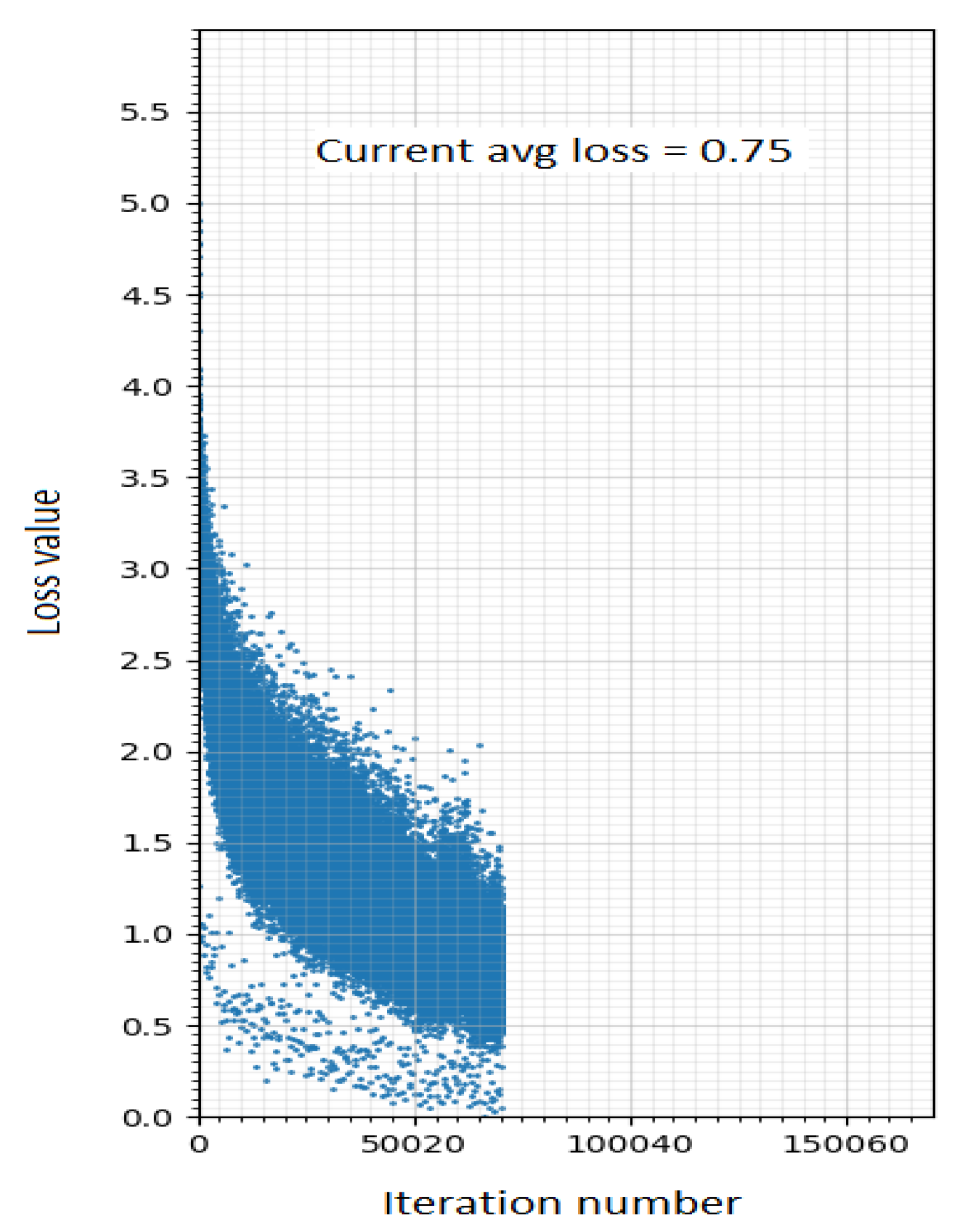
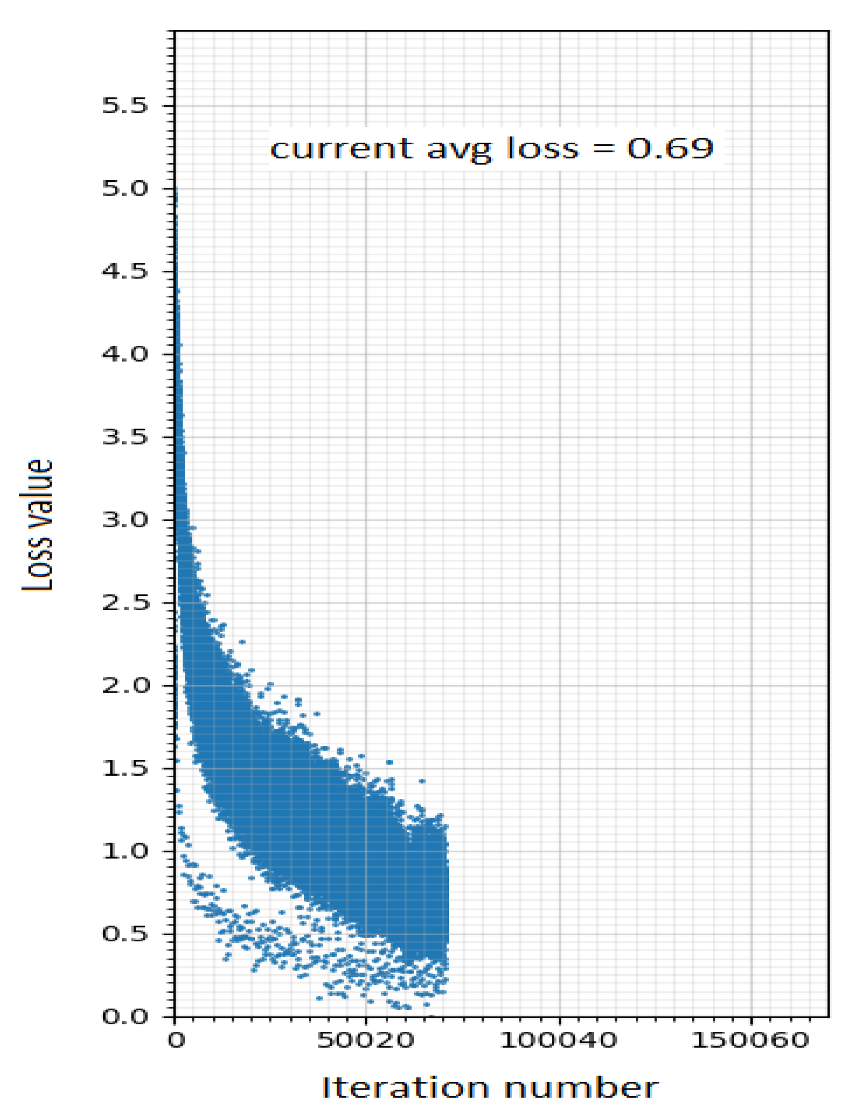
Method	Training Loss	Precision (P)	Recall (R)	[email protected]:0.95	[email protected]	F1	FPS
YOLOv7	0.75	0.7674	0.667	0.375	0.681	0.71	65
YOLOv7-CBAM	0.69	0.8056	0.6704	0.3824	0.7096	0.73	61

.

The analysis of results shows that the values in both models become closer to each other in the higher epochs, and that integrating the attention mechanism into the YOLOv7 architecture can result in improved accuracy in most of the metrics mentioned, while exhibiting a slightly lower speed. However, even slight improvements in detection accuracy in AVs are important.

In our study, we analyzed the computational efficiency of the two algorithms by comparing their FLOPs (floating point operations per second) parameter. Our findings suggest that the CBAM-YOLOv7 and original YOLOv7 algorithms have comparable levels of efficiency, with the CBAM-YOLOv7 model exhibiting a slightly higher FLOPS parameter value, which is increased by 0.6 G.

In Figure 8, we present a demonstration of the successful implementation of the YOLOv7-CBAM model in a Carla scene.

Figure 9 shows the test and train error histograms for the analysis of the precision of the multi-layer perceptron (MLP) network. According to these histograms, both test and train errors feature a zero-mean normal distribution, which means that significant errors had a negligible frequency. These results indicate that the MLP network has the ability to generate accurate predictions with a small number of outliers. This suggests that the MLP network has a good generalization ability and can be used for accurate prediction.

It is essential to consider that all three defined inputs for the MLP network may not be available simultaneously. For example, in real-world scenarios where a car’s lights are covered by other vehicles or not recognized by the YOLOv7 detection network, the first two inputs (x1 and x2) that rely on the car light information will be affected. However, the third input, which represents the height of the car’s bounding box, is resistant to such cases where a part of the car is unidentifiable [28].

To increase the robustness of the distance estimation model against such cases, we designed the MLP network to be resilient against missing inputs. Specifically, when information from two out of the three inputs is unavailable, the network ignores the first two inputs and processes only the third input. While this approach may result in lower accuracy in distance estimation [28], it allows the model to continue making distance estimates even when some inputs are unavailable, increasing the model’s robustness in challenging real-world scenarios.

In Figure 10, we observe the mean squared error (MSE) after fifty epochs. According to the plot, the train and test mean squared error converged to the value of 10⁻¹. This indicates the superb performance of the network in the estimation of the depth, both in new frames and the frames it learned.

Figure 11 presents a radial distance plot of the test data, demonstrating the network’s ability to accurately estimate the camera’s distance from the front vehicle. A total of 213 samples from a CARLA-captured frame constitute the test data. The blue line on the plot indicates the actual distance while the orange line indicates the estimated distance. The close proximity of the two lines demonstrates the network’s high accuracy in estimating the distance. The radial distance plot shows that the network’s estimates of the distance between the front vehicle and camera have a high correlation with the ground truth; the maximum training error is approximately 1.23 m, while the maximum testing error is about 1.48 m within a mid-range of under 50 m. This indicates that the network is capable of accurately estimating distances in the CARLA-captured frames.

To improve the performance and generalization of our distance estimation model in real-world scenarios, we trained and tested it using a comprehensive dataset of CARLA-captured frames from various weather simulations, including sunny, cloudy, and low-light nighttime conditions. This diverse dataset provided our model with the necessary reliability to estimate distances in a wide range of lighting and visibility scenarios, improving its ability to operate safely and effectively in the traffic scene. In Figure 12, we provide examples of the proposed model’s successful implementation in CARLA scenes with different light conditions. This figure displays bounding boxes and precision scores for car and rear and front light classes, and the distance is measured in meters.

The model’s ability to accurately detect objects and their spatial location in complex environments is due to its robustness in handling variations in scale, angle, and illumination. Furthermore, Figure 13 shows that the model was able to successfully detect objects in real-world traffic environments. These results show that the model is not only accurate in detection, but also resilient across a variety of conditions, making it a reliable and effective solution for AV distance estimation application.

We have shown that YOLOv7 has a better performance in comparison with the standard YOLOv3 with regard to detection accuracy. Due to the lack of a standard, direct comparisons are not straightforward in terms of the evaluation of distance estimation models. In order to compare the performance of our proposed model and evaluate it against other models, we consider similar distance estimation evaluation metrics to those defined in [61]. We utilized mean absolute error (MAE) as the error measurement in this study. With regard to the distance assessment quality, ε_R and ε_A metrics were defined in [61], which express the relative distance estimation and mean absolute errors. We can define the mean absolute distance error (MAE) as follows:

$${\epsilon }_A=\frac{1}{n}{\displaystyle \sum _{i=1}^n|d_i-{\stackrel{⌢}{d}}_i|,}$$

(4)

The mean relative distance error is definable as:

$${\epsilon }_R=\frac{1}{n}{\displaystyle \sum _{i=1}^n\frac{|d_i-{\stackrel{⌢}{d}}_i|}{\max (d_i,1)},}$$

(5)

where n stands for the number of bounding boxes found. In addition, d′ and d stand for the paired vectors of the predictions and ground truth, respectively.

Initially, we extracted car images from the dataset and then proceeded to employ the YOLOv7 algorithm to accurately detect the position of the cars and their respective lights. Then, we implemented the MLP network to estimate depth and determine the distance to the vehicle. Finally, we compared this predicted value to the labeled value in the KITTI dataset to evaluate the accuracy of our approach [62]. Figure 14 displays the histogram of the difference between the obtained distance and the distance specified in the dataset.

Then, we tested the capability of our approach in the accurate estimation of the distance to front vehicles, which was estimated by employing the defined ε_R and ε_A metrics. The metrics could only be estimated for detected boxes, and it was useless to assess the distance of undetected objects. In

Table 2. Comparison results of defined distance estimation.

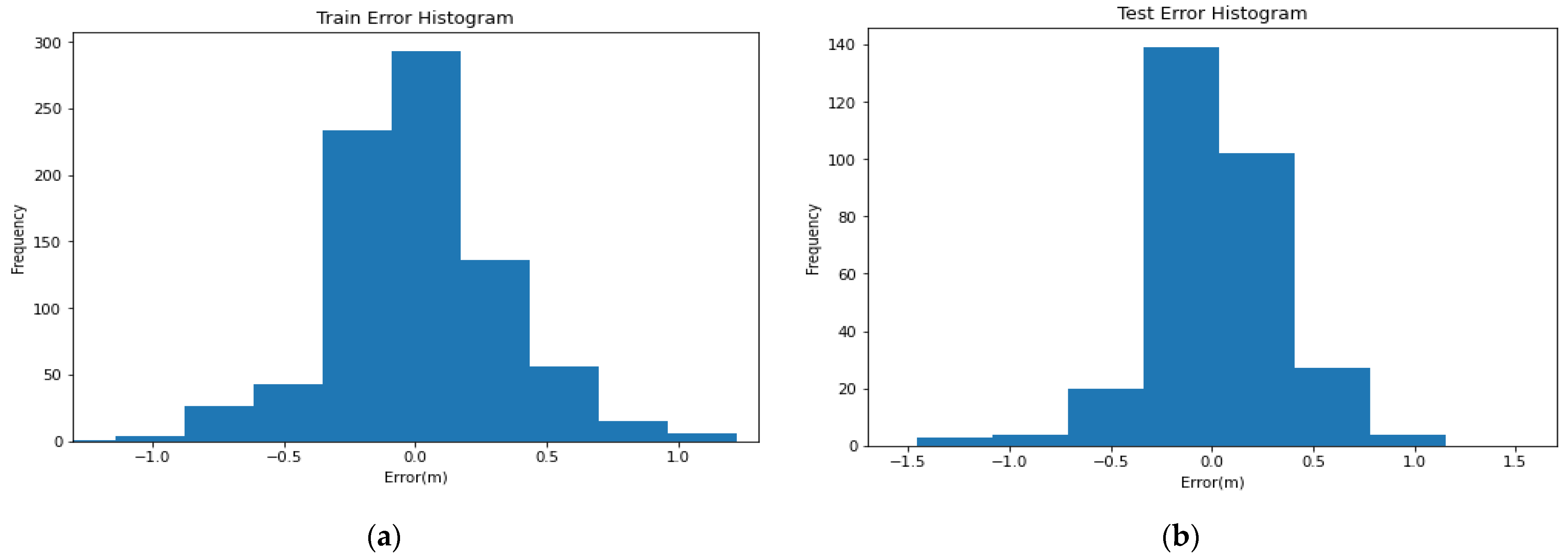
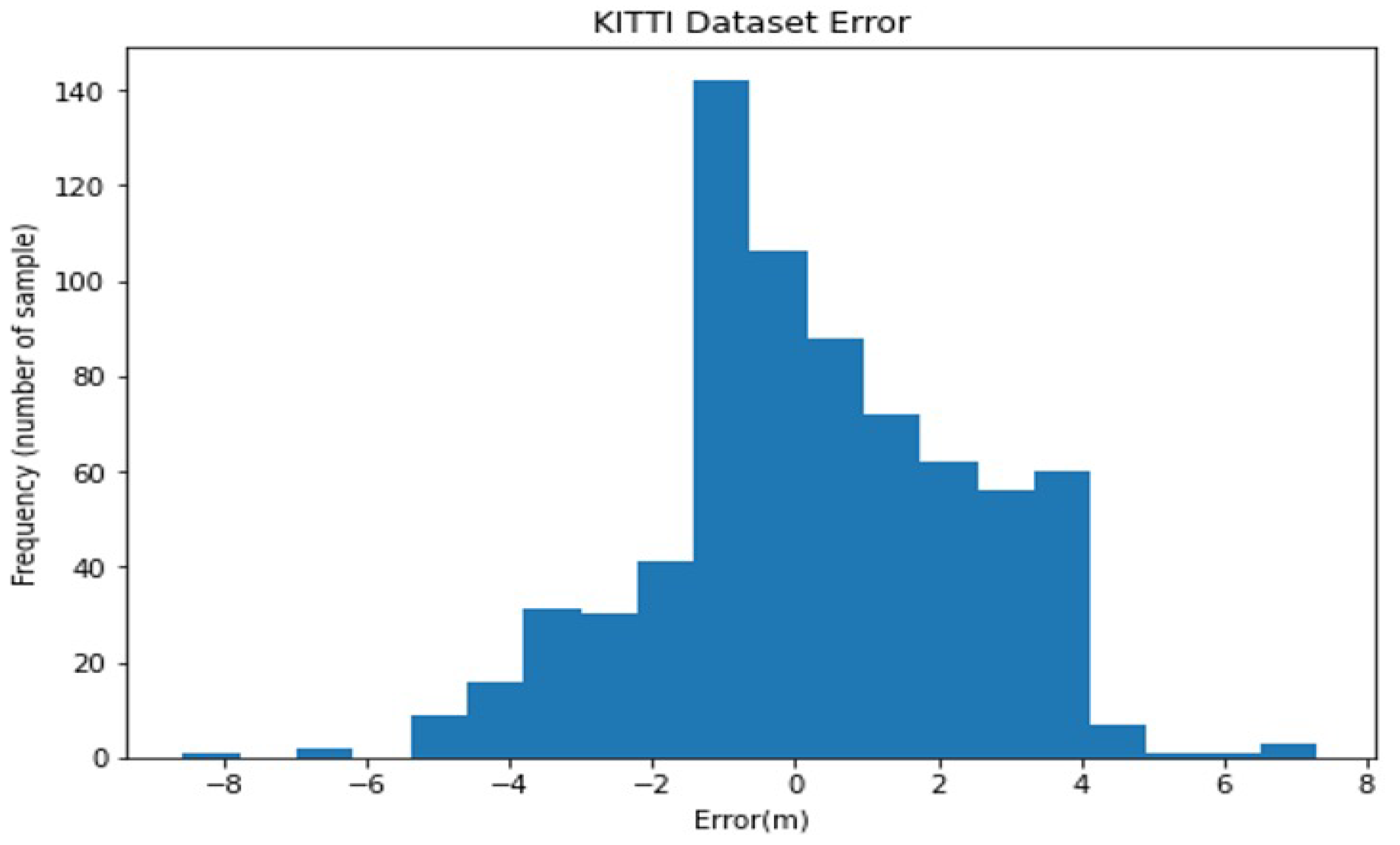
Method	Min	Mean	Max	εA	εR
Dist-YOLO [61]	−24.87	−0.81	14.47	2.49	0.11
Our method	−8.5	0.22	7.3	1.7	0.17

, the results include the mean distance error, as well as the maximum and minimum distance errors, expressed in meters, in the columns labeled Mean, Max, and Min, respectively, for comprehensiveness. Additionally, the value in column ε_R represents the relative distance error, where ε_R = 1 is equivalent to 100%.

As shown in Table 2, we achieved an MAE of 1.7 within mid-distances (<50 m). Another parameter used for comparison is the relative distance error, which reached 0.17. Given that authors report their results by employing a variety of settings, the numbers that follow are predominantly illustrative. On their KITTI validation dataset, Zhu et al. [63] obtained an ε_R value of 0.25. By only testing non-overlapping cars, Ali et al. [5] obtained an ε_R value of 0.29. In addition, by applying the same settings, they reported that DORN [64] yielded an ε_R value of 0.11. Mauri et al. [65] evaluated the performance of KITTI on three object classes, i.e., person, cyclist, and car. The results of their evaluation showed that the ε_R values achieved for these three classes in the test scenario were 0.42, 1.04, and 0.16, respectively. To compare the efficacy of our proposed method with existing approaches, we conducted experiments on the KITTI dataset. The results of our experiments show that that our proposed approach is a reasonable solution. Based on the fact that we are not sure about the uniformity of some of the parameters and settings they used, we may not be able to make a close comparison with the models mentioned in these articles.

The performance of our proposed model on real-world scenes from the KITTI dataset is displayed in Figure 15. The figure includes information about detected classes, predicted label values, and actual distance in meters.

4. Conclusions

Our proposed approach leverages the power of the YOLOv7 algorithm and a nonlinear model to enable accurate and fast detection and localization of cars and their lights in monocular images, even in challenging environments such as occluded traffic areas. The attention mechanism is utilized to highlight the most important features in the image for more accurate object detection, while the YOLOv7 network is enhanced with three CBAM modules to capture the spatial and channel-wise features of an image. Our comparative analysis revealed a remarkable improvement in precision, recall, F1, and mAP scores, indicating the better performance of our YOLOv7-CBAM method over the baseline YOLOv7 model. To provide a more direct comparison with existing studies, we evaluated our approach on the KITTI dataset, where we obtained a mean absolute distance error of 1.7 m and a mean relative distance error of 17%. These results clearly demonstrate the efficacy of our proposed method, which outperforms other approaches that rely solely on car height in the image. Moreover, our approach requires minimal computational overhead, making it suitable for a broad range of autonomous vehicle scenarios.

References

- Sreenivas, K.; Kamakshiprasad, V. Improved image tamper localisation using chaotic maps and self-recovery. J. Vis. Commun. Image Represent. 2017, 49, 164–176. [Google Scholar] [CrossRef]
- Singh, S. Critical Reasons for Crashes Investigated in the National Motor Vehicle Crash Causation Survey; National Highway Traffic Safety Administration: Washington, DC, USA, 2015.
- Mrovlje, J.; Vrancic, D. Distance measuring based on stereoscopic pictures. In Proceedings of the 9th International PhD Workshop on Systems and Control: Young Generation Viewpoint, Izola, Slovenia, 1–3 October 2008; pp. 1–6. [Google Scholar]
- Oberhammer, J.; Somjit, N.; Shah, U.; Baghchehsaraei, Z. RF MEMS for automotive radar. In Handbook of MEMS for Wireless and Mobile Applications; Elsevier: Amsterdam, The Netherlands, 2013; pp. 518–549. [Google Scholar]
- Ali, A.; Hassan, A.; Ali, A.R.; Khan, H.U.; Kazmi, W.; Zaheer, A. Real-time vehicle distance estimation using single view geometry. In Proceedings of the IEEE/CVF Winter Conference on Applications of Computer Vision, Snowmass, CO, USA, 1–5 March 2020; pp. 1111–1120. [Google Scholar]
- Khader, M.; Cherian, S. An Introduction to Automotive LIDAR; Texas Instruments: Dallas, TX, USA, 2020. [Google Scholar]
- Ding, M.; Zhang, Z.; Jiang, X.; Cao, Y. Vision-based distance measurement in advanced driving assistance systems. Appl. Sci. 2020, 10, 7276. [Google Scholar] [CrossRef]
- Raj, T.; Hanim Hashim, F.; Baseri Huddin, A.; Ibrahim, M.F.; Hussain, A. A survey on LiDAR scanning mechanisms. Electronics 2020, 9, 741. [Google Scholar] [CrossRef]
- Lim, Y.-C.; Lee, C.-H.; Kwon, S.; Jung, W.-Y. Distance estimation algorithm for both long and short ranges based on stereo vision system. In Proceedings of the 2008 IEEE Intelligent Vehicles Symposium, Eindhoven, The Netherlands, 4–6 June 2008; pp. 841–846. [Google Scholar]
- Liu, L.-C.; Fang, C.-Y.; Chen, S.-W. A novel distance estimation method leading a forward collision avoidance assist system for vehicles on highways. IEEE Trans. Intell. Transp. Syst. 2016, 18, 937–949. [Google Scholar] [CrossRef]
- Häne, C.; Sattler, T.; Pollefeys, M. Obstacle detection for self-driving cars using only monocular cameras and wheel odometry. In Proceedings of the 2015 IEEE/RSJ International Conference on Intelligent Robots and Systems (IROS), Hamburg, Germany, 28 September–2 October 2015; pp. 5101–5108. [Google Scholar]
- Zhang, K.; Xie, J.; Snavely, N.; Chen, Q. Depth sensing beyond LIDAR range. In Proceedings of the IEEE/CVF Conference on Computer Vision and Pattern Recognition, Seattle, WA, USA, 13–19 June 2020; pp. 1692–1700. [Google Scholar]
- Schastein, D.; Szeliski, R. A taxonomy and evaluation of dense two-frame stereo correspondence algorithm. Int. J. Comput. Vis. 2002, 47, 7–42. [Google Scholar] [CrossRef]
- Liang, H.; Ma, Z.; Zhang, Q. Self-supervised object distance estimation using a monocular camera. Sensors 2022, 22, 2936. [Google Scholar] [CrossRef]
- Tram, V.T.B.; Yoo, M. Vehicle-to-vehicle distance estimation using a low-resolution camera based on visible light communications. IEEE Access 2018, 6, 4521–4527. [Google Scholar] [CrossRef]
- Kim, G.; Cho, J.-S. Vision-based vehicle detection and inter-vehicle distance estimation. In Proceedings of the 2012 12th International Conference on Control, Automation and Systems, Jeju, Republic of Korea, 17–21 October 2012; pp. 625–629. [Google Scholar]
- Alhashim, I.; Wonka, P. High quality monocular depth estimation via transfer learning. arXiv 2018, arXiv:1812.11941. [Google Scholar]
- Hu, H.-N.; Cai, Q.-Z.; Wang, D.; Lin, J.; Sun, M.; Krahenbuhl, P.; Darrell, T.; Yu, F. Joint monocular 3D vehicle detection and tracking. In Proceedings of the IEEE/CVF International Conference on Computer Vision, Seoul, Republic of Korea, 27 October–2 November 2019; pp. 5390–5399. [Google Scholar]
- Weng, X.; Wang, J.; Held, D.; Kitani, K. 3d multi-object tracking: A baseline and new evaluation metrics. In Proceedings of the 2020 IEEE/RSJ International Conference on Intelligent Robots and Systems (IROS), Las Vegas, NV, USA, 24 October 2020–24 January 2021; pp. 10359–10366. [Google Scholar]
- Wei, X.; Xiao, C. MVAD: Monocular vision-based autonomous driving distance perception system. In Proceedings of the Third International Conference on Computer Vision and Data Mining (ICCVDM 2022), Hulun Buir, China, 19–21 August 2022; pp. 258–263. [Google Scholar]
- Tighkhorshid, A.; Tousi, S.M.A.; Nikoofard, A. Car depth estimation within a monocular image using a light CNN. J. Supercomput. 2023, 1–18. [Google Scholar] [CrossRef]
- Natanael, G.; Zet, C.; Foşalău, C. Estimating the distance to an object based on image processing. In Proceedings of the 2018 International Conference and Exposition on Electrical And Power Engineering (EPE), Iasi, Romania, 18–19 October 2018; pp. 211–216. [Google Scholar]
- Haseeb, M.A.; Ristić-Durrant, D.; Gräser, A. Long-range obstacle detection from a monocular camera. In Proceedings of the ACM Computer Science in Cars Symposium (CSCS), Munich, Germany, 13–14 September 2018; p. 3. [Google Scholar]
- Chen, Z.; Khemmar, R.; Decoux, B.; Atahouet, A.; Ertaud, J.-Y. Real time object detection, tracking, and distance and motion estimation based on deep learning: Application to smart mobility. In Proceedings of the 2019 Eighth International Conference on Emerging Security Technologies (EST), Colchester, UK, 22–24 July 2019; pp. 1–6. [Google Scholar]
- Godard, C.; Mac Aodha, O.; Brostow, G.J. Unsupervised monocular depth estimation with left-right consistency. In Proceedings of the IEEE Conference on Computer Vision and Pattern Recognition, Honolulu, HI, USA, 21–26 July 2017; pp. 270–279. [Google Scholar]
- Strbac, B.; Gostovic, M.; Lukac, Z.; Samardzija, D. YOLO multi-camera object detection and distance estimation. In Proceedings of the 2020 Zooming Innovation in Consumer Technologies Conference (ZINC), Novi Sad, Serbia, 26–27 May 2020; pp. 26–30. [Google Scholar]
- Zhe, T.; Huang, L.; Wu, Q.; Zhang, J.; Pei, C.; Li, L. Inter-vehicle distance estimation method based on monocular vision using 3D detection. IEEE Trans. Veh. Technol. 2020, 69, 4907–4919. [Google Scholar] [CrossRef]
- Tousi, S.M.A.; Khorramdel, J.; Lotfi, F.; Nikoofard, A.H.; Ardekani, A.N.; Taghirad, H.D. A New Approach To Estimate Depth of Cars Using a Monocular Image. In Proceedings of the 2020 8th Iranian Joint Congress on Fuzzy and Intelligent Systems (CFIS), Mashhad, Iran, 2–4 September 2020; pp. 045–050. [Google Scholar]
- Redmon, J.; Divvala, S.; Girshick, R.; Farhadi, A. You only look once: Unified, real-time object detection. In Proceedings of the IEEE Conference on Computer Vision and Pattern Recognition, Las Vegas, NV, USA, 27–30 June 2016; pp. 779–788. [Google Scholar]
- Wang, C.-Y.; Bochkovskiy, A.; Liao, H.-Y.M. YOLOv7: Trainable bag-of-freebies sets new state-of-the-art for real-time object detectors. arXiv 2022, arXiv:2207.02696. [Google Scholar]
- Müller, J.; Dietmayer, K. Detecting traffic lights by single shot detection. In Proceedings of the 2018 21st International Conference on Intelligent Transportation Systems (ITSC), Maui, HI, USA, 4–7 November 2018; pp. 266–273. [Google Scholar]
- Weber, M.; Wolf, P.; Zöllner, J.M. DeepTLR: A single deep convolutional network for detection and classification of traffic lights. In Proceedings of the 2016 IEEE Intelligent Vehicles Symposium (IV), Gothenburg, Sweden, 19–22 June 2016; pp. 342–348. [Google Scholar]
- Behrendt, K.; Novak, L.; Botros, R. A deep learning approach to traffic lights: Detection, tracking, and classification. In Proceedings of the 2017 IEEE International Conference on Robotics and Automation (ICRA), Singapore, 29 May–3 June 2017; pp. 1370–1377. [Google Scholar]
- Lee, H.S.; Kim, K. Simultaneous traffic sign detection and boundary estimation using convolutional neural network. IEEE Trans. Intell. Transp. Syst. 2018, 19, 1652–1663. [Google Scholar] [CrossRef]
- Luo, H.; Yang, Y.; Tong, B.; Wu, F.; Fan, B. Traffic sign recognition using a multi-task convolutional neural network. IEEE Trans. Intell. Transp. Syst. 2017, 19, 1100–1111. [Google Scholar] [CrossRef]
- Zhang, S.; Benenson, R.; Omran, M.; Hosang, J.; Schiele, B. Towards reaching human performance in pedestrian detection. IEEE Trans. Pattern Anal. Mach. Intell. 2017, 40, 973–986. [Google Scholar] [CrossRef]
- Zhang, L.; Lin, L.; Liang, X.; He, K. Is faster R-CNN doing well for pedestrian detection? In Proceedings of the Computer Vision–ECCV 2016: 14th European Conference, Amsterdam, The Netherlands, 11–14 October 2016; Part II 14. pp. 443–457. [Google Scholar]
- Li, B. 3d fully convolutional network for vehicle detection in point cloud. In Proceedings of the 2017 IEEE/RSJ International Conference on Intelligent Robots and Systems (IROS), Vancouver, BC, Canada, 24–28 September 2017; pp. 1513–1518. [Google Scholar]
- Li, B.; Zhang, T.; Xia, T. Vehicle detection from 3d lidar using fully convolutional network. arXiv 2016, arXiv:1608.07916. [Google Scholar]
- Fang, J.; Zhou, Y.; Yu, Y.; Du, S. Fine-grained vehicle model recognition using a coarse-to-fine convolutional neural network architecture. IEEE Trans. Intell. Transp. Syst. 2016, 18, 1782–1792. [Google Scholar] [CrossRef]
- Sermanet, P.; Eigen, D.; Zhang, X.; Mathieu, M.; Fergus, R.; LeCun, Y. Overfeat: Integrated recognition, localization and detection using convolutional networks. arXiv 2013, arXiv:1312.6229. [Google Scholar]
- Girshick, R.; Donahue, J.; Darrell, T.; Malik, J. Rich feature hierarchies for accurate object detection and semantic segmentation. In Proceedings of the IEEE Conference on Computer Vision and Pattern Recognition, Columbus, OH, USA, 23–28 June 2014; pp. 580–587. [Google Scholar]
- He, K.; Zhang, X.; Ren, S.; Sun, J. Spatial pyramid pooling in deep convolutional networks for visual recognition. IEEE Trans. Pattern Anal. Mach. Intell. 2015, 37, 1904–1916. [Google Scholar] [CrossRef]
- Girshick, R. Fast r-cnn. In Proceedings of the IEEE International Conference on Computer Vision, Santiago, Chile, 7–13 December 2015; pp. 1440–1448. [Google Scholar]
- Simonyan, K.; Zisserman, A. Very deep convolutional networks for large-scale image recognition. arXiv 2014, arXiv:1409.1556. [Google Scholar]
- He, K.; Zhang, X.; Ren, S.; Sun, J. Deep residual learning for image recognition. In Proceedings of the IEEE Conference on Computer Vision and Pattern Recognition, Las Vegas, NV, USA, 27–30 June 2016; pp. 770–778. [Google Scholar]
- Szegedy, C.; Liu, W.; Jia, Y.; Sermanet, P.; Reed, S.; Anguelov, D.; Erhan, D.; Vanhoucke, V.; Rabinovich, A. Going deeper with convolutions. In Proceedings of the IEEE Conference on Computer Vision and Pattern Recognition, Boston, MA, USA, 7–12 June 2015; pp. 1–9. [Google Scholar]
- Ren, S.; He, K.; Girshick, R.; Sun, J. Faster r-cnn: Towards real-time object detection with region proposal networks. Adv. Neural Inf. Process. Syst. 2015, 28. Available online: https://proceedings.neurips.cc/paper/2015/hash/14bfa6bb14875e45bba028a21ed38046-Abstract.html (accessed on 20 October 2022). [CrossRef]
- Bochkovskiy, A.; Wang, C.-Y.; Liao, H.-Y.M. Yolov4: Optimal speed and accuracy of object detection. arXiv 2020, arXiv:2004.10934. [Google Scholar]
- Zhu, X.; Lyu, S.; Wang, X.; Zhao, Q. TPH-YOLOv5: Improved YOLOv5 based on transformer prediction head for object detection on drone-captured scenarios. In Proceedings of the IEEE/CVF International Conference on Computer Vision, Montreal, BC, Canada, 11–17 October 2021; pp. 2778–2788. [Google Scholar]
- Wang, C.-Y.; Yeh, I.-H.; Liao, H.-Y.M. You only learn one representation: Unified network for multiple tasks. arXiv 2021, arXiv:2105.04206. [Google Scholar]
- Niu, Z.; Zhong, G.; Yu, H. A review on the attention mechanism of deep learning. Neurocomputing 2021, 452, 48–62. [Google Scholar] [CrossRef]
- Woo, S.; Park, J.; Lee, J.-Y.; Kweon, I.S. Cbam: Convolutional block attention module. In Proceedings of the European Conference on Computer Vision (ECCV), Munich, Germany, 8–14 September 2018; pp. 3–19. [Google Scholar]
- Muhammad, M.B.; Yeasin, M. Eigen-cam: Class activation map using principal components. In Proceedings of the 2020 International Joint Conference on Neural Networks (IJCNN), Glasgow, UK, 19–24 July 2020; pp. 1–7. [Google Scholar]
- Ying, X.; Wang, Y.; Wang, L.; Sheng, W.; An, W.; Guo, Y. A stereo attention module for stereo image super-resolution. IEEE Signal Process. Lett. 2020, 27, 496–500. [Google Scholar] [CrossRef]
- Jiang, K.; Xie, T.; Yan, R.; Wen, X.; Li, D.; Jiang, H.; Jiang, N.; Feng, L.; Duan, X.; Wang, J. An Attention Mechanism-Improved YOLOv7 Object Detection Algorithm for Hemp Duck Count Estimation. Agriculture 2022, 12, 1659. [Google Scholar] [CrossRef]
- Dosovitskiy, A.; Ros, G.; Codevilla, F.; Lopez, A.; Koltun, V. CARLA: An open urban driving simulator. In Proceedings of the Conference on Robot Learning, Mountain View, CA, USA, 13–15 November 2017; pp. 1–16. [Google Scholar]
- Lin, T.-Y.; Maire, M.; Belongie, S.; Hays, J.; Perona, P.; Ramanan, D.; Dollár, P.; Zitnick, C.L. Microsoft coco: Common objects in context. In Proceedings of the Computer Vision—ECCV 2014: 13th European Conference, Zurich, Switzerland, 6–12 September 2014; Part V 13. pp. 740–755. [Google Scholar]
- Domini, F.; Caudek, C. 3-D structure perceived from dynamic information: A new theory. Trends Cogn. Sci. 2003, 7, 444–449. [Google Scholar] [CrossRef]
- Reddy, N.D.; Vo, M.; Narasimhan, S.G. Carfusion: Combining point tracking and part detection for dynamic 3d reconstruction of vehicles. In Proceedings of the IEEE Conference on Computer Vision and Pattern Recognition, Salt Lake City, UT, USA, 18–23 June 2018; pp. 1906–1915. [Google Scholar]
- Vajgl, M.; Hurtik, P.; Nejezchleba, T. Dist-YOLO: Fast Object Detection with Distance Estimation. Appl. Sci. 2022, 12, 1354. [Google Scholar] [CrossRef]
- Geiger, A.; Lenz, P.; Urtasun, R. Are we ready for autonomous driving? The KITTI vision benchmark suite. In Proceedings of the 2012 IEEE Conference on Computer Vision and Pattern Recognition, Providence, RI, USA, 16–21 June 2012; pp. 3354–3361. [Google Scholar]
- Zhu, J.; Fang, Y. Learning object-specific distance from a monocular image. In Proceedings of the IEEE/CVF International Conference on Computer Vision, Seoul, Republic of Korea, 27 October–2 November 2019; pp. 3839–3848. [Google Scholar]
- Fu, H.; Gong, M.; Wang, C.; Batmanghelich, K.; Tao, D. Deep ordinal regression network for monocular depth estimation. In Proceedings of the IEEE Conference on Computer Vision and Pattern Recognition, Salt Lake City, UT, USA, 18–23 June 2018; pp. 2002–2011. [Google Scholar]
- Mauri, A.; Khemmar, R.; Decoux, B.; Haddad, M.; Boutteau, R. Real-time 3D multi-object detection and localization based on deep learning for road and railway smart mobility. J. Imaging 2021, 7, 145. [Google Scholar] [CrossRef]