Uncovering Equity and Travelers’ Behavior on the Expressway: A Case Study of Shandong, China

Abstract

Understanding equity and travelers’ behavior plays a key role in creating suitable strategies to promote the development of the expressway. Especially, finding clusters of expressway users could help managers provide targeted policies in order to enhance service quality. However, it is challenging to identify expressway travel behaviors, such as traffic flow distribution and users’ classification. Electronic toll collection (ETC) has been widely applied to improve expressway management, because it can record the origin–destination information of users. This paper proposes a framework to analyze the equity and travel behavior of expressway users with a large amount of ETC data. In the first stage, the Gini coefficient is adopted to analyze expressway equity. In the second stage, 12 kinds of indicators are extracted, including number of trips, car type, mean distance, etc. In the third stage, kmeans algorithm is adopted to cluster the users, based on the introduced indicators. Finally, we analyze the traffic flow distribution of each group by constructing a traffic flow network. The results show that the Gini coefficient is 0.4193, which demonstrates evident inequity in the expressway service. Moreover, statistical analysis shows that expressway flow is complicated and 70.77% of travelers do not make repeat trips. It is demonstrated that expressway users can be divided into six groups, and the flow networks of cluster 2 and cluster 3 are connected more closely and evenly than other clusters are.

1. Introduction

The expressway plays a significant role in transporting persons and goods in China, which greatly promotes regional development. During recent decades, expressways in China have gained remarkable growth and their total length reaches 0.161 million kilometers at the end of 2020. With the development of the expressway, traffic demand has grown rapidly. In daily operation, the expressway often suffers from congestion and unreliability due to the large volume of vehicles, bad weather and other stochastic factors [1,2,3]. On the other hand, there is high surplus capacity in off-peak hours. Operators have made great efforts to attract users to the expressway when there is surplus capacity. On the contrary, they control the number of users in peak hours. Dynamic pricing is an effective way to control the number of expressway users [4]. Therefore, grasping traffic flow distribution and users’ behavior is crucial for dynamic toll price strategies. However, it is difficult to obtain users’ patterns accurately because of the complex flow structure and their complex travel behavior.

It is imperative to understand travelers’ behaviors on the expressway, such as speeding behavior [5], lane choice behavior [6], route choice behavior [7], mode choice behavior [8], etc. Factors such as toll discount and travel time could impact transport mode choice. Lin et al. studied the mode choices of intercity travelers in Beijing during the 2017 Chinese Spring Festival holidays, and found that the expressway toll discount increased car use and decreased public transit usage [9]. Li et al. showed that travel distance, travel cost, travel time, safety, comfort and punctuality have significant impacts on intercity travel mode competition [10]. Recently, big data-related technologies have shed light on understanding travelers’ behaviors [11,12,13,14]. For example, express toll stations could provide a large number of records, including entrance and exit times, vehicle ID, etc.

OD demand is of significance for daily management and highway planning. OD demand is not only affected by socio-economic factors but also by stochastic factors, such as weather and free policy during holidays [15,16]. There are many models to estimate OD demand, such as the gravity model [17,18], Markov Chain [19], radiation model [20,21], Bayesian model [22], binomial model [23], etc. The gravity model is the most widely adopted in understanding traffic flow distributions and network properties, and is successfully applied in many transportation systems [24,25,26]. The gravity law indicates that the flow between two areas has positive correlations with node strengths and negative correlations with the distances between the two areas. Based on data mining and spatial analysis, the OD flow exhibits various cluster patterns in many fields [27,28,29]. There are two core categories of OD flow clusters [30]. One is focused on OD flow attributes, such as volume, distance, directions, etc. The other is focused on spatial distribution of OD flow in geographical space. The OD flow attributes can be achieved by complex network and machine learning methods [31,32,33,34], and spatial distributions can be yielded by a spatial statistics-based method and a density-based method [35,36].

Travelers are considered as customers of the expressway. Customer clustering is an important way for managers to analyze customer features and allocate service resources. In terms of traveler classification, there have been many studies involving various methods based on travel survey data [37,38,39]. With the development of modern detection devices, types of automatic collection data, such as mobile phone data and IC card data, have been used to analyze travelers’ behaviors [40,41]. For expressway users, these behaviors are complicated, affected by many factors such as travel purpose, travel distance and personal attributes.

Most previous studies of this customer segment utilized survey data to cluster travelers according to their characteristics. However, the achieved sample is small because surveys are time-consuming and expensive. Moreover, survey data find it hard to reflect dynamic travel characteristics. To fill this gap, we propose a data-driven framework to study user clusters based on extensive historic ETC data. ETC systems provide a large amount of data to track travelers’ movements, which enables studies of temporal and spatial characteristics. The equity of the expressway is one of the most important indicators reflecting the spatiotemporal characteristics of traffic flow. In this paper, we also intend to detect the traffic distribution equity of the expressway, which is measured by Gini coefficient and flow disequilibrium factor.

The rest of the paper is organized as follows. Section 2 reports on the methods. Section 3 gives the data description. Results are shown in Section 4. Section 5 provides the discussion. Section 6 concludes the paper.

2. Methods

In this paper, we first explore expressway equity and features of expressway users. Secondly, kmeans algorithm is proposed to cluster users. Thirdly, expressway demand networks based on different groups of users are constructed in order to analyze characteristics. Finally, we introduce network-based measures to evaluate the spatiotemporal characteristics of trip networks.

2.1. Expressway Equity

The Gini coefficient reflects the equity between traffic demand distribution and people who live in the studied areas. We aggregate the number of people by a Voronoi diagram created by the toll stations. Inequity means that some areas with a large number of people only account for a small number of expressway passengers. Moreover, we introduce the flow disequilibrium factor to reflect the flow equity between stations, along with direction.

(1)

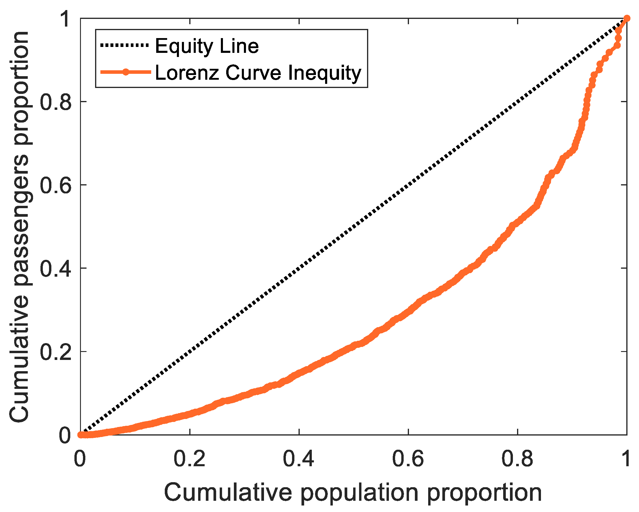
Lorenz curve and Gini coefficient

The Lorenz curve is a graphical representation of the cumulative distribution function of wealth across the population, which can be used not just for income but in other disciplines. The Gini coefficient is the ratio of area between the line of equality and Lorenz curve divided by the total area under the equality line [42]. In this paper, we adopt the Gini coefficient to reflect the equity of traveler distributions. The Gini coefficient can be approximated using the following equation.

$$G=1-{\displaystyle \sum _{k=1}^n(X_k-X_{k-1})(Y_k+Y_{k-1})}$$

(1)

where $X_k$ is the cumulative proportion of the population variable with $X_0=0$, $X_n=1$ and $Y_k$ is the cumulative proportion of the expressway service variable with $Y_0=0$ and $Y_n=1$.

(2)

Flow disequilibrium factor (FDF)

For the expressway flow network, there is difference between the two directions of a pair of nodes. In this paper, we adopt the flow disequilibrium factor to measure this, which is expressed as

$$FD{F}_{ij}=\frac{\max (w_{ij},w_{ji})}{w_{ij}+w_{ji}},w_{ij}+w_{ji}\ne 0$$

(2)

$$FDF=FD{F}_{ij}/t$$

(3)

where $w_{ij}$ and $w_{ji}$ are the number of travelers between node $i$ and $j$, and $t$ is the total number of OD pairs $w_{ij}+w_{ji}\ne 0$. Obviously, $FD{F}_{ij}$ and $FDF$ ranges from 0.5 to 1. A larger value means a more unbalanced flow.

2.2. Features of Expressway Users

In this part, we report on the features of users, including number of trips, car type, etc. These features could reflect characteristics of drivers’ mobility. Specifically, features are calculated for each user for all trips during the studied period. Based on these features, kmeans algorithm will be introduced to cluster the vehicles.

(1)

Number of trips (NT)

Number of trips for a user is defined as the total number of trips in the study period, which can reflect the travel frequency of the expressway users. In this paper, we divide NT values into five groups (0, 5): ‘NT 1’, (5, 10]: ‘NT 2’, (10, 20]: ‘NT 3’, (20, 50]: ‘NT 4’, (50, +∞): ‘NT 5’.

(2)

Unique number of trips (UNT)

Unique number of trips for a user is the number of trips without repeated origins and destinations. It can reflect the diversity of trips for expressway users. For example, commuters may have small UNT values. We divide UNT values into four groups. (0, 5): ‘UNT 1’, (5, 10]: ‘UNT 2’, (10, 15]: ‘UNT 3’, (15, +∞): ‘UNT 4’.

(3)

Car type (CT)

There are 16 kinds of vehicles on the expressway: ‘CT1’, ‘CT 2’, ‘CT 3’, ‘CT 4’, ‘CT 11’, ‘CT 12’, ‘CT 13’, ‘CT 14’, ‘CT 15’, ‘CT 16’, ‘CT 21’, ‘CT 22’, ‘CT 23’, ‘CT 24’, ‘CT 25’ and ‘CT 26’.

Table 1. Introduction of vehicle type.

Kinds of Car	Type	Explanation
Passenger cars	CT 1	The number of seats is smaller than 9
	CT 2	The number of seats is between 10 and 19
	CT 3	The number of seats is between 20 and 39
	CT 4	The number of seats is larger than 40
Trucks	CT 11	Two-axle with length smaller than 6 m and weight smaller than 4500 kg
	CT 12	Two-axle with length larger than 6 m and weight larger than CT11
	CT 13	Three-axle
	CT 14	Four-axle
	CT 15	Five-axle
	CT 16	Six-axle
Special motor vehicle	CT 21	-
	CT 22	-
	CT 23	-
	CT 24	-
	CT 25	-
	CT 26	-

shows the introduction of vehicle types. The travel characteristics of different types of vehicle are different. For example, trucks always travel more than private cars and pay more fees.

(4)

Mean distance (MD)

The mean value of travel distance is an important indicator to reflect users’ characteristics. In this paper, the MD is the mean value of all the trips of each user during the studied period. We divide MD values into four groups (0, 200): ‘MD 1’, (200, 500]: ‘MD 2’, (500, 1000]: ‘MD 3’, (1000, +∞): ‘MD 4’.

(5)

Total pay fee (TPF)

The total pay fee is related to the total travel distance, car type and discount fee. In this paper, TPF is the total value of pay fee of all the trips for each user. We divide TPF values into four groups. (0, 100): ‘TPF 1’, (100, 500]: ‘TPF 2’, (500, 1000]: ‘TPF 3’, (1000, +∞): ‘TPF 4’.

(6)

Total discount pay fee (TDPF)

There are many users who have a discount pay fee. Typically, the discount could promote the use of the expressway. In this paper, we use total discount pay fee as an import feature for users. TDPF is the total value of discount pay fee of all the trips for each user. We divide TDPF values into four groups (0, 5): ‘TDPF 1’, (5, 10]: ‘TDPF 2’, (10, 20]: ‘TDPF 3’, (20, +∞): ‘TDPF 4’.

(7)

Travel time (TT)

Travel time of all trips during the study periods is a crucial indicator, which is correlated with travel distance and travelers’ behaviors. TT is defined as the total value of travel time of all the trips for each user. We divide TT values into four groups (0, 100): ‘TT 1’, (100, 200]: ‘TT 2’, (200, 300]: ‘TT 3’, (300, +∞): ‘TT 4’.

(8)

Travel ratio (TR)

In this paper, we define travel ratio as the ratio between NT and UNT; a larger value means that there are more of the same trips in the study period. We divide TR values into four groups (0, 1): ‘TR 1’, (1, 2): ‘TR 2’, (2, 5): ‘TR 3’, (5, +∞): ‘TR 4’.

(9)

Maximum number of trips (MNT)

Maximum number of trips is defined as the maximum number of trips with same origin and destination. We divide MNT values into five groups (0, 5): ‘MNT 1’, (5, 10): ‘MNT 2’, (10, 15]: ‘MNT 3’, (15, 20]: ‘MNT 4’, (20, +∞): ‘MNT 5’.

(10)

Maximum distance of maximum trips (MDMT)

This is defined as the maximum distance among maximum trips with the same origin and destination. We divide MDMT values into four groups. [0, 200]: ‘MDMT 1’, (200, 500]: ‘MDMT 2’, (500, 1000]: ‘MDMT 3’, (1000, +∞): ‘MDMT 4’.

(11)

Enter hour of maximum trips (EMT)

The enter hour can reflect the time information for each trip. Commuters usually travel in the peak hours. We use actual hour for the indicator.

(12)

Number of maximum enter hour trips (NMET)

This is defined as the number of trips with maximum enter hour. We divide NMET values into five groups. [0, 1]: ‘NMET 1’, (1, 3]: ‘NMET 2’, (3, 5]: ‘NMET 3’, (5, 10]: ‘NMET 4’, (10, +∞): ‘NMET 5’.

2.3. Kmeans Clustering Algorithm

In this paper, we adopt a kmeans clustering algorithm to classify the groups of expressway users, which is an unsupervised learning method to gain the intrinsic features of data. Compared with other methods, it is easily implemented and with fast convergence, which is suitable for large scale data-set. There are many studies that use kmeans clustering algorithm to analyze the potential connections within data [43,44,45]. The classified groups are defined at the start. The algorithm contains four parts as follows [46,47].

(1) Choosing k data points as centroids.

(2) Calculating the distances between centroid points and other points, and classifying the closest point to the related group. There are several classic types of distances, such as Euclidean distance, Manhattan distance, cosine distance, and so on. In this paper, we use Euclidean distance, which is defined as follows:

$$d(x_i,x_j)=\sqrt{{\displaystyle \sum _{k=1}^m{\left(x_{ik}-x_{jk}\right)}^2}}$$

(4)

where $x_i$, $x_j$ are samples in m-dimensional space.

(3) After each point is classified into its group, all points are divided into k groups. Then the centroids of each group are recalculated.

(4) Repeat (2)–(3) until convergence. The convergence function is defined as follows:

$$J={\displaystyle \sum _{i=1}^k{\displaystyle {\sum }_{x\in C_i}d\left(x,u_i\right)}}$$

(5)

where $J$ is the minimum square error of $C=\left\{C_1,C_2,\cdots ,C_k\right\}$ achieved by the method. $u_i$ is the mean vector of the $C_i$, which is defined as

$$u_i=\frac{1}{\left|C_i\right|}{\displaystyle {\sum }_{x\in C_i}x}$$

(6)

Generally, the iteration stops due to two conditions: the center of cluster no longer changes, or the specified number of iterations has been reached.

In the kmeans algorithm, it is important to define the original number of divided groups k. In this paper, we use the silhouette coefficient to find suitable k. Silhouette coefficient is between −1 and 1, where values closer to 1 mean good performance [48].

2.4. Network-Based Measures

In this paper, we use a graph $G=(V,E,W)$ to represent the expressway trip network, where $V$ is the set of nodes, and $E$ is the set of edges. $G$ is a $N\times N$ adjacency matrix $e_{ij}$. $e_{ij}=1$, if there is an edge between node $i$ and node $j$; otherwise, $e_{ij}=0$. $N$ is the number of toll stations in the network. $W=\left\{w_{ij}|i,j=1,2,\cdots ,N,i\ne j\right\}$ is the set of weights and $w_{ij}$ can represent the weight of $e_{ij}$. In this paper, the weights are the number of trips.

(1)

Node degree

Node degree plays a key role in finding the important nodes in a complex network, which is defined as the number of nodes that interconnect. For the directed network, the degree is comprised of in-degree and out-degree. In-degree of a node $i$ means the number of nodes pointed to it, which is defined as

$$k_i^{in}={\displaystyle {\sum }_j{e}_{ji}}$$

(7)

Out-degree is the number of nodes pointing from the node $i$, which is expressed as

$$k_i^{out}={\displaystyle {\sum }_j{e}_{ij}}$$

(8)

The node degree is the sum of in-degree and out-degree as follows:

$$k_i=k_{in}+k_{out}$$

(9)

where $k_i$ is the node degree, and $e_{ij}$ and $e_{ji}$ are the connection status between node $i$ and node $j$.

(2)

Node strength

In this paper, node strength is defined as the traffic flow strength between nodes. Similar to node degree, it also contains in-strength and out-strength, which are defined as follows:

$$s_i^{in}={\displaystyle {\sum }_j{w}_{ji}}$$

(10)

$$s_i^{out}={\displaystyle {\sum }_j{w}_{ij}}$$

(11)

$$s_i=s_i^{in}+s_i^{out}$$

(12)

(3)

Betweenness

Betweenness is an index to measure the importance of a node for propagation information or flow, which is expressed as

$$C_B(v)={\displaystyle \sum _{s\ne t}\frac{{\sigma }_{st}(v)}{{\sigma }_{st}}}$$

(13)

where ${\sigma }_{st}$ is the number of shortest paths going from $s$ to $t$ and ${\sigma }_{st}(v)$ is the number of shortest paths going from $s$ to $t$ through the node $v$.

(4)

Clustering coefficient (CC)

Clustering coefficient is used to evaluate the connections among the neighbors of a node. It is defined as

$$C(v_i)=\frac{2e_i}{m_i(m_i-1)}$$

(14)

where $e_i$ is the number of edges among local neighbors of node $v_i$, and $m_i$ is the connection degree of neighbors of node $v_i$.

(5)

Degree correlation

In many complex networks, nodes have a tendency to connect with other nodes. Networks in which nodes with a high degree prefer to connect with other nodes with a high degree are called assortative networks. In contrast, networks in which nodes with a high degree tend to connect with nodes with a small degree are called disassortative networks. This can be expressed by

$$r=\frac{M^{-1}{\displaystyle {\sum }_i{j}_i{k}_i-{\left[M^{-1}{\displaystyle {\sum }_i\frac{1}{2}\left(j_i+k_i\right)}\right]}^2}}{M^{-1}{\displaystyle {\sum }_i\frac{1}{2}\left(j_i^2+k_i^2\right)-{\left[M^{-1}{\displaystyle {\sum }_i\frac{1}{2}\left(j_i+k_i\right)}\right]}^2}}$$

(15)

where $r$ is the correlation coefficient, and $j_i$ and $k_i$ are the degrees of the nodes at the ends of the $i$th links, with $i=1,\cdots ,M$. $r>0$ implies assortative network, $r<0$ indicates disassortative network, and $r=0$ an uncorrelated network.

(6)

Community structure

Community structure is ubiquitous in many kinds of complex networks. There are many edges in the community, but fewer edges between communities. In this paper, we use modularity to reflect the situation of a community, which is defined as

$$Q={\displaystyle \sum _i{e}_{ii}}-{\displaystyle \sum _{ijk}{e}_{ij}{e}_{ki}=Tre-‖e^2‖}$$

(16)

where $‖x‖$ indicates the sum of all elements of $x$. This can be achieved so that $0\le Q\le 1$. The larger the modularity, the stronger the community structure.

3. Data Description

The toll data used in this paper was collected from 1 March to 31 March 2021, in Shandong province, China, which is located along the eastern coast. Shandong province is one of the largest provinces in China with an area of 155,800 km² and a population of over 101 million. Shandong province is one of the top three provinces in terms of a high level of social and economic development in China at present. Total expressway length is more than 6300 km, playing an important role in the development of economy (see Figure 1).

There are 46.79 million items of toll data of 8,809,857 users, collected from all trips on the expressway that exited from stations in Shandong province. Specifically, the data contains all trips exiting from toll stations in Shandong province, no matter where the vehicles enter. Vehicles’ exits are recorded, including vehicles entering from stations outside Shandong province. The data contains the basic information for each vehicle, such as vehicle ID, entry station, entry time, exit station, exit time, car type, fee, discount fee, etc.

Table 2. Example of toll data.

Field	Example	Description
Vehicle ID	*** T3Y3	Vehicle plate number, unique
Entry station	Caoxian	Station name when a vehicle enters the expressway
Entry time	1 March 2021 10:09:39	Datetime when a vehicle enters the expressway
Exit station	Jinannan	Station name when a vehicle exits the expressway
Exit time	1 March 2021 14:01:40	Datetime when a vehicle exits the expressway
Car type	1	Kinds of vehicles
Fee	154	Fee paid for using the expressway
Discount fee	0	Discount fee for the trip
Other fields	…	…

*** stands for parts of vehicle ID in order to protect privacy of users.

shows an example of toll data. To protect privacy, we have hidden some information regarding vehicle plates.

4. Results

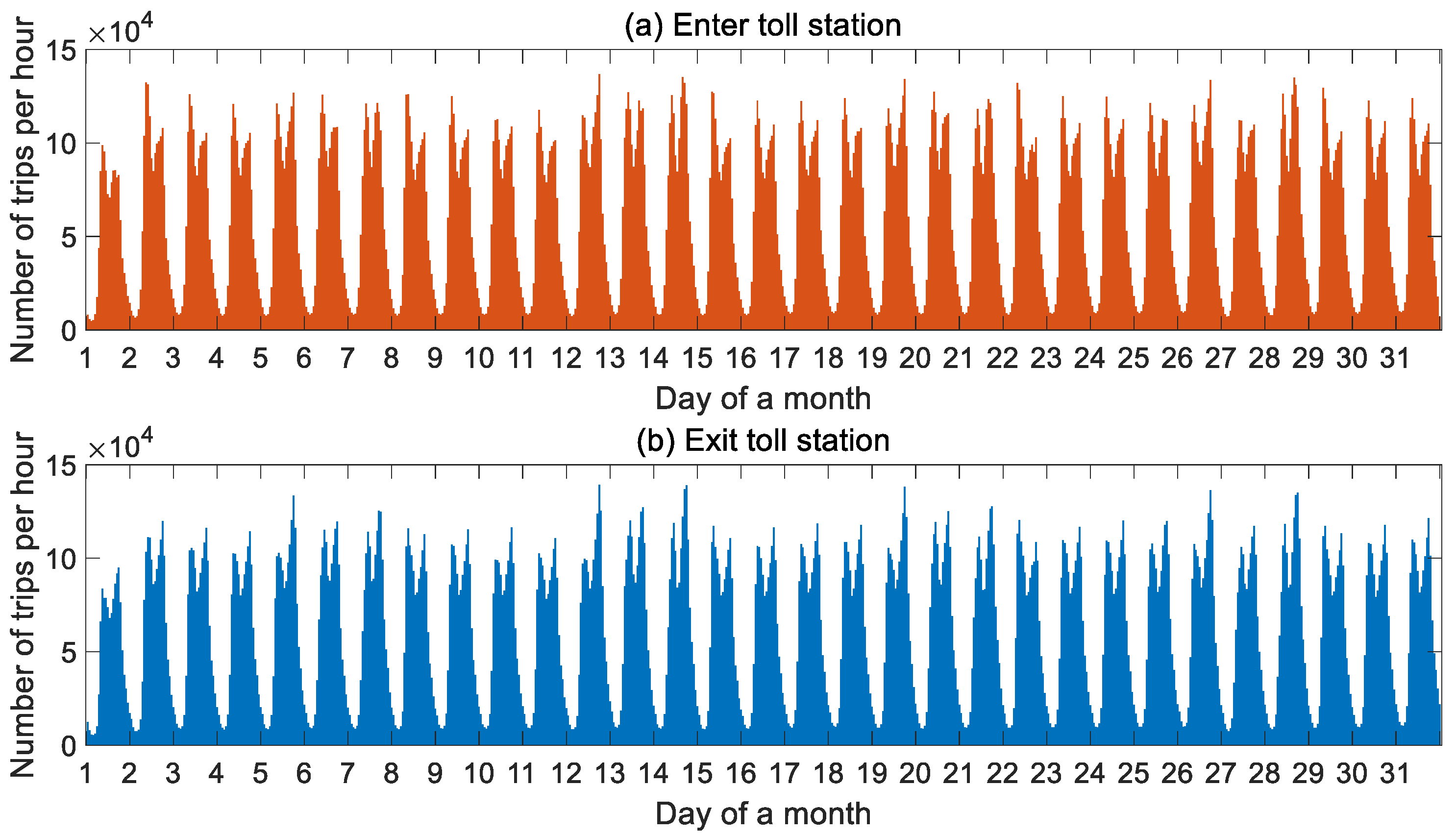
4.1. Temporal Characteristics of Expressway Users

In order to detect the temporal characteristics of expressway users, we plot the vehicle flow distributions in Figure 2. The number of entering toll stations and exiting toll station are collected for each hour. We can see that there are two peaks during the day: morning peak (7:00–10:00) and afternoon peak (14:00–17:00). For entering the toll station, the number of trips is larger in morning peak hours than afternoon peak hours. For exiting the toll station, the number of trips is smaller in morning peak hours than afternoon peak hours. There is no obvious difference between working days and weekends.

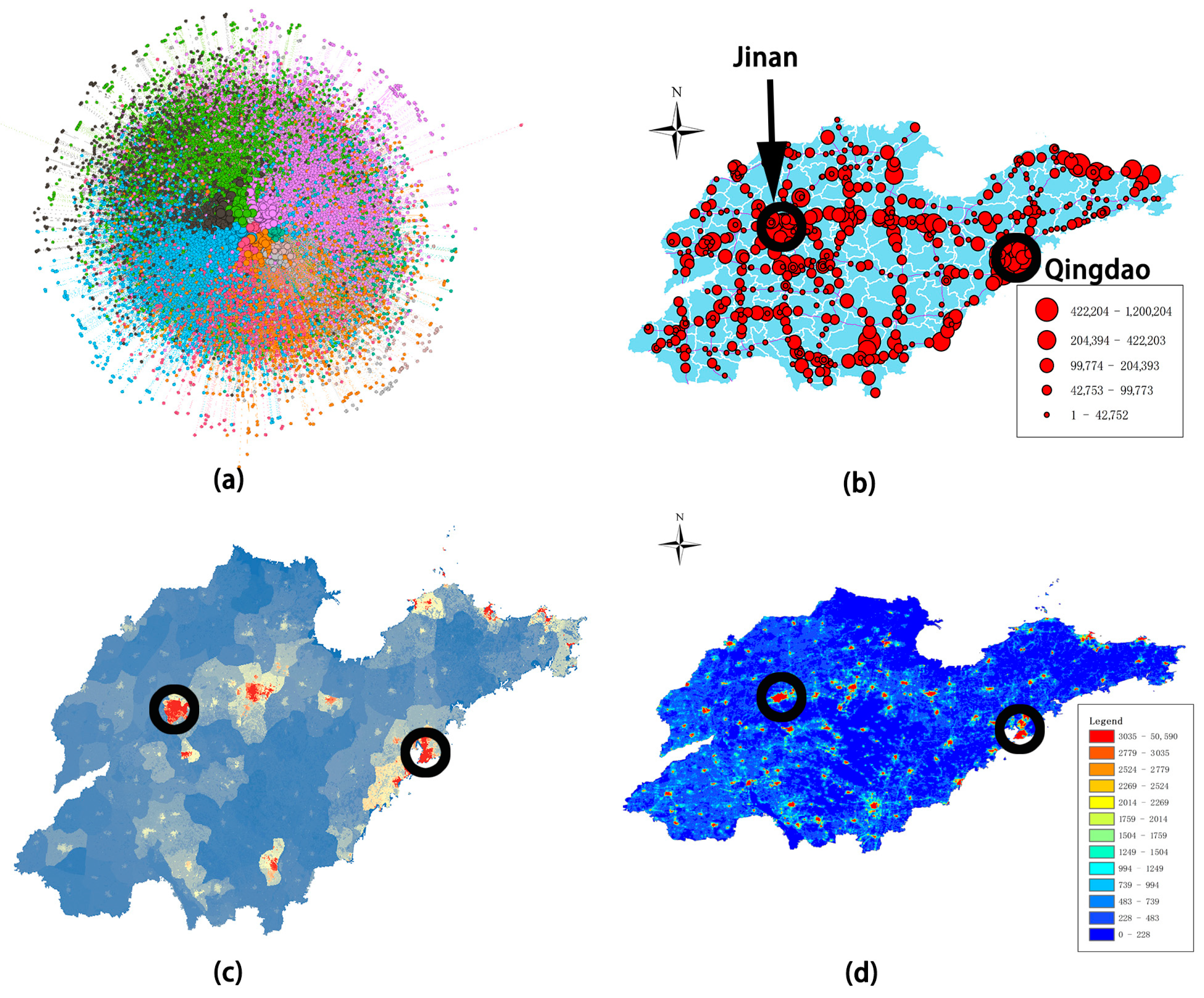
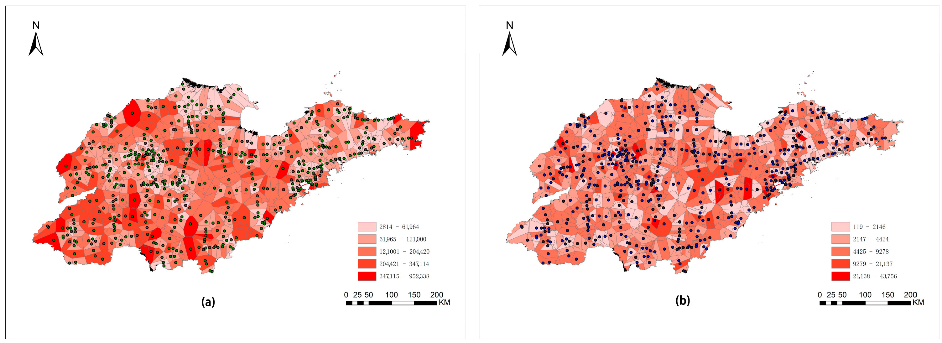
4.2. Spatial and Temporal Characteristics of Expressway Flow

Spatial distribution of traffic flow is of significance for understanding the structure of traffic demand. Figure 3a shows the complex network of expressway trips for all studied data, where node size represents the node degree and colors represents communities. Figure 3b illustrates the distributions of the number of vehicles for stations in Shandong, and larger nodes mean nodes with a larger value of node strength. Figure 3c,d exhibit the distributions of GDP and population of areas divided by 1 km × 1 km grids. We can see that the stations around Jinan and Qingdao have large values for exit vehicles, which is in line with the number of residents and economic development.

In order to understand the difference in network structures in different time periods, we divide a day into four time periods: 0:00–6:00, 6:00–12:00, 12:00–18:00 and 18:00–24:00. We choose a weekday (10 March, Wednesday) and a weekend day (13 March, Saturday) randomly, divide the weekday into four time periods: P1, P2, P3 and P4, and divide the weekend day into P5, P6, P7 and P8. Figure 4 illustrates the topological network structures in different time periods P1–P8, where node size represents the node degree and colors represent communities.

Table 3. Average value of indicators in different time periods.

	P1	P2	P3	P4	P5	P6	P7	P8
Degree	34.53	107.21	113.82	61.69	37.36	110.26	116.33	62.92
Strength	114.55	983.70	1130.42	384.36	127.93	1090.31	1280.12	436.33
CC	0.237	0.404	0.42	0.318	0.244	0.415	0.427	0.328
Betweenness	0.0024	0.0016	0.0015	0.0019	0.0024	0.0015	0.0015	0.0019
r	0.0159	0.0018	0.0050	0.0518	0.0316	0.0017	0.0097	0.0326
Modularity	0.522	0.591	0.609	0.598	0.518	0.602	0.617	0.62
FDF	0.8948	0.8348	0.8218	0.8557	0.8907	0.8269	0.8188	0.8501

gives the average value of indicators in different time periods. These indicators contain degree, strength, clustering coefficient (CC), betweenness, correlation coefficient (r) and modularity, which has been widely introduced in former studies [49]. It is noteworthy that the average degree and node strength of networks at weekends are larger than networks on weekdays, respectively. Additionally, the trip networks are connected sparely in P1 and closely in P3 from the point of view of node degree, which can be demonstrated by the average value of clustering coefficient. The networks of P1-P8 are assortative networks. The average values of FDF are larger than 0.8 in all eight networks, which implies that the traffic flows are seriously unbalanced in different directions.

4.3. Lorenz Curve of Expressway

A Voronoi diagram is a subdivision of an area by a set of points called generating points or generators. In the subdivision, each point is closer to one generating point than another generating point. In this part, we use toll stations of the expressway as generating points. Figure 5 shows the distributions of population and average number of entering and exiting vehicles per day, which is aggregated by Voronoi diagram.

Figure 6 shows the Lorenz curves of population and the average number of expressway vehicles per day. The Gini coefficient here measures the equity of distributions of people who use the expressway. It reflects equity of demand or need distribution. It can be understood simply that, if areas with a larger number of people have a larger number of expressway users, this shows equity; while some areas with a larger number of people have a smaller number of the expressway users, which shows inequity. The corresponding Gini coefficient is 0.4193, which indicates that there is evident inequity in the expressway service. We can see from the figure that 70.37% of people share 39.11% of the expressway service.

4.4. Characteristics of Traveler Behaviors

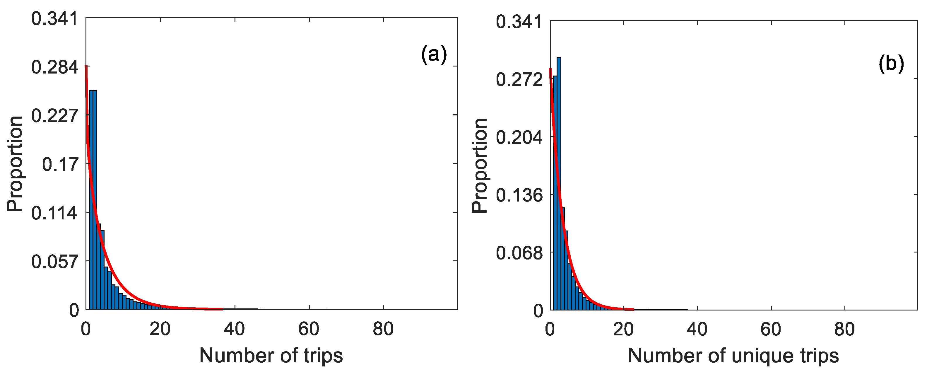
4.4.1. Number of Trips and Unique Trips

The number of trips for a user in a time period is an important indicator to measure the extent of using the expressway. Figure 7a,b plot the distributions of all users’ trips and unique trips, respectively. As can be seen, both indicators can be fitted by exponential distributions, which indicates that there is a small number of users using the expressway frequently. Only 20.29% of users travel more than five times during a month.

4.4.2. Basic Statistical Characteristics

Figure 8 shows the distribution of basic characteristics, including car type, mean distance, total pay fee, total discount pay fee, travel time and travel ratio. In this paper, there are 16 kinds of vehicle, which are numbered as ‘1’, ‘2’, ‘3’, ‘4’, ‘11’, ‘12’, ‘13’, ‘14’, ‘15’, ‘16’, ‘21’, ‘22’, ‘23’, ‘24’, ‘25’ and ‘26’. In more detail, ‘1’~‘4’ are four kinds of passenger vehicles, ‘11’~‘16’ represent six types of trucks, ‘21’~‘26’ are six kinds of repair vehicles. Figure 8a gives the distribution of different kinds of vehicle, which indicates that passenger vehicles with less than seven seats account for more than 80% of the total. Results imply that the distributions of mean distance, total pay fee, travel time and travel ratio can be fitted by exponential distributions. Total discount pay fee follows a lognormal distribution. The two kinds of distribution show that there is a small number of vehicles which have very large values for these indicators, and most vehicles have small values. Taking mean distance, for example, the mean distance of all trips for a vehicle is smaller than 200 km, accounting for 58.65%. Figure 8f shows the distributions of travel ratio between number of all trips and unique number. The results show that 70.77% of trips are without repeat trips.

4.4.3. Indicators for Maximum Repeating Trips

The maximum repeating trips related indicators are of significance for measuring the travel characteristics of vehicles. In this part, we plot the distributions of MNT, MDMT, EMT and NMET in Figure 9. We can see in Figure 9a that 93.36% of vehicles make repeating trips less than 5 times, which indicates a small number of commuters as expressway users. During these trips, 66.59% of distances are smaller than 200 km. Moreover, we plot the start hour of the most repeating trips for each vehicle, the results showing that 8:00–10:00 are the peak hours (Figure 9c). Figure 9d shows the number of maximum trips with the same entering hour, which indicates that 97.61% of vehicles start their trip at the same hour less than 5 times.

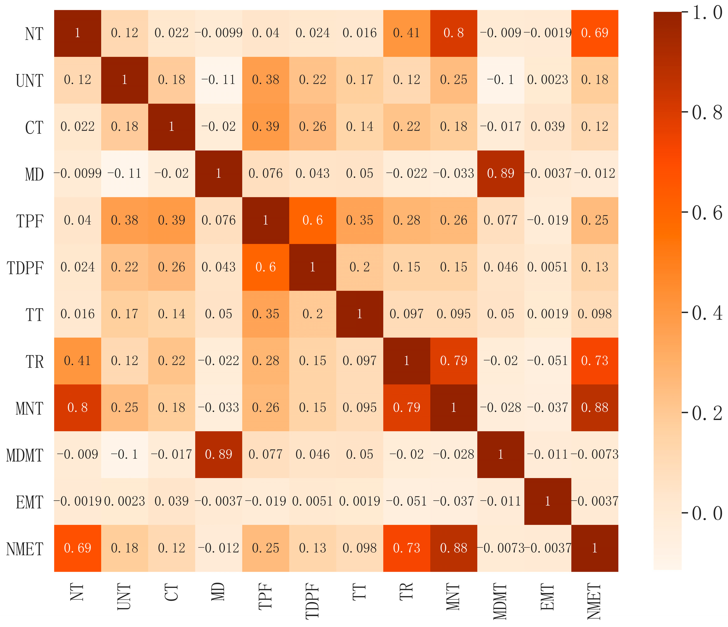
4.4.4. Correlations between Indicators

In this part, we use the Pearson coefficient to detect whether the chosen indicators have a linear relationship. If the relationship between any two indicators is strong and the Pearson coefficient is closer to 1, we will delete one indicator when clustering expressway users. Figure 10 shows the correlation between ten indicators by Pearson correlation coefficient. We can see that there is little positive relationship between MD and MDMT, which because there are many vehicles make only one trip during a month. Moreover, NMET is slightly positively related with MNT. However, it is found that the relationships between most indicators are not very strong, which means that the selected indicators can reflect the trips’ characteristics well.

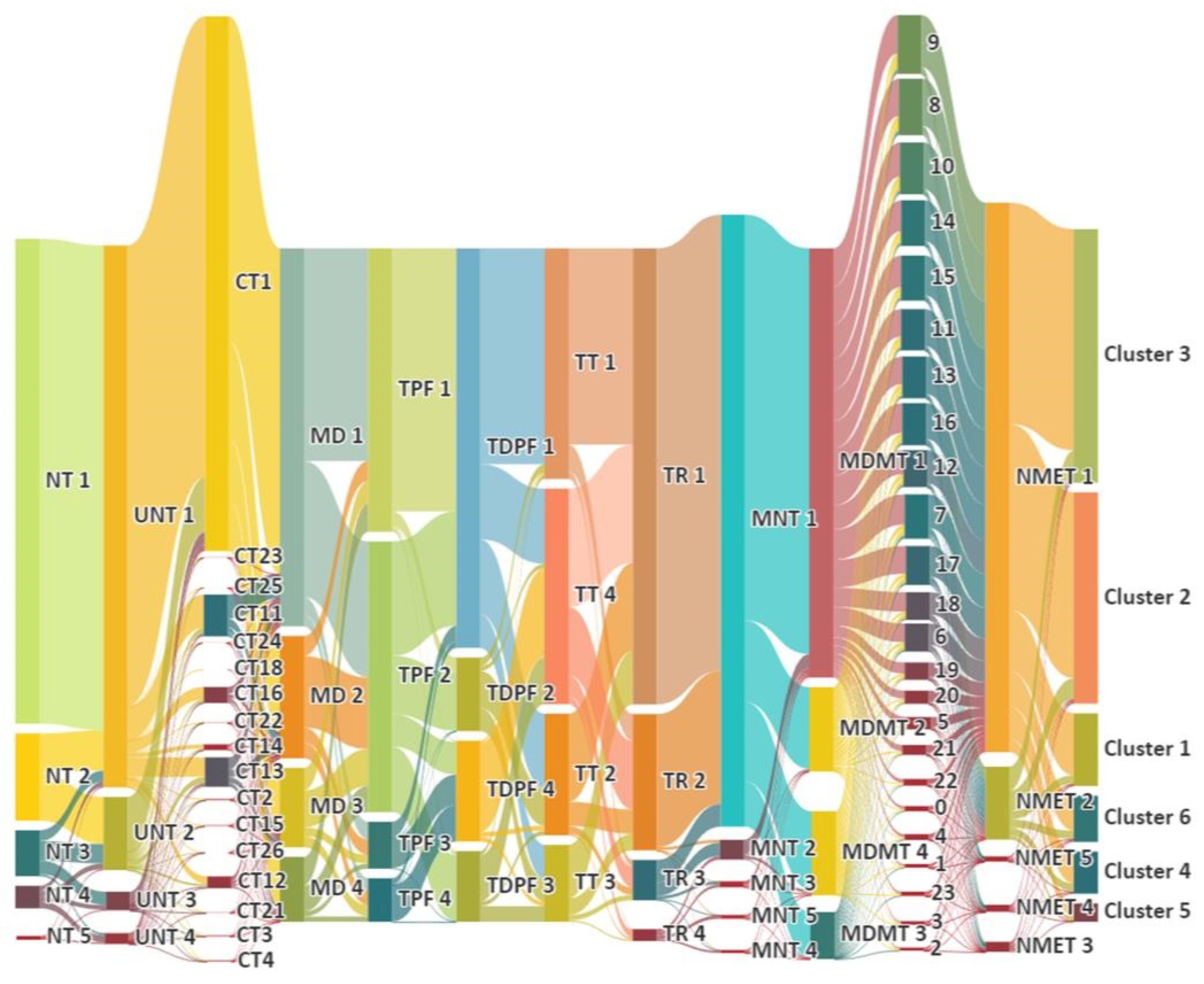
4.5. Clusters Based on Kmeans Algorithm

In this paper, we apply the kmeans algorithm to cluster vehicles using the proposed indicators, with 4, 5, 6, 7, 8, 9, 10 clusters.

Table 4. Average silhouette score with different clusters.

Clusters	4	5	6	7	8	9	10
Values	0.3852	0.4189	0.4383	0.4243	0.3624	0.3605	0.3521

illustrates the average silhouette score with different clusters. The largest value is 0.4383, which implies that six clusters is the best choice.

Figure 11 shows the distributions of indicators of different clusters, respectively. In total, the proportions of different clusters are 11.29%, 32.78%, 39.35%, 6.54%, 2.86% and 7.18%, respectively. We use cluster 1, cluster 2, cluster 3, cluster 4, cluster 5 and cluster 6 to represent these clusters. The characteristics of different clusters are as follows.

(1)

Cluster 1: As can be seen, this cluster mainly contains private vehicles. The average travel distance is very large. They prefer to travel after noon. Moreover, there are rare repeating trips.

(2)

Cluster 2: This cluster mainly contain private vehicles. The average travel distance of most vehicles is short. There is less discount pay fee and they prefer to travel after noon.

(3)

Cluster 3: The components of this cluster are similar to those of cluster 2. The average travel distance is larger than that of cluster 2. They prefer to travel before noon.

(4)

Cluster 4: This cluster consists of private vehicles and several kinds of vehicle that transport people. They prefer to travel between 14:00–22:00.

(5)

Cluster 5: This group contains most car types making long distance trips. The range of trip start time is wide.

(6)

Cluster 6: This group is similar to cluster 5, which contains most car types. The travel distance is shorter than that of cluster 5. They prefer to travel between 5:00–12:00.

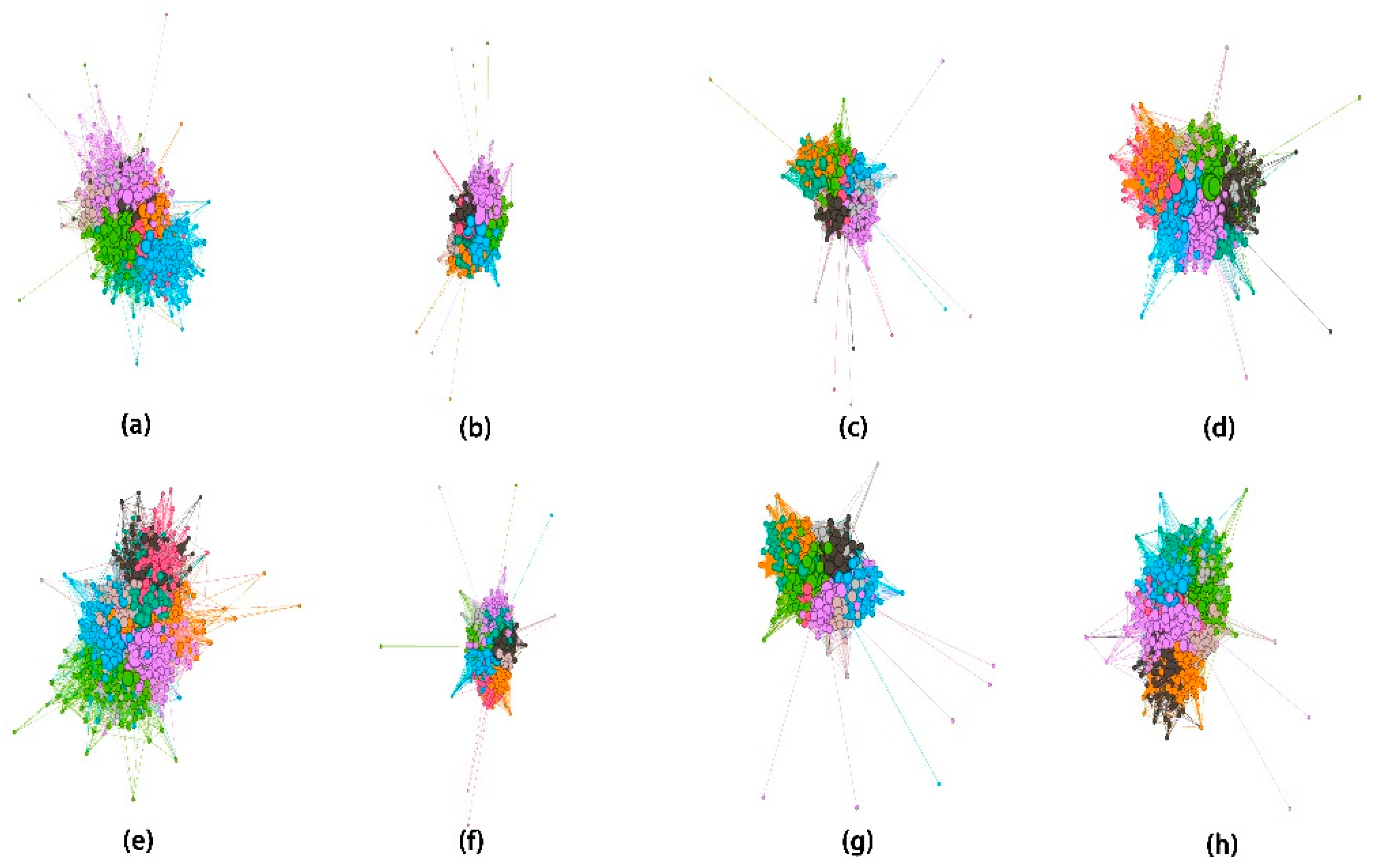
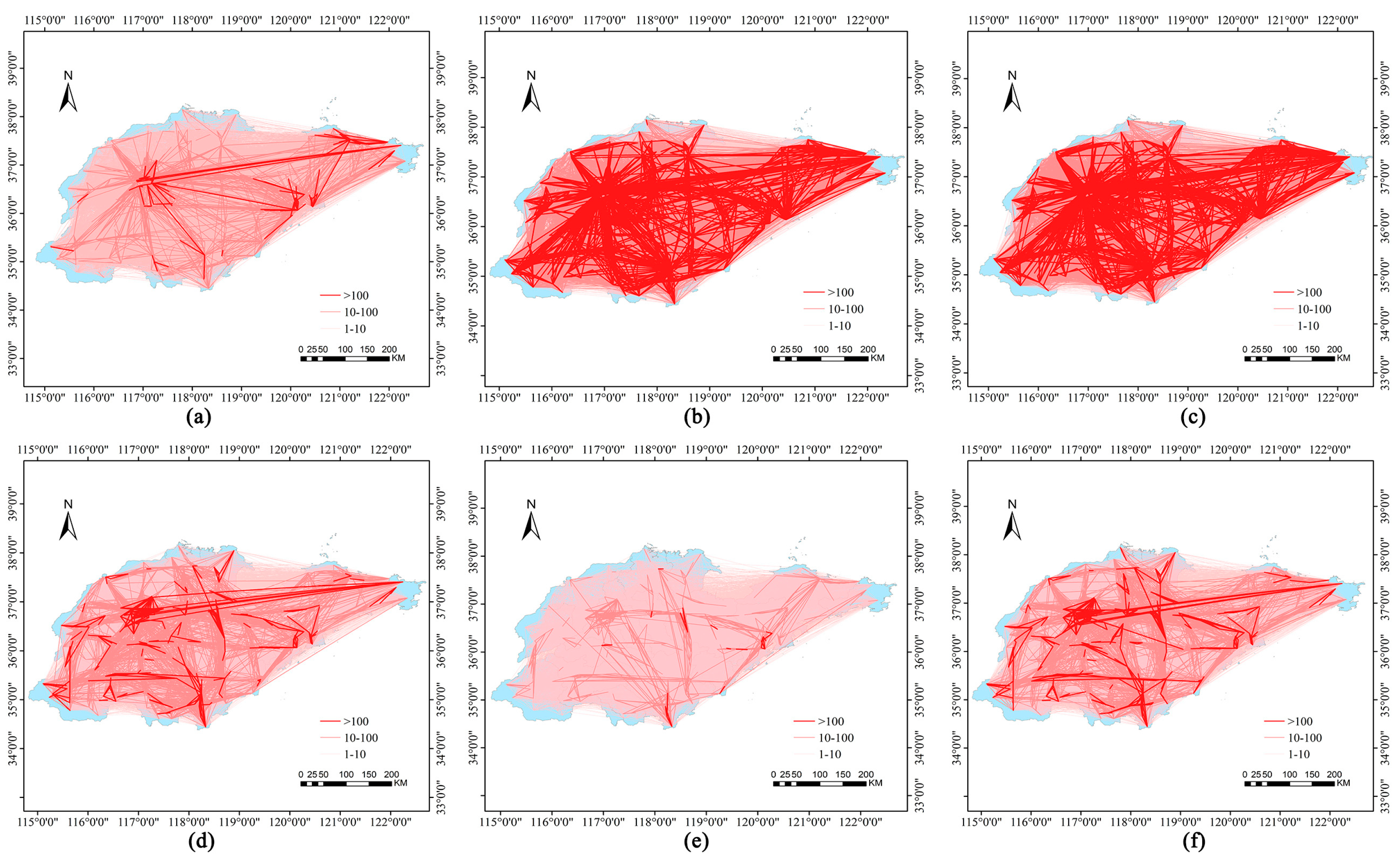
4.6. Expressway Flow Characteristics of Different Clusters

In order to understand the characteristics of the expressway flow of different clusters, Figure 12 exhibits the flow distributions for six clusters. Overall, the results imply that there is a small proportion of the expressway flow with a large value for all clusters. The number of trips with 100 or more vehicles account for 1.73%, 3.69%, 3.68, 0.89%, 0.49% and 1.1% for cluster 1, cluster 2, cluster 3, cluster 4, cluster 5 and cluster 6, respectively.

Table 5. Average value of indicators for different user clusters.

	Cluster 1	Cluster 2	Cluster 3	Cluster 4	Cluster 5	Cluster 6
N	516	538	545	521	515	520
Degree	50.73	105.19	230.96	64.84	32.52	65.31
Strength	713.79	2443.64	5632.87	465.71	158.53	529.03
CC	0.220	0.292	0.606	0.211	0.162	0.214
Betweenness	0.0014	0.0010	0.0009	0.0013	0.0016	0.0013
r	−0.1609	−0.0044	−0.0580	0.0111	−0.0416	0.0235
Modularity	0.593	0.591	0.577	0.554	0.527	0.578
FDF	0.8437	0.7752	0.7712	0.8326	0.8720	0.8296

shows the average value of indicators for different user clusters. It is found that network connectivity is positively correlated with the size of clusters. The network structures of six clusters are similar, where the cluster coefficient is large and betweenness is small. There is no evident tendency towards connections for nodes in the network. The FDF is large, which means that the flows between stations are unbalanced in terms of direction. The strength of cluster 2 and cluster 3 is larger than that of other clusters, which indicates that passenger cars have more flow strength between origin-destinations than other vehicles.

5. Discussion

The expressway plays a key role in transporting people and goods in China. Understanding its spatiotemporal characteristics and user classifications could help managers provide better services. User classification is important for making targeted policies to improve service quality, for example, giving a discount to people at night who frequently use the expressway, in order to reduce traffic congestion. Previous studies did much work with survey data, which could collect specific information such as personal attributes, travel characteristics and travelers’ satisfaction [50]. However, survey data cannot reflect the dynamic and long-term characteristics of the expressway user. ETC data could record much information, such as entry time, entry station, exit time, exit station, travel distance, fare, etc., which provides valuable resources to analyze expressway networks or travelers’ characteristics. Previous studies prefer to use Recency (R), Frequency (F) and Monetary (M) to create customer segments [51,52,53]. These three indicators cannot reflect some features of travelers, such as travel distance, vehicle type, repeating trips, etc. In this paper, we use12 kinds of features of travelers, which contains both traditional features and features not considered in previous studies. For example, we consider some features of travelers’ maximum trips, such as entry hour. Based on these indicators, our study could make more suitable classifications. Our study suggests that expressway users can be divided into six groups.

Spatiotemporal characteristics, such as equity of travel flow, can help mangers locate the weak point for services. Chen et al. found that passenger-car flow rate distribution for the expressway shows a dual-core, polycentric dispersed structure that is weakly concentric [54]. In the past two decades, many kinds of transport networks, such as transit, air transport and railways, have been widely analyzed, but the expressway trip network has seldom been explored. In this paper, we analyze the flow characteristics of the expressway network by mining a large amount of ETC data. Especially, we analyze the traffic flow distribution equity of the expressway by Gini coefficient and flow disequilibrium factor. We found that the Gini coefficient is 0.4193, which indicates an evident inequity in the expressway service. Managers should pay attention to those areas with numerous inhabitants and fewer expressway users when building new expressways.

The limitations of this study are as follows. Long-term data are better for traveler classification. In this paper, we only use one-month data due to data availability. Other travel modes, such as train and airplane, may impact the expressway flow distribution. This paper did not consider these impact factors.

Future study will focus on making exclusive policies for different kinds of traveler to enhance benefits and reduce congestion. Moreover, we intend to use multisource data to make the traveler segment more accurate. In addition, short-term traffic flow for the expressway network will be studied.

6. Conclusions

The expressway is an import transportation system, which plays a backbone role for intercity transport of people and goods. How to improve service quality and enhance profit becomes a crucial problem for operators, because it is faced with competition from other transportation systems. Understanding the characteristics and classification of expressway users is significant for policymaking, such as dynamic pricing. The ETC data could record users’ information for travel time, travel distance, pay fee, etc., which is a valuable source in studying the classification of expressway users.

This paper proposes a framework to analyze the equity and travel behavior of expressway users, with a large amount of ETC data. In the first stage, this paper adopted the Gini coefficient to measure the equity of the expressway. Then, 12 kinds of indicators deriving from the original ETC data are proposed, including number of trips, car type, mean distance, etc. Furthermore, this paper proposed a framework to classify expressway users by kmeans algorithm. Finally, we construct trip networks according to clusters. The results show that the Gini coefficient is 0.4193, which indicates that there is evident inequity in the expressway service. Statistical results show that expressway flow is complex and there is only a small proportion of users who make repeating trips during a month. From this perspective, operators should try their best to attract users. It is found that six clusters is the best form of classification. We analyze the differences between groups in the suggested indicators. It is seen that the flow networks of cluster 2 and cluster 3 are connected more closely and evenly than other clusters.

This paper can provide some suggestions for dynamic price policy and service quality improvement. Future study will focus on dynamic price policymaking and spatiotemporal characteristics of expressway flow prediction.

References

1. Fei, W.P.G.; Song, H.; Zang, J.R.; Gao, Y.; Sun, J.P.; Yu, L. Framework Model for Time-variant Propagation Speed and Congestion Boundary by Incident on Expressways. IET Intell. Transp. Syst. 2017, 11, 10–17. [Google Scholar] [CrossRef]
2. Zhang, C.; Qin, J.H.; Zhang, M.; Zhang, H.; Hou, Y.D. Practical Road-resistance Functions for Expressway Work Zones in Occupied Lane Conditions. Sustainability 2019, 11, 382. [Google Scholar] [CrossRef]
3. Zou, Y.J.; Zhu, T.; Xie, Y.F.; Li, L.B.; Chen, Y. Examining the Impact of Adverse Weather on Travel Time Reliability of Urban Corridors in Shanghai. J. Adv. Transp. 2020, 2020, 8860277. [Google Scholar] [CrossRef]
4. Shukla, A.; Bhattacharya, P.; Tanwar, S.; Kumar, N.; Guizani, M. DwaRa: A Deep Learning-based Dynamic Toll Pricing Scheme for Intelligent Transportation Systems. IEEE Trans. Veh. Technol. 2020, 69, 12510–12520. [Google Scholar] [CrossRef]
5. Liang, Z.J.; Xiao, Y. Analysis of factors influencing expressway speeding behavior in China. PLoS ONE 2020, 15, e0238359. [Google Scholar] [CrossRef]
6. Shirke, C.; Sunanth, N.; Arkatkar, S.; Bhaskar, A.; Joshi, G. Modeling expressway lane utilization and lane choice behaviour: A case study on Delhi-Gurgaon expressway. Transp. Lett. 2019, 11, 250–263. [Google Scholar] [CrossRef]
7. Gan, H.C.; Bai, Y.; Wei, J. Why do people change routes? Impact of information services. Ind. Manag. Data Syst. 2013, 113, 403–422. [Google Scholar] [CrossRef]
8. Wang, Y.Q.; Li, L.; Wang, L.; Moore, A.; Staley, S.; Li, Z.Z. Modeling traveler mode choice behavior of a new high-speed rail corridor in China. Transp. Plan. Technol. 2014, 37, 466–483. [Google Scholar] [CrossRef]
9. Lin, X.M.; Susilo, Y.O.; Shao, C.F.; Liu, C.X. The implication of road toll discount for mode choice: Intercity travel during the Chinese Spring Festival holiday. Sustainability 2018, 10, 2700. [Google Scholar] [CrossRef]
10. Li, X.W.; Ma, R.Y.; Guo, Y.Y.; Wang, W.; Yan, B.; Chen, J. Investigation of factors and their dynamic effects on intercity travel modes competition. Travel Behav. Soc. 2021, 23, 166–176. [Google Scholar] [CrossRef]
11. Choi, J.; Lee, K.; Kim, H.; An, S.; Nam, D. Classification of Inter-urban Highway Drivers’ Resting Behavior for Advanced Driver-Assistance System Technologies Using Vehicle Trajectory Data from Car Navigation Systems. Sustainability 2020, 12, 5936. [Google Scholar] [CrossRef]
12. Ding, W.L.; Wang, Z.; Chen, J.; Xia, Y.Q.; Wang, J.W.; Zhao, Z.F. Potential Trend Discovery for Highway Drivers on Spatio-temporal Data. Wirel. Netw. 2021, 27, 3407–3422. [Google Scholar] [CrossRef]
13. Liu, J.Y.; Wang, X.J.; Li, Y.T.; Kang, X.J.; Gao, L. Method of Evaluating and Predicting Traffic State of Highway Network Based on Deep Learning. J. Adv. Transp. 2021, 2021, 8878494. [Google Scholar] [CrossRef]
14. Ki, Y.; Na, B.; Kim, B.I. Travel Time Prediction-based Routing Algorithms for Automated Highway Systems. IEEE Access 2019, 7, 121709–121718. [Google Scholar] [CrossRef]
15. Lin, X.M.; Shao, C.F.; Qian, J.P.; Zhang, Y.D. Evolution Dynamic of the Expressway Toll-free Policy Impact on the Mode Choice in a Bimodal Transportation Network during Holidays. Adv. Mech. Eng. 2017, 9, 1687814017711080. [Google Scholar] [CrossRef]
16. Yang, X.B.; Yue, X.F.; Sun, H.J.; Gao, Z.Y.; Wang, W.C. Impact of Weather on Freeway Origin-destination Volume in China. Transp. Res. A-POL 2021, 143, 30–47. [Google Scholar] [CrossRef]
17. Simini, F.; Gonzalez, M.C.; Maritan, A.; Barabasi, A.L. A Universal Model for Mobility and Migration Patterns. Nature 2012, 484, 96–100. [Google Scholar] [CrossRef]
18. Liu, W.C.; Cao, Y.H.; Wu, W.; Guo, J.Y. Spatial Impact Analysis of Trans-Yantze Highway Fixed Links: A Case Study of the Yangtze River Delta, China. J. Transp. Geogr. 2020, 88, 102822. [Google Scholar] [CrossRef]
19. Abareshi, M.; Zaferanieh, M.; Safi, M.R. Origin-destination Matrix Estimation Problem in a Markov Chain Approach. Netw. Spat. Econ. 2019, 19, 1069–1096. [Google Scholar] [CrossRef]
20. Zhou, W.X.; Wang, L.; Xie, W.J.; Yan, W.F. Predicting Highway Freight Transportation Networks Using Radiation Models. Phys. Rev. E 2020, 102, 052314. [Google Scholar] [CrossRef]
21. Wang, L.; Ma, J.C.; Jiang, Z.Q.; Yan, W.F.; Zhou, W.X. Highway Freight Transportation Diversity of Cities Based on Radiation Models. Entropy 2021, 23, 637. [Google Scholar] [CrossRef] [PubMed]
22. Yu, H.; Zhu, S.L.; Yang, J.; Guo, Y.T.; Tang, T.P. A Bayesian Method for Dynamic Origin-destination Demand Estimation Synthesizing Multiple Sources of Data. Sensors 2021, 21, 4971. [Google Scholar] [CrossRef] [PubMed]
23. Kuusela, P.; Norros, I.; Kilpi, J.; Raty, T. Origin-destination Matrix Estimation with a Conditionally Binomial Model. Eur. Transp. Res. Rev. 2020, 12, 43. [Google Scholar] [CrossRef]
24. Lee, M.; Holme, P. Relating Land Use and Human Intra-city Mobility. PLoS ONE 2015, 10, e0140152. [Google Scholar] [CrossRef] [PubMed]
25. He, B.Y.; Chow, J.Y.J. Gravity Model of Passenger and Mobility Fleet Origin-destination Patterns with Partially Observed Service Data. Transp. Res. Rec. 2021, 2675, 235–253. [Google Scholar] [CrossRef]
26. Li, R.Q.; Gao, S.; Luo, A.K.; Yao, Q.; Chen, B.S.; Shang, F.; Jiang, R.; Stanley, H.E. Gravity Model in Dockless Bike-sharing Systems within Cities. Phys. Rev. E 2021, 103, 012312. [Google Scholar] [CrossRef]
27. Guo, X.G.; Xu, Z.J.; Zhang, J.Q.; Lu, J.; Zhang, H. An OD Flow Clustering Method Based on Vector Constraints: A Case Study for Beijing Taxi Origin-destination Data. ISPRS Int. J. Geo-Inf. 2020, 9, 128. [Google Scholar] [CrossRef]
28. Luo, L.K.; He, Z.C.; Lu, Y.H.; Chen, J.Y. Clarifying Origin-destination Flows Using Force-directed Edge Bundling Layout. IEEE Access 2020, 8, 62572–62583. [Google Scholar] [CrossRef]
29. Qi, G.Q.; Ceder, A.; Huang, A.L.; Guan, W. A Methodology to Attain Public Transit Origin-destination Mobility Patterns Using Multi-layered Mesoscopic Analysis. IEEE Trans. Intell. Transp. 2021, 22, 6256–6274. [Google Scholar] [CrossRef]
30. Song, C.; Pei, T.; Ma, T.; Du, Y.Y.; Shu, H.; Guo, S.H.; Fan, Z.D. Detecting Arbitrarily Shaped Clusters in Origin-destination Flows Using Ant Colony Optimization. Int. J. Geogr. Inf. Sci. 2019, 33, 134–154. [Google Scholar] [CrossRef]
31. Tak, S.; Kim, S.; Byon, Y.J.; Lee, D.; Yeo, H. Measuring Health of Highway Network Configuration Against Dynamic Origin-destination Demand Network Using Weighted Complex Network Analysis. PLoS ONE 2018, 13, e0206538. [Google Scholar] [CrossRef] [PubMed]
32. Lombardi, A.; Amoroso, N.; Monaco, A.; Tangaro, S.; Bellotti, R. Complex Network Modelling of Origin-destination Commuting Flows for the COVID-19 Epidemic Spread Analysis in Italian Lombardy Region. Appl. Sci. 2021, 11, 4381. [Google Scholar] [CrossRef]
33. Ou, J.S.; Lu, J.W.; Xia, J.X.; An, C.C.; Lu, Z.B. Learn, Assign, and Search: Real-time Estimation of Dynamic Origin-destination Flows Using Machine Learning Algorithms. IEEE Access 2019, 7, 26967–26983. [Google Scholar] [CrossRef]
34. Rodriguez-Rueda, P.J.; Ruiz-Aguilar, J.J.; Gonzalez-Enrique, J.; Turias, I. Origin-destination Matrix Estimation and Prediction from Socioeconomic Variables Using Automatic Feature Selection Procedure-based Machine Learning Model. J. Urban Plan. Dev. 2021, 147, 04021056. [Google Scholar] [CrossRef]
35. Liu, Y.; Tong, D.Q.; Liu, X. Measuring Spatial Autocorrelation of Vectors. Geogr. Anal. 2015, 47, 300–319. [Google Scholar] [CrossRef]
36. Behara, K.N.S.; Bhaskar, A.; Chung, E. A DBSCAN-based Framework to Mine Travel Patterns from Origin-destination Matrices: Proof-of-concept on Proxy Static OD from Brisbane. Transp. Res. C-EMER 2021, 131, 103370. [Google Scholar] [CrossRef]
37. Cui, Y.; He, Q.; Khani, A. Travel Behavior Classification: An Approach with Social Network and Deep Learning. Transp. Res. Rec. 2018, 2672, 68–80. [Google Scholar] [CrossRef]
38. Yang, J.; Ma, J. Compressive Sensing-enhanced Feature Selection and Its Application in Travel Mode Choice Prediction. Appl. Soft Comput. 2019, 75, 537–547. [Google Scholar] [CrossRef]
39. Magdolen, M.; von Behren, S.; Chlond, B.; Vortisch, P. Long-distance Travel in Tension with Everyday Mobility of Urbanites-A Classification of Leisure Travelers. Travel Behav. Soc. 2022, 26, 290–300. [Google Scholar] [CrossRef]
40. Zaki, M.H.; Sayed, T. A Framework for Automated Road-users Classification Using Movement Trajectories. Transpt. Res. C 2013, 33, 50–73. [Google Scholar] [CrossRef]
41. Yan, M.; Li, S.J.; Chan, C.A.; Shen, Y.H.; Yu, Y. Mobility Prediction Using a Weighted Markov Model Based on Mobile User Classification. Sensors 2021, 21, 1740. [Google Scholar] [CrossRef] [PubMed]
42. Delbosc, A.; Currie, G. Using Lorenz curves to assess public transport equity. J. Transp. Geogr. 2011, 19, 1252–1259. [Google Scholar] [CrossRef]
43. Zahra, S.; Ghazanfar, M.A.; Khalid, A.; Azam, M.A.; Naeem, U.; Prugel-Bennett, A. Novel Centroid Selection Approaches for Kmeans-clustering Based Recommender Systems. Inform. Sci. 2015, 320, 156–189. [Google Scholar] [CrossRef]
44. Wu, S.T.; Liu, Y.L.; Wang, J.W.; Li, Q. Sentiment Analysis Method Based on Kmeans and Online Transfer Learning. CMC-Comput. Mater. Contin. 2019, 60, 1207–1222. [Google Scholar] [CrossRef]
45. Adnan, R.M.; Parmar, K.S.; Heddam, S.; Shahid, S.; Kisi, O. Suspended Sediment Modeling Using a Heuristic Regression Method Hybridized with Kmeans Clustering. Sustainability 2021, 13, 4648. [Google Scholar] [CrossRef]
46. Han, P.; Wang, W.Q.; Shi, Q.Y.; Yue, J.C. A Combined Online-learning Model with K-means Clustering and GRU Neural Networks for Trajectory Prediction. Ad Hoc Netw. 2021, 117, 102476. [Google Scholar] [CrossRef]
47. Yan, A.; Wang, W.; Ren, Y.; Geng, H.W. A Clustering Algorithm for Multi-modal Heterogeneous Big Data with Abnormal Data. Front. Neurorobot. 2021, 15, 680613. [Google Scholar] [CrossRef]
48. He, H.; Zhao, Z.H.; Luo, W.W.; Zhang, J.H. Community Detection in Aviation Network Based on K-means and Complex Network. Comput. Syst. Sci. Eng. 2021, 39, 251–264. [Google Scholar]
49. Zhang, H.; Zhuge, C.X.; Jia, J.M.; Shi, B.Y.; Wang, W. Green travel mobility of dockless bike-sharing based on trip data in big cities: A spatial network analysis. J. Clean Prod. 2021, 313, 127930. [Google Scholar] [CrossRef]
50. Xiao, G.N.; Lu, Q.W.; Ni, A.N.; Zhang, C.Q.; Zong, F. Which factors affect user satisfaction with ETC? Evidence from Shanghai and Beijing. J. Adv. Transp. 2022, 2022, 3102249. [Google Scholar] [CrossRef]
51. Hughes, A. Strategic Database Marketing; McGraw-Hill Education: New York, NY, USA, 1994. [Google Scholar]
52. Stone, B.; Jacobs, R. Successful Direct Marketing Methods, 8th ed.; McGraw-Hill Education: New York, NY, USA, 2007. [Google Scholar]
53. Qian, C.; Meng, Y.; Li, P.Q.; Li, S.G. Application of customer segmentation for electronic toll collection: A case study. J. Adv. Transp. 2018, 2018, 3635107. [Google Scholar] [CrossRef]
54. Chen, S.H.; Xi, J.C.; Liu, M.H.; Li, T. Analysis of complex transportation network and its tourism utilization potential: A case study of Guizhou expressways. Complexity 2020, 2020, 1042506. [Google Scholar] [CrossRef]
Figure 1. Expressway in the studied area.
Sustainability 15 08688 g001
Figure 2. Vehicle flow distribution in a month: (a) Enter toll station, (b) Exit toll station.
Sustainability 15 08688 g002
Figure 3. Network performance of expressway: (a) topology structure, size represents node degree and color represents community for all trips, (b) number of exit vehicles for stations in Shandong, size represents number of vehicles, (c) GDP distribution in Shandong province, (d) population distribution in Shandong province.
Sustainability 15 08688 g003
Figure 4. Topological network structures in different time periods: (ad) are P1–P4, (eh) are P5–P8.
Sustainability 15 08688 g004
Figure 5. Distributions of (a) population and (b) the average number of entering and exiting vehicles per day. The black points are expressway stations.
Sustainability 15 08688 g005
Figure 6. Lorenz curves of population and average number of expressway vehicles.
Sustainability 15 08688 g006
Figure 7. Distributions of users’ trips: (a) number of all trips, (b) number of unique trips. Red lines are the fitted curves.
Sustainability 15 08688 g007
Figure 8. Distributions of basic characteristics: (a) car type, (b) mean distance, (c) total pay fee, (d) total discount pay fee, (e) travel time and (f) travel ratio, red lines are fitted curves.
Sustainability 15 08688 g008
Figure 9. Distributions of maximum repeating trips: (a) MNT, (b) MDMT, red line is the fitted curve, (c) EMT and (d) NMET.
Sustainability 15 08688 g009
Figure 10. Correlations between indicators.
Sustainability 15 08688 g010
Figure 11. Distributions of indicators of different clusters.
Sustainability 15 08688 g011
Figure 12. Expressway flow distributions for different clusters. (a) cluster 1; (b) cluster 2; (c) cluster 3; (d) cluster 4; (e) cluster 5; (f) cluster 6.
Sustainability 15 08688 g012