Hybrid Renewable Energy System Design: A Machine Learning Approach for Optimal Sizing with Net-Metering Costs

Abstract

Hybrid renewable energy systems with photovoltaic and energy storage systems have gained popularity due to their cost-effectiveness, reduced dependence on fossil fuels and lower CO₂ emissions. However, their techno-economic advantages are crucially dependent on the optimal sizing of the system. Most of the commercially available optimization programs adopt an algorithm that assumes repeated weather conditions, which is becoming more unrealistic considering the recent erratic behavior of weather patterns. To address this issue, a data-driven framework is proposed that combines machine learning and hybrid metaheuristics to predict weather patterns over the lifespan of a hybrid renewable energy system in optimizing its size. The framework uses machine learning tree ensemble methods such as the cat boost regressor, light gradient boosting machine and extreme gradient boosting to predict the hourly solar radiation and load demand. Nine different hybrid metaheuristics are used to optimize the hybrid renewable energy system using forecasted data over 15 years, and the optimal sizing results are compared with those obtained from 1-year data simulation. The proposed approach leads to a more realistic hybrid renewable energy system capacity that satisfies all system constraints while being more reliable and environmentally friendly. The proposed framework provides a robust approach to optimizing hybrid renewable energy system sizing and performance evaluation that accounts for changing weather conditions over the lifespan of the system.

1. Introduction

The last few centuries have seen a dramatic increase in the human population, which is expected to reach almost 10 billion by 2050 [1]. This increase in population directly impacts the global electrical energy demand, which is also projected to increase to nearly 40 TWh by the end of 2050 [2]. Currently, despite the devastating environmental consequences and fast depletion [3], fossil fuels are still the main contributor in meeting the global demand for electrical energy and this trend is expected to continue in the future, such that about 78% of the total global electrical energy consumption is projected to be fulfilled by non-renewable sources even by 2040 [4]. The main drawback of fossil-fuel-based electrical energy production is the release of greenhouse gases and other particulate matter into the atmosphere, which is responsible for global warming, air pollution and extreme and unprecedented weather conditions, [5,6] leading to a joint global effort to reduce greenhouse gas emissions, primarily CO₂, with the target to achieve net-zero emissions by 2050 [7]. To meet this target, the global energy market has been steadily transitioning toward renewable energy resources.

Renewable energy has become integral to clean and sustainable energy infrastructure. However, the widespread implementation of this green energy is hindered by its irregular and unpredictable nature [8]. This characteristic renders these systems unreliable, expensive and difficult to integrate with other power systems due to their fluctuating power production over time, caused by stochastic weather patterns [9]. The increased penetration of renewable energy generators such as PV plants and wind farms influences the dynamics of the main power grid in a different manner from traditional electricity generators when subjected to disturbances. This is because of the unique electrical characteristics of renewable power generation, including a low short-circuit ratio, causing the system to become more vulnerable to voltage and frequency instability when subjected to electrical faults. Hybridizing multiple renewable energy resources helps to facilitate the large-scale deployment and integration of renewable energy systems with the main power grid and other power systems [10], reducing the impact of this intermittency problem, leading to more stable power production with minimal frequency and voltage variations in electricity [11,12]. However, the increased contribution of these intermittent energy sources toward the main power grid consequently reduces the stability of the power system as the power production is unpredictable. These characteristics of renewable energy systems frequently result in a mismatch between energy generation and the load demand (LD) [13], leading to an overestimation of the system’s capacity, an accelerated decrease in system life and an increase in penalties associated with an unreliable power supply to end users. Another challenge is a robust dispatch strategy, which is needed for the optimal scheduling of renewable energy sources and accurate forecasting. Additionally, the limited reactive power compensation in PV and wind systems compromises the voltage stability of the power system in the integration of renewable energy generators. The solution to these problems is the optimal sizing of the components of the renewable energy system based on a reliable assessment of energy generation and LD that maximizes the economical and the technical benefits.

The optimal sizing of renewable energy systems for any location depends on economic, environmental and technical variables associated with the system’s operation, such as system reliability, system operational safety, the inflation rate, the interest rate, the per unit cost of energy, CO₂ emissions and the system energy balance. These complicated real-world constraints make the optimization problem complicated and extremely challenging to solve accurately for proper system sizing within a reasonable time [14], and various optimization techniques have been proposed, including classical optimization methods, metaheuristics algorithms and various commercial software packages, such as HOMER, IHOGA, TRANSYS and HYBRIDS. Classical optimization methods used to optimize continuously differentiable functions, generally with a single objective, find the optimal solution by employing differential calculus techniques [14]. Various classical optimization techniques, including iterative optimization, linear programming, nonlinear programming and mixed integer linear programming, have been traditionally used to optimize the size of the hybrid renewable energy system (HRES) with different energy resources and objective functions for various geographical locations under different constraints. These classical solution methods were compared with some modern techniques, and the overall results showed that these classical approaches provide reasonable results [15,16,17]. These classical methods are simple and easy to use; however, their major drawback is their limited scope, as these techniques are efficient only for simple problems [14,18] and require more computational effort, especially for iterative methods [19]. Therefore, modern optimization algorithms, mainly metaheuristic techniques, were proposed to tackle more complex real-world optimization problems with better performance. In contrast to classical methods, metaheuristics are widely adopted in optimizing the HRES size due to better convergence rates and accuracy [20].

Metaheuristic optimization methods were proven to be superior in terms of computational effort and convergence rates compared to classical methods [21] and have become the primary choice in optimizing the capacity and operation of HRES. In recent years, simple metaheuristic algorithms and their modified versions have been proposed, including the genetic algorithm, cuckoo search algorithm, simulated annealing algorithm, harmony search algorithm, firefly optimization algorithm, moth flame algorithm, brainstorm algorithm, simplified squirrel search algorithm, flower pollination algorithm and Jaya algorithm [21,22,23,24,25], for the optimal sizing of hybrid energy systems. All of these studies conclude that their proposed algorithm is better than the others, but the fact remains that these algorithms, although better than classical approaches, are prone to becoming trapped in local optima, leading to immature convergence and higher computational effort [26,27]. This major drawback of these algorithms leads to the hybridization of different metaheuristics with one another or with different statistical or artificial intelligence (AI) techniques such that the strength of one algorithm complements the weaknesses of the other algorithm, leading to a new and enhanced class of metaheuristics called hybrid metaheuristic (HM) optimization algorithms.

Hybrid metaheuristic algorithms are characterized by faster convergence rates, accurate results and lower computation effort [28,29,30,31]. The optimal sizing and operation of HRES with a multiple energy storage system (ESS) and wind turbine (WT) was conducted using a hybrid metaheuristic combining simple algorithms such as particle swarm optimization and the genetic algorithm [32]. The results showed that the proposed strategy leads to lower costs and an increased system life. Another similar study employed the hybrid firefly genetic algorithm, a hybrid optimization technique, for the sizing of a system consisting of a photovoltaic (PV) device, fuel cell (FC), biogas unit and WT for a university in Turkey [33]. The comparison of the proposed technique with other single algorithms showed the superior performance of hybrid algorithms, with much better convergence capability. Another category of hybrid algorithms involves the integration of machine learning (ML) and deep learning (DL) with metaheuristics for optimal HRES sizing. Generally, ML and DL are mainly used to improve the search process of metaheuristics, for effective energy management or for the prediction of the input data of HRES operation and sizing, such as solar radiation, air temperature, electric LD and power outages [34,35,36]. A recent study proposed a hybrid approach based on reinforcement learning (RL) and the marine predator optimization algorithm (MPA) for the optimal sizing of a hybrid system consisting of a diesel generator, battery (BAT) storage, PV and WT [37]. RL is used to optimally vary the MPA exploration and exploitation ratio for better convergence, resulting in a cost reduction of about 6%. In another application [38], nine ML-based regression algorithms were used in predicting potential power blackouts in rural Iran and the results were fed into the HOMER software, analyzing various power outage cases. The study concluded that the power outage time must be minimized to less than 2 h for the effective utilization of renewables and a better electricity supply reliability. A study was carried out to predict the future energy generation of a wind farm 24 h ahead using ML and DL algorithms, including random forest, support vector regression, long short-term memory and the averaging without extremes approach. The results showed that the proposed technique and the averaging without extremes approach had the lowest normalized mean absolute error (MAE) [39].

The analysis of the research studies discussed above shows that various methods have been developed to optimize the capacity of HRES. However, all these approaches, including analytical, numerical and AI methods, optimize the system size with a 1-year LD and renewable resource data as input, while the lifespan of any real-world HRES is much longer than one year. All such studies assume that renewable energy resources will remain similar during the project’s lifetime, which may have been a reasonable assumption in the past. However, the current state of the weather shows large variations from the past and is characterized by frequent occurrences of uncommon extreme weather events. Therefore, it is not appropriate to assume the periodic repetition of weather patterns and extend this assumption to the future. It is also noted that in the past, the long-term weather and LD profiles were not abundantly available due to expenses associated with measuring instrumentation and data acquisition systems, especially in isolated communities. However, now, with the advent of large-scale data-driven models that utilize ML and DL approaches in augmenting or predicting data over a long period, the availability of the data is no longer an issue. Therefore, this study proposes an AI-based data-driven hybrid approach to optimize a grid-connected HRES for a commercial building using hybrid optimization algorithms. The specific contributions of this study are as follows:

• The proposal of a new data-driven framework integrating AI and hybrid metaheuristics for HRES capacity optimization;
• The development and comparison of various ML models for the prediction of solar radiation, air temperature and LD;
• A comparison of multiple hybrid optimization algorithms for the optimal capacity sizing of HRES, most of which have not been previously investigated for this application.

This study is structured as follows. Section 2 provides a detailed description of the study objectives; ML models for renewable energy resource and load prediction; mathematical models of PV, WT, BAT, inverter and grid interactions; hybrid optimization algorithms; and optimization problems. In Section 3, we discuss the accuracy of the sizing results for different algorithms, and the execution times of the algorithms. Lastly, Section 4 concludes the study and summarizes the main findings.

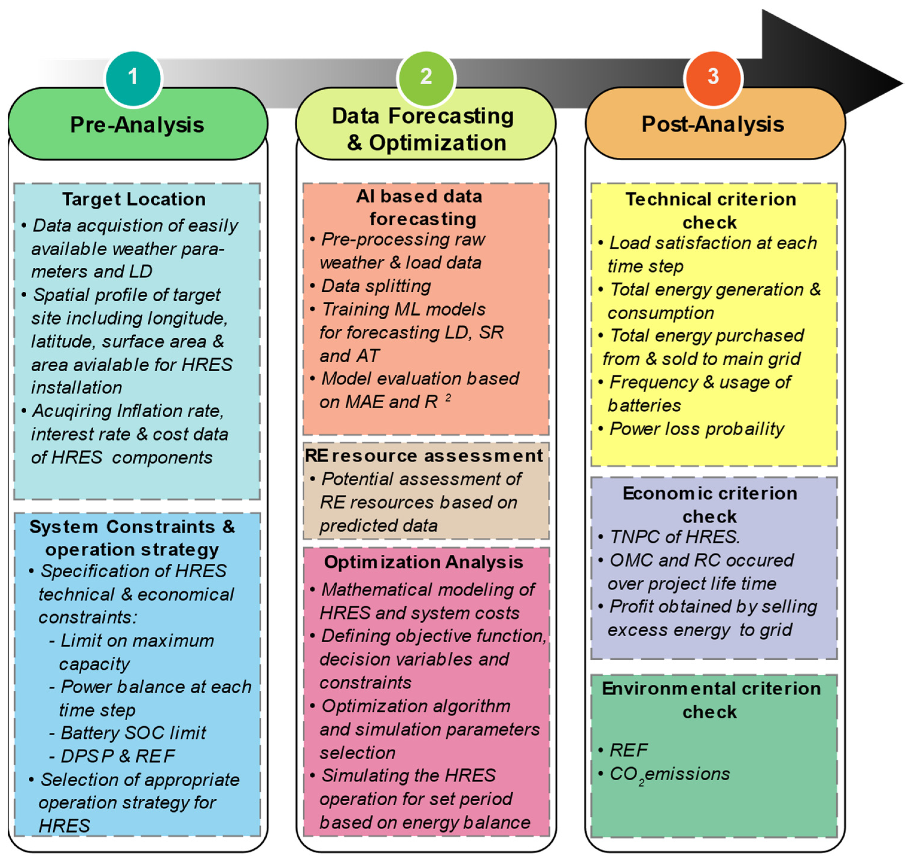
2. Materials and Methods

A grid-connected hybrid PV and battery energy system was proposed to satisfy the LD of a typical commercial building in an urban area. A techno-economic analysis followed by optimal size selection for the proposed system was conducted, followed by a sensitivity analysis to investigate the influence of variations in the techno-economic constraints and parameters of the HRES on the optimization results. Figure 1 shows the three stages of the methodology adopted in this study to obtain the optimum sizing of the HRES while satisfying all the constraints.

The first stage is the pre-analysis, which mainly deals with acquiring input data, specifying the constraints and deciding on the appropriate operational strategy required in designing and operating the HRES. The input data primarily consist of weather parameters, the LD profile, area availability, the costs of HRES components and the inflation and interest rates of the selected location. Additional required inputs relate to the specification of constraints associated with system sizing and operation, including the component size limits, power balance, limits on the battery state of charge (SOC), allowed renewable energy fraction (REF) and deficiency of renewable power supply probability (DRPSP). In the data forecasting and optimization stage, ML ensemble models are developed to forecast the input variables required to simulate the HRES, and the forecasting accuracy is evaluated based on widely used performance metrics. The detailed ML framework development and evaluation procedure are presented in Section 2.3. As a final step in this stage, HM optimization algorithms are used to minimize the total net present cost (TNPC) of the HRES as a function of decision variables—the numbers of PV panels and battery packs—while satisfying all stated constraints. Lastly, post-processing and visualization of the optimization results are carried out in the post-analysis stage. The set objectives based on technical, economic and environmental factors are evaluated, including checking the system reliability, total production and consumption, power supply reliability, frequency of battery usage and main grid interactions, as well as a cost analysis of the optimum system and the CO₂ emissions associated with the selected system.

2.1. Problem Statement and Objective of Study

Most studies on the optimal sizing of HRES simulate the proposed system for a 1-year duration and extend the results into the future for a duration equivalent to the system lifespan. This projection is based on the assumption that the weather and LD patterns will remain somewhat consistent. Furthermore, this method is employed primarily due to the difficulties in acquiring input data for longer durations, associated measurement costs and high computational effort. However, with the advent of AI-based data-driven approaches, long-term data forecasts can be made without additional cost overheads related to data acquisition. Moreover, the sizing problem is not a dynamic optimization problem and, thus, the high computational effort is a reasonable non-recurrent price to pay to obtain greater economic benefits over the long term. Therefore, the main objective of this study is to investigate the effect of simulating the proposed HRES over its lifetime, compared to a 1-year simulation based on ML data forecasts. The proposed HRES is composed of a PV power plant and battery storage as a backup power supply unit and is connected to the main grid, as shown in Figure 2. The goal here is to validate the theory that simulating and optimizing the system size based on its whole lifetime results in a more physically accurate result, although it may lead to a higher TNPC value.

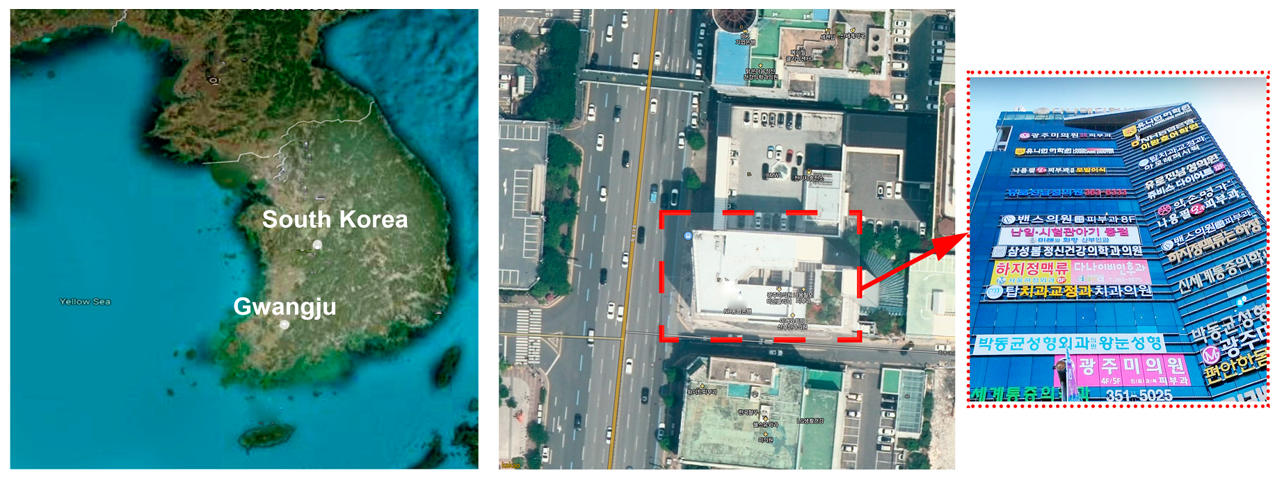
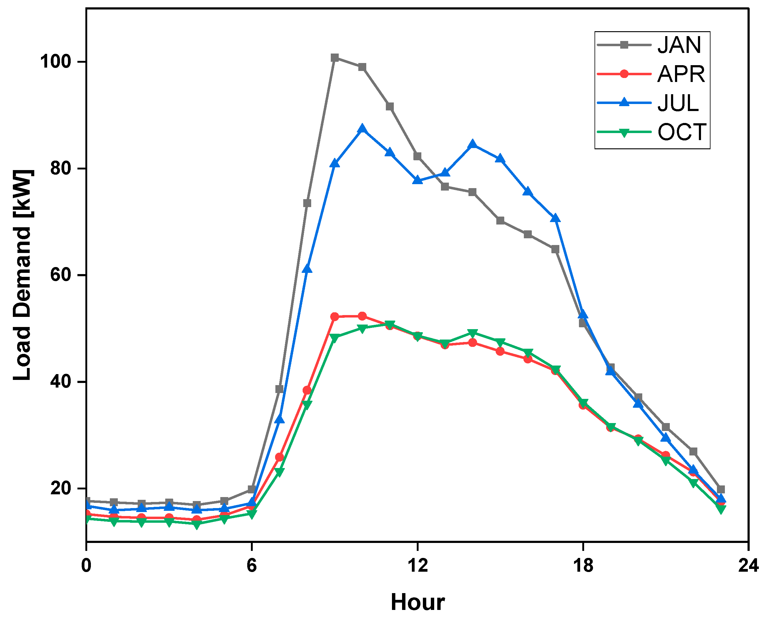
2.2. Description of the Target Location

The proposed methodology has been implemented for a commercial center in Gwangju, South Korea, connected to the main electrical grid. The load demand data for the analysis were acquired for this commercial center from the Korean Open Data Portal [40] and the building structure and location are shown in Figure 3. The monthly average of the daily load profile for the four months of January, April, July and October, representing the four seasons, is shown in Figure 4. As shown, the maximum load (90–100 kW) occurs in January and July (winter and summer seasons), while, for April and October (spring and fall seasons), the peak LD is about half of the yearly maximum as the weather becomes milder. The hourly analysis reveals that the LD is about 20 kW at 6:00 in the morning as the day starts and continuously increases up to almost 100 kW by 10:00 and remains almost constant for the next 6 h; it then decreases again after the business closes for the day. The fact that the LD remains almost constant at about 50 kW for the spring and fall seasons, while this number almost doubles for the summer and winter seasons, shows that the weather variations directly influence the electrical energy consumption behavior.

The renewable energy resources were evaluated at this location and the analysis revealed an abundance of solar radiation (maximum value of 0.7 MJm⁻²) but a scarcity of good wind speeds (mean value of 2 ms⁻¹). Based on these findings, we conclude that implementing a wind turbine energy system under the local wind speed conditions would not be economically viable. Additionally, as a component of our optimization algorithm, we also analyzed the optimization of the wind turbine capacity for the selected location. The outcome of this analysis revealed a near-zero value, reinforcing the conclusion that the exploitation of wind energy is not a viable option at this location. The solar resource at the target location is highly intermittent, leading to very complicated design problems in obtaining the optimum size of the HRES system. In the next section, we use ML models to predict the input variables required to optimize the HRES capacity.

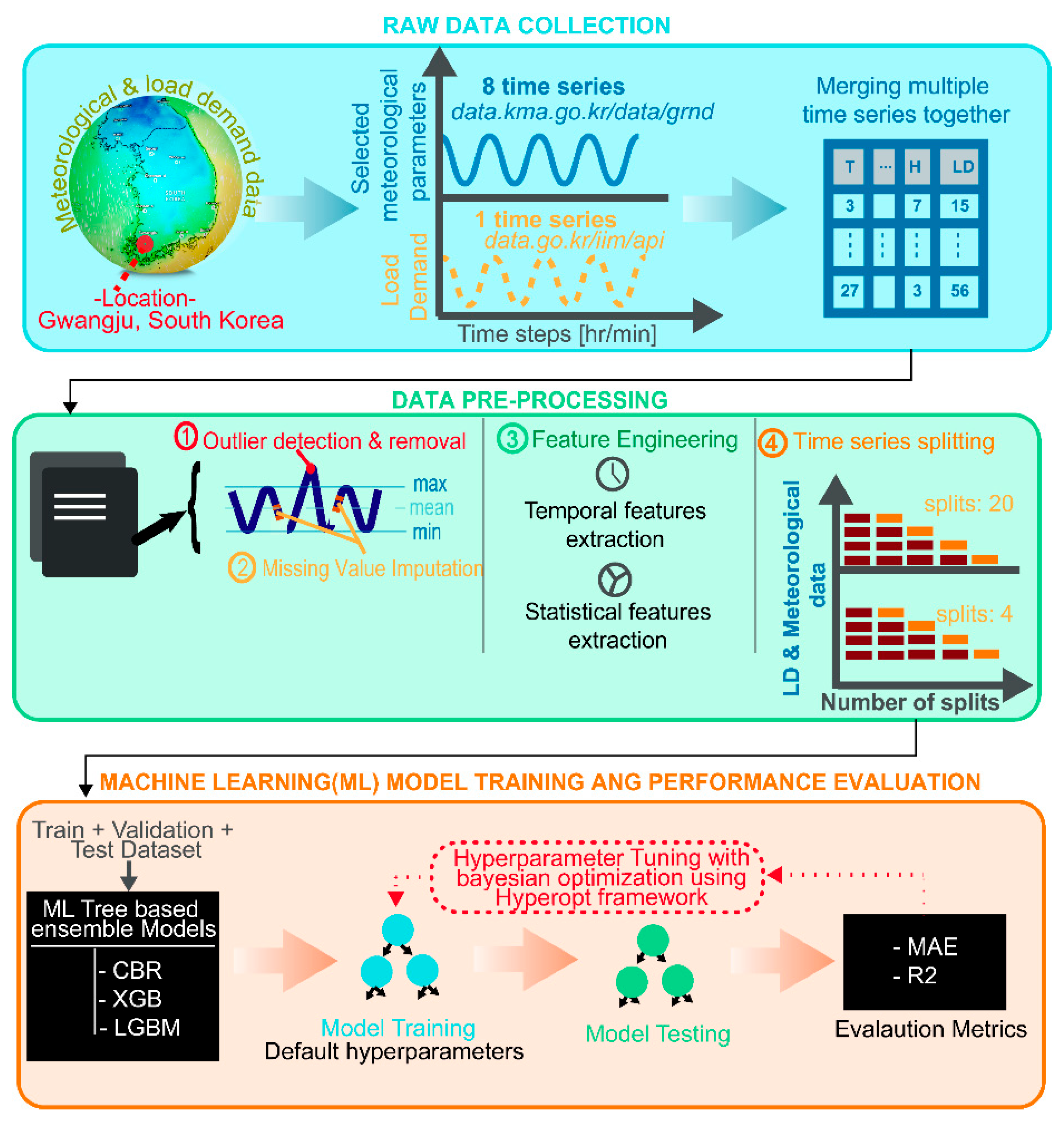
2.3. Machine Learning Framework

In this study, we developed a machine learning framework to forecast three target variables, solar radiation, air temperature and load demand, as shown in Figure 5. The framework consists of the following key steps: data acquisition; pre-processing; feature engineering; the training of machine learning models, including the cat boost regressor (CBR), extreme gradient boosting (XGB) and light gradient boosting machine (LGBM); hyperparameter tuning; and model performance evaluation using the coefficient of determination R2 and MAE. The three models were trained and evaluated for each target variable, leading to a total of nine models. In the following sections, we provide more details on each of these steps and how they contribute to the overall performance of the machine learning approach.

2.3.1. Data Collection

Two different time series datasets, recorded at different temporal resolutions, were used for the forecasting of the target variables as a function of the meteorological parameters for the selected location. The publicly available meteorological dataset was obtained from the Korean Meteorological Association (KMA) [41], while the load demand dataset was obtained from the Korean government’s Open Data Portal [40]. The former dataset was collected over 35 years (1980–2015), while the latter was recorded for two years.

Table 1. Description of two datasets used in the study.

Dataset	Raw Data Variables	Missing Data (%)	Temporal Resolution	Input Variables	Target Variable
Meteorological data	AT [C]	4.16	1 h	AT GT H Pr WS WD TC SS	SR AT
	H [%]	26.17
	GT [C]
	Pr [mm]	88.81
	WS [m/s]	0.04
	WD [deg]	0.04
	TC
	SS [h]
	SR [MJ/m2]
Electric power consumption data	LD [kW]	4.10	15 min	SR SS	LD

AT: air temperature, H: relative humidity, Gt: ground temperature, Pr: precipitation, WS: wind speed, WD: wind direction, TC: total cloud, SS: sunshine duration, SR: solar radiation.

presents detailed information about these datasets, including raw data variables, missing data percentages, temporal resolution and input and target variables associated with weather and load demand forecasting.

2.3.2. Data Pre-Processing

Data pre-processing is an integral part of the overall ML pipeline, which allows for identifying and transforming any anomaly in the raw dataset. In the present study, the exploratory data analysis of the two input datasets revealed a notable percentage of missing values in the relative humidity and precipitation data, as shown in Table 1. The missing values in the meteorological parameters were dealt with after examining the data recording procedures outlined by the KMA, which state that the absence of precipitation (Pr) variables indicates unmeasurable precipitation in the atmosphere. The null values in solar radiation (SR) and sunshine (SS) corresponded to nighttime and the missing data in temperature (T), relative humidity (H), wind speed (WS), wind direction (WD) and LD variables were associated with equipment failures. Missing values in Pr, SR and SS variables were set to zero, while cubic interpolation was used for other missing values, and no missing values were found in the total cloudiness (TC) variable.

Three types of features were engineered from the basic input variables: temporal, statistical and domain features. The first category includes features such as the hour of the day, day of the year, hour angle, cosine transformed day of the year, time difference (TD) features and time lags of temperature and TD-derived features. The TD feature was calculated based on the original SR variable, resulting in a new feature called solar radiation change (SRC), which is essentially the difference between the SR at the current time step (t) and its first-time lag SR (t − 1) [42]. Statistical features such as the rolling and expanding mean were derived from the basic variables T, H and SR and the following two domain features were generated: the dew point temperature (DPT) and the variable corresponding to the ratio of the ground temperature (GT) to DPT, where the DPT was formulated from basic variables, the air temperature (AT) and H.

After the feature engineering step, three different datasets were finalized, each for the prediction of a different target variable, and details about these datasets are presented in

Table A1. Data pre-processing details.

Prediction Target	Input Features
	Basic Variables	Timestamp Derived Variables	Time Difference and Lag Variables	Statistical Variables
SR	AT H WS WD SS TC	Hour of day	SRC(t) SRC(t − 1) SRC(t − 2)	-
AT	GT AT H	Hour of day	AT(t − 1) AT(t − 2) AT(t − 3)	GT/DPT Rolling mean of T
LD	AT H Pr	Hour of day Day of year Hour angle	-	SR expanding mean, H expanding mean, Cosine (day of year)

in Appendix A. The resulting datasets were first separated into training and test sets such that the test set covered the last 15 years of input data (equivalent to the project lifetime of the proposed HRES). To improve the models’ training and validation accuracy, the models were cross-validated based on Keras time series cross-validation. Two datasets were generated for each split: a training set for model learning and a validation set to optimize the models. Additionally, the test dataset was used in evaluating the generalization capability of the trained and optimized models. The number of splits in this cross-validation setup was considered an important hyperparameter and was optimized for each input dataset as a part of the ML model building process, as also shown in Figure 5.

2.3.3. Machine Learning Algorithms, Hyperparameter Tuning and Performance Evaluation

Ensemble learning in the ML domain refers to methods combining multiple base models to predict or classify the target variable based on the idea that a prediction error in a single model forecast may be compensated by the other models. These methods can be classified into two main categories, dependent and independent methods, where, in the former category, the new base model is guided in the learning process based on knowledge learned in the previous base model, whereas, in the latter, the learning of each base model is completely independent. One of the dependent ensemble methods involves a model learning process where the objective is to construct new base learners based on optimizing the whole ensemble loss function [43,44]. In the current study, three advanced gradient boosting machine (GBM) models (XGB [45], LGBM [46] and CBR [47]) are selected for multivariate time series forecasting. These models are built upon a GBM base structure with better feature splitting, optimized parallel learning, enhanced gradient boosting and reduced memory and computation requirements [48].

Over the last few years, compared to deep sequence models, these GBM models have extensively been used in time series forecasting applications such as stock prediction, gold price prediction, waste frequency prediction and predicting the relationship between the weather and the COVID-19 [49]. These ensemble methods have an advantage over the DL models based on their better interpretability, higher computational efficiency and relatively better performance but require extensive hyperparameter tuning. A popular hyperopt framework is used to tune all the hyperparameters of these models for each target variable and associated dataset [50]. In this study, Tree of Parzen Estimators was selected as an optimization algorithm for each hyperparameter study, and the number of iterations was set to 200. The generalization capability of all the models was evaluated based on two popular statistical measures: MAE and R2. The mathematical expressions for the calculation of these metrics are presented in

Table 2. ML models’ performance evaluation metrics.

Performance Metric	Mathematical Expression
MAE	${\displaystyle \sum _{j=1}^n}{\left|A_j-P_j\right|}^2$
R2	$1-\frac{{{\displaystyle \sum }}_{j=1}^n{\left|A_j-P_j\right|}^2}{{{\displaystyle \sum }}_{j=1}^n{\left|A_j-A_{mean}\right|}^2}$

MAE: mean absolute error, R2: coefficient of determination.

, where variable A represents the actual observation and variable P the predicted value. Furthermore, AI-based solutions may be verified to be accurate and error-free using formal approaches [51]. These procedures entail the application of mathematical approaches to ensure that the software implementation adheres to the formal specifications. By doing this, even when working with complicated and ambiguous data, we can ensure that the AI-based system acts as intended and yields accurate results [52].

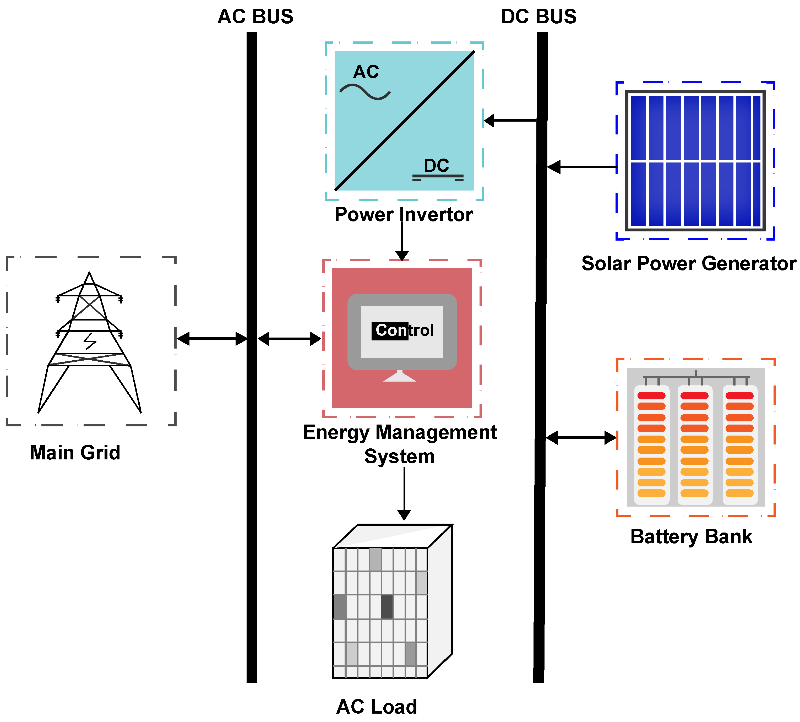
3. Mathematical Modeling of Renewable Energy System Components

3.1. PV System Model

The total electric power generated from a PV array is modeled by Equation (1) as a function of the solar radiation incident on the tilted PV surface ($S{R}_{tilt}$), the area of the PV panel ($A$) and the overall efficiency of the PV module (${\eta }_{PV}$). The technical and cost data of the selected PV module are presented in

Table 3. Technical and economic parameters of PV module.

PV MODULE
Technical Specifications
Manufacturer	Hanwha
Cell Type	Q Cell
Surface Area (m2)	1.7943
Rated Power (W)	360
Short-Circuit Current (Amp.)	11.04
Open-Circuit Voltage (V)	41.18
Module Efficiency (%)	20.1
Temperature Coefficient of Rated Power (%/K)	−0.34
Nominal Cell Operating Temperature (K)	316
Cost Data
Capital Investment ($/W)	1.5
Replacement Cost ($/W)	1.2
Operation and Maintenance ($/W/year)	0.03
Life (years)	25

[53]. This base model, however, does not consider any of the power losses associated with the real-time operation of a PV system over its lifespan, such as losses incurred due to increased cell temperatures, dust and snow accumulation, panel soiling, wiring heat losses and age-based performance deterioration. However, the techno-economic feasibility of a PV array system’s real-life implementation requires that such losses be incorporated for a more physically accurate representation of the system. The influence of these detrimental factors is incorporated into the base model (Equation (1)) by re-defining the overall PV module efficiency given in Equations (1)–(5) [54].

$$P_{PV}=S{R}_{tilt}\ast A\ast {\eta }_{PV}$$

(1)

P_PV (kW) corresponds to the power generated from a single PV panel. The ${\eta }_{PV}$is then modified such that it includes the PV panel efficiency under standard temperature conditions (${\eta }_{STC}$) and the loss in PV power due to higher cell temperatures (${\eta }_{temp}$), and the degradation factor (${\eta }_{degradation}$) is assumed to be 80% [55].

$${\eta }_{PV}={\eta }_{STC} \ast {\eta }_{temp} \ast {\eta }_{degradation}$$

(2)

$${\eta }_{STC}=\frac{S{R}_{PV}}{S{R}_{STC}}$$

(3)

$S{R}_{PV}$ denotes solar radiation on PV modules, while $S{R}_{STC}$ is the solar constant with a value of 1 kWm⁻².

$${\eta }_{temp}=1-\alpha \left(T_c-T_{c_{STC}}\right)$$

(4)

The variables $T_c$(°C) and $\alpha \left(\frac{\%}{°\mathrm{C}}\right)$refer to the PV cell temperature and temperature coefficient, respectively. The variable $T_{c_{STC}}$ represents the standard cell temperature under standard temperature conditions. The cell temperature is mathematically formulated as in Equation (5):

$$T_c=T_a+SR\ast \frac{NOCT-20}{800}$$

(5)

$T_a$(°C) and $NOCT$(°C) represent ambient air and the nominal cell temperature. Additionally, the total solar power generated by an array of N_PV panels can be obtained via the expression presented in Equation (6):

$$Total P_{PV}=P_{PV} \ast N_{PV}$$

(6)

where P_PV (kW) is the power generated from a single PV panel.

3.2. Battery ESS Model

Battery ESS acts as a backup power supply unit in the event that the total LD cannot be fulfilled by the HRES alone and as a storage unit when the LD is less than the total renewable energy production and surplus energy is charged into the battery system. The intermittency of SR resources leads to fluctuations in renewable energy production, which highlights the significance of the battery energy management system (BEMS). Depending upon the net state of total renewable energy generation (TREG) and LD, the BEMS operates in two modes: charging and discharging. The charging power $E_{ch}\left(kW\right)$ is fed into the battery ESS when $E_{TREG}>E_L$and the battery ESS is discharged with power $E_{dh}\left(kW\right)$ when $E_L>E_{TREG}$. The technical specifications of the battery mentioned in

Table 4. Technical and economic parameters of battery module.

Battery
Technical Specifications
Manufacturer	Rolls/Surrette
Type	Surrette 6CS25P
Maximum Capacity (Ah)	1150
Capacity (Ah)	820
Rated Voltage (V)	6
Rated Current (Amp.)	152
Charge/Discharge Efficiency (%)	89.4
Round Trip Efficiency (%)	80
Cost Data
Capital Investment ($/W)	0.25
Replacement Cost ($/W)	0.25
Operation and Maintenance ($/W/year)	0.001
Life (years)	20

are utilized to calculate the charge and discharge energy of the battery ESS, using the mathematical model described by Equations (7)–(9) [56].

$$E_{ch}\left(t\right)=\left[E_{TREG}\left(t\right)-\left(\frac{E_L\left(t\right)}{{\eta }_{\frac{DC}{AC}} }\right)\right]\ast {\eta }_{ch}$$

(7)

$$E_{dh}\left(t\right)=\left[\left(\frac{E_L\left(t\right)}{{\eta }_{\frac{DC}{AC}} }\right)-E_{TREG}\left(t\right)\right]/{\eta }_{dh}$$

(8)

$$P_{BAT}\left(t\right)=E_{ch}\left(t\right)=-E_{dh}\left(t\right)$$

(9)

The energy available in the battery ESS at time t depends on the charging and discharging power of the ESS, which varies under the influence of $E_L\left(\mathrm{kWh}\right)$, the energy equivalent of LD at time t, and $E_{TREG}\left(\mathrm{kWh}\right)$, the total renewable energy generated at time t. The energy stored in a battery is usually represented by the SOC as given in Equations (10) and (11), respectively [24].

$$SO{C}_{batt}^{ch}\left(t\right)=SO{C}_{batt}\left(t-1\right)\ast \left(1-\sigma \right)+E_{ch}\left(t\right)$$

(10)

$$SO{C}_{batt}^{dh}\left(t\right)=SO{C}_{batt}\left(t-1\right)\ast \left(1-\sigma \right)-E_{dh}\left(t\right)$$

(11)

where $SO{C}_{batt}^{ch}\left(t\right)$ is the battery ESS energy available at time t during charging and $SO{C}_{batt}^{dh}\left(t\right)$ is the battery ESS energy available at time t during discharging. $SO{C}_{batt}\left(t-1\right)$ is the energy state of the battery ESS at time t − 1 and $\sigma$ is the self-discharge rate of the battery, which is used to incorporate the battery energy losses when it is not being used.

3.3. Inverter Model

A power inverter transforms the voltage and current from electronic devices operating on a DC configuration into a corresponding AC, and, in a typical HRES, it controls the power flow between the DC and AC components of the HRES. This device’s primary function is converting the DC voltage produced by the PV array and battery ESS into AC to satisfy the AC LD and its optimal size directly depends upon the total renewable energy production and maximum throughput of the battery ESS. The size of the inverter should be greater than the TREG and maximum throughput of the battery ESS to ensure the safe operation of these inverters [57]. In this study, the inverter is oversized by 20% based on its optimal size. Moreover, power losses related to the operation of such devices are also incorporated into the mathematical model described by Equation (12) [58]:

$$C_{PI}\ge \frac{1.2\ast \left({\eta }_{\frac{DC}{AC}} \left(\max \left(P_{PV}\right)+\max \left(T{P}_{BESS}\right)\right)\right)}{P_{R_{INV}}}$$

(12)

where C_PI represents the final capacity of the power inverter, TP_BESS is the energy throughput of the battery ESS, η_(DC/AC) is the inverter efficiency and $P_{R_{INV}}$indicates the rated power of the inverter. The techno-economic input parameters for the PI module selected are presented in

Table 5. Technical and economic parameters of inverter module.

Inverter
Technical Specifications
Manufacturer	LEONICS
Type	MTP-413F 25 kW
Rated Power (kW)	25
Maximum Input voltage (V)	240
Rated Voltage (V)	240 DC
Rated Current (Amp.)	72
Maximum efficiency (%)	95
Cost Data
Capital Investment ($/W)	0.8
Replacement Cost ($/W)	0.8
Operation and Maintenance ($/kW/year)	0.01
Life (years)	10

[51].

3.4. Grid Interaction Model

The power from the main grid is modeled as a nearly infinite source, assumed always to satisfy the LD, and is described by Equation (13). The electricity unit price for energy purchase from the main electric grid was 0.07 $/kWh and the grid sellback price to the main grid was 0.098 $/kWh, taken from the Korean Electric Power Company and Korean Power Exchange, respectively [59,60]. Generally, the unit price for energy purchase from the grid is higher than the unit price at which any surplus energy is sold to the grid. However, in this study, considering the Korean government’s subsidies on renewable energy buy-back, the selling price was set higher than the purchasing price.

$$P_{grid}=99,999 \left(\mathrm{kW}\right)$$

(13)

where $P_{grid}$ refers to the available electric power from the main grid.

3.5. Techno-Enviro-Economic Performance Evaluation Criteria

The capacity of the proposed HRES is optimized based only on the TNPC of the system; however, other technical criteria, including power supply reliability and allowed renewable energy (RE) supplied to the energy system, are incorporated into the optimization process as system constraints. Additionally, the selected system’s environmental impact is evaluated based on the net CO₂ emissions of the optimized HRES. TNPC is the total cost of the HRES incurred over the project lifetime, which is the cumulative sum of the initial cost, operation maintenance cost (OMC) and replacement cost (RC) and is mathematically formulated as in Equation (14) [61]:

$$TNPC=IC+OMC+RC$$

(14)

OMC and RC are the recurring and non-recurring costs calculated by Equations (15) and (16), respectively:

$$OMC=OM{C}_i·\left(\frac{1+inf}{int-inf}\right)·\left(1-{\left(\frac{1+inf}{1+int}\right)}^{P_L}\right)$$

(15)

$$RC={{\displaystyle \sum }}_{i=1}^{n_r}\left(N_r·R{C}_{unit}·{\left(\frac{1+inf}{1+int}\right)}^{\left(\frac{P_L·i}{n_r+1} \right)}\right)$$

(16)

where $OM{C}_i$ is the annual OMC for the starting year, $inf$ is the inflation rate taken as an average value of 5.71% [62], $int$is the real interest rate taken as 3.26% [63], $P_L$is the project lifetime, $n_r$is the frequency of component replacement during $P_L$, $N_r$ is the number of HRES components to replace and $R{C}_{unit}$ is the per unit replacement cost.

The power supply reliability of only the renewable energy system (RES) is represented by the DRPSP value, which indicates the likelihood that the energy coming only from the renewable energy system will not be able to satisfy the required LD for a time period of T and is given by Equation (17) [64].

$$DRPSP=\frac{{{\displaystyle \sum }}_{t=1}^{T}LD\left(t\right)-E_{HRES}\left(t\right)}{{{\displaystyle \sum }}_{t=1}^{T}LD\left(t\right)}$$

(17)

where $E_{HRES}\left(t\right)$ is the total energy supplied by the HRES at time t in kWh per year. The percentage of the total energy produced by RE resources, including all the battery interactions and surplus generation to satisfy the total LD, is represented by the REF and is defined as Equation (18) [65]. The DRPSP metric is focused on the reliability of the system, while the REF metric is focused on the contribution of the renewable energy sources in meeting the energy demand.

$$REF=\left(\frac{{{\displaystyle \sum }}_{t=1}^{T}L{D}_{TREG}\left(t\right)}{{{\displaystyle \sum }}_{t=1}^{T}LD\left(t\right)}\right)·100$$

(18)

Environmental factors associated with HRES have become a crucial part of their performance evaluation, indicating the amount of greenhouse gas (GHG) emissions produced by such systems. Generally, HRES comprising only RE resources produce almost no emissions during HRES operation. However, such systems are connected to the main grid and a notable percentage of GHG emissions are released, including CO₂, which can be calculated as a function of the energy produced by non-renewable resources per MWh and associated CO₂ emissions produced per tonnage, as presented in Equation (19) [64].

$${CO}_2={\displaystyle \sum _{t=1}^T}{\displaystyle \sum _{n=1}^N}{E}_n·TEP{N}_{n,t}$$

(19)

where $E_n$ (ton/MWh) corresponds to the emissions of CO₂ from an energy generation unit of type n. $TEP{N}_{n,t}$ (MWh) is the total energy produced by non-renewable energy generating unit type n for time t, which in this case is all the energy purchased from the main electric grid.

3.6. Hybrid Optimization Algorithms

This study employs a comprehensive optimization process for the optimal sizing of the HRES utilizing nine different optimization algorithms, including six hybrid and three simple algorithms to evaluate the cost objective function (OF). The hybrid algorithms are the hybrid firefly–particle swarm optimization algorithm (HFPSO) [66], the constriction-coefficient-based particle swarm optimization–gravitational search algorithm (CPSOGSA) [67], the hybrid particle swarm optimization–butterfly optimization algorithm (HPSOBOA) [68], the hybrid augmented grey wolf optimization–cuckoo search algorithm (AGWOCS) [69], the hybrid elephant herding optimization (EHOTOPSIS) [70] and the hybrid sperm swarm optimization–gravitational search algorithm (HSSOGSA) [71]. The remaining three algorithms are the hybrid stochastic fractal search–fitness distance balance (FDBSFS), which incorporates a new fitness–distance balance (FDB) selection strategy [72], the hybrid teaching–learning-based artificial bee colony algorithm (FDBTLABC) [73] and the hybrid manta ray foraging optimization algorithm with dynamic fitness distance balance (dFDBMRFO), which modifies the traditional FDB with a dynamic distance factor such that a new selection strategy dynamic, FDB (dFDB), is introduced [74]; these are non-hybrid algorithms but employ novel particle selection methods in their core algorithms for better performance. Generally, the working of any optimization algorithm can be described by three main steps, which are repeated until the maximum number of iterations is reached. These steps include the initialization of search agents, the mechanism of exploring the search space via these agents and finally updating the positions of these search agents to a new location. All of the implemented algorithms except HPSOBOA randomly initialize the search agents, while HPSOBOA employs a 1D cubic map that generates a uniformly distributed random number sequence, which is used to initialize the search agents. A detailed explanation of each algorithm can be found in

Table 6. Detailed descriptions of implemented metaheuristic optimization algorithms.

Algorithm Name	Search Process	New Position Update
HFPSO	After initialization, the algorithm starts with a global search using the PSO algorithm, which provides fast convergence in exploration. Then, the firefly algorithm is used for a local search to avoid becoming trapped in local minima. The light attraction of each particle is mutated by a PSO operator to balance exploration and exploitation. This process helps to increase the particle diversity and achieve a faster convergence ability in the hybrid HFPSO algorithm.	After the search process, if a particle’s fitness value is more than or equal to the previous global best, it is anticipated that a local search will begin and a new position will be calculated by an imitative FA; otherwise, the particle will be handled by PSO, which will carry on with its regular operations with this particle.
CPSOGSA	PSO uses a combination of its velocity and position update equations, along with the inertia weight and constriction coefficient, to exploit new regions of the search space. The coefficient ensures that the search agents do not move far away from the promising local regions of the search space. GSA contributes to exploitation by using gravitational forces between agents to converge towards the global optimum.	The positions of particles are updated based on the current position and velocity calculated by a new equation, which is constructed by merging the velocity equation of GSA in the PSO equation.
HPSOBOA	PSO is used to update particle velocities (global exploration), while BOA is used to update positions and perform local search by allowing each particle to explore its immediate neighborhood in detail by use of an adaptive parameter.	BOA uses a probabilistic model to generate a new position for each dimension of each particle’s position vector based on its previous values and those of other particles in its neighbor, and the process continues until maximum iterations.
AGWOCS	Performs global search using AGWO by updating the positions of wolves based on its augmented position update equation, facilitating faster exploration by allowing wolves to jump at random positions throughout search space. Local search is carried out by CS for efficiency by using Levy flights.	After local search is done, the optimal positions of some wolves as found in AGWO are updated by CS results and the final positions are achieved and are evaluated for OF. If there is no improvement in the OF value, the whole process starts again till maximum iterations are reached.
EHOTOPSIS	IEHO generates a population of elephants and updates their positions in the exploration phase by moving them toward their best positions found so far. It promotes diversity by replacing the worst elephant with a new baby elephant. The exploitation phase selects promising solutions and updates them to move toward better solutions with small variations to promote diversity.	Best and worst elephant position is updated based on local search, while all other elephants are positioned based on their neighbors (output of global search).
HSSOGSA	The GSA assigns masses to solutions and calculates gravitational force to explore new regions. SSO exploits promising regions by simulating a sperm swarm that moves toward promising solutions. The algorithm updates its population based on the selected solutions.	HSSOGSA uses a weighted sum approach to combine the positions updated by GSA and SSO. The weights are determined by a parameter called the “exploration factor,” which controls the balance between exploration and exploitation before calculating new Pbest and GBest.
FDBSFS	In the exploration phase, a Gaussian Walk method generates new particles from diffusion applied to all points in the population. The exploitation phase selects particles based on fitness and distances from each other using the FDB method, which balances both factors by sorting and penalizing close particles.	The selected particles are then updated using a velocity equation that considers their current position, their best position so far and the best position of all particles in the population, which helps to refine existing solutions by moving particles toward better positions in the search space.
FDBTLABC	The ABC algorithm uses learning-based onlooker and generalized oppositional scout bee stages for exploration, while the teaching-based bee stage is used for exploitation. Onlooker bees choose a solution based on probability, while scout bees generate new solutions. Teacher bees improve the quality of solutions by sharing their knowledge.	The algorithm updates bee positions via a greedy selection method. Bees generate new solutions by modifying their positions based on a bee selected at random. The best solution replaces the current best if it has a better fitness value. The employed and onlooker bee stages use teaching and learning mechanisms, respectively.

.

The main goals of the hybridization of algorithms include the achievement of improved convergence and stability of results, especially when the search space becomes complex. Most of the algorithms implemented in this study are constructed by merging two simple metaheuristics such that the enhanced exploitation characteristics of one are complemented by the enhanced exploration characteristics of the other. Few algorithms have utilized the FDB selection strategy and its variants for the filtering out of the poor solutions to further enhance the search process of the algorithm. Although each implemented algorithm in this study possesses different characteristics, the outcomes of the unique characteristics in each algorithm can simply be measured in terms of their convergence characteristics, the required number of iterations and the stability of results. In the present study, such a comparison of all the implemented algorithms was conducted and the results are presented in Section 4.2.

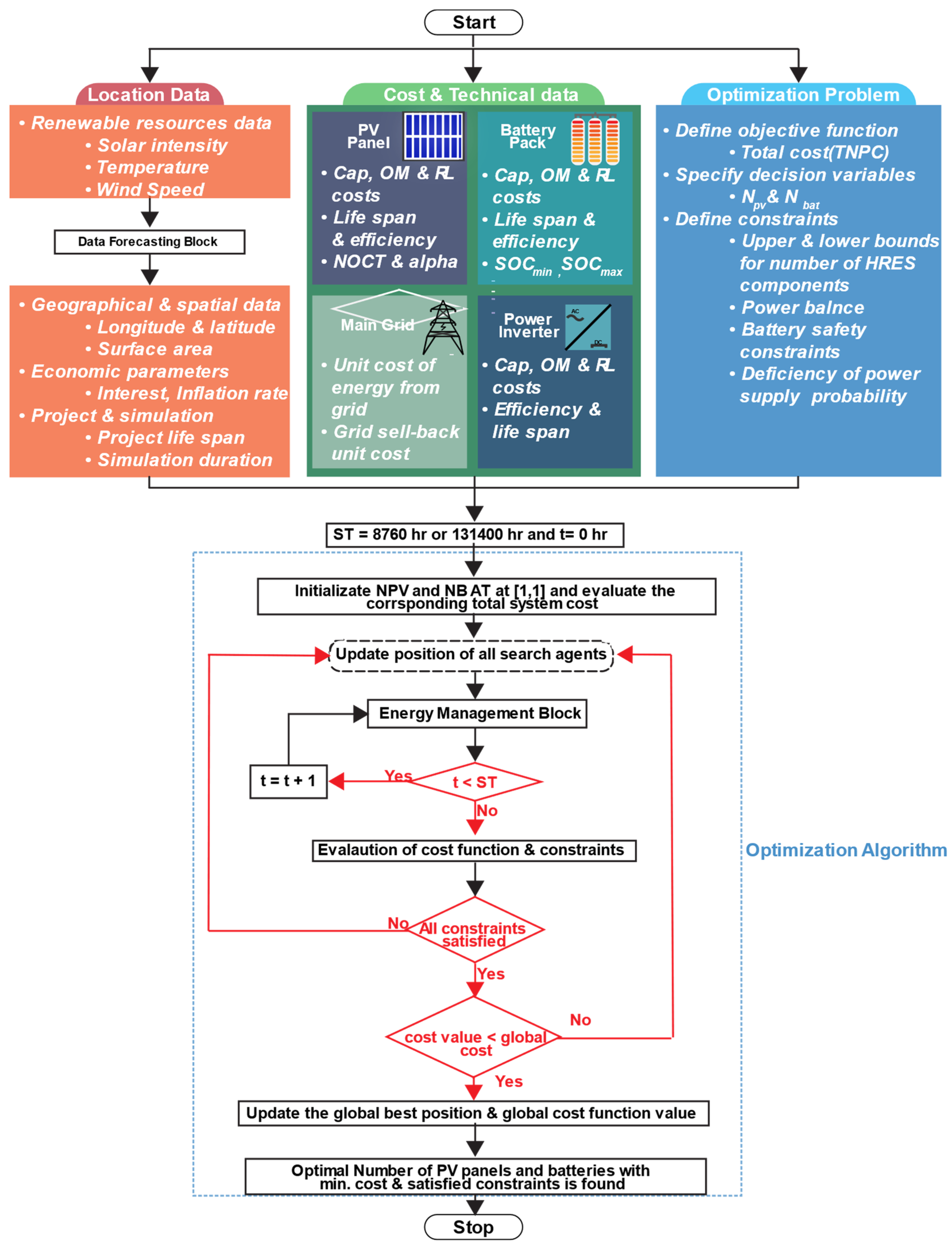
3.7. Optimization Problem Formulation

In this study, a capacity optimization problem was formulated to minimize the TNPC with the smallest DRPSP of the proposed energy system. The goal was to find the HRES configuration that would lead to the minimum TNPC and also satisfy all the system constraints, including DRPSP. The flowchart in Figure 6 illustrates the capacity optimization procedure that was adopted in this study, and the mathematical formulation of the optimization process is described in Equations (20)–(26).

Objective Function:

$$Minimize:TNPC=f\left(N_{PV},N_{BAT}\right)$$

(20)

Decision Variables:

$$Number of HRES components:N_{PV},N_{BAT}$$

The optimization constraints include the power balance constraint, minimum and maximum allowed capacity of HRES components, battery ESS safety, system power reliability and required REF. The HRES power balance constraint at time t is given by Equation (21).

$$P_{PV}\pm P_{BAT}\pm P_{grid}=LD$$

(21)

The sign convention used here is based on the direction of energy flow, where positive and negative values indicate energy flowing in and out of the system, respectively.

The minimum and maximum allowed number of HRES components, including the numbers of PV panels N_PV and batteries N_BAT, are given by Equation (22).

$$\left\{\begin{array}{c}{N}_{P{V}_{min}}\le N_{PV}\le N_{P{V}_{max}}\\ N_{BA{T}_{min}}\le N_{BAT}\le N_{BA{T}_{max}}\end{array}\right.$$

(22)

The battery SOC should be maintained within specified limits set by the manufacturer for efficient operation and a prolonged lifetime, as mentioned in Equation (23).

$$SO{C}_{BA{T}_{min}}\le SO{C}_{BAT} \left(t\right)\le SO{C}_{BA{T}_{max}}$$

(23)

$SO{C}_{BA{T}_{min}}$ is calculated as a function of the maximum allowed depth of discharge (DOD) and the battery’s nominal capacity. Generally, the battery manufacturers specify the optimal value of DOD, which in this case is 70% [75].

$$SO{C}_{BA{T}_{min}}=\left(1-DOD\right)\ast BA{T}_{nominal}$$

(24)

where $BA{T}_{nominal}$ is the nominal capacity of the battery, which is equal to $SO{C}_{BA{T}_{max}}$.

The power supply reliability of RES is ensured by considering a DRPSP value that should be less than a specified limit, as given by Equation (25).

$$DRSP{S}_{optimized}\le DRSP{S}_{max}$$

(25)

In a typical grid-connected HRES, the renewable fraction provides a means to observe and control the amount of electrical power production that comes from renewable resources, as presented by Equation (26).

$$REF\ge RE{F}_{max}$$

(26)

where $RE{F}_{max}$ refers to the maximum allowable limit of the renewable energy fraction in the entire system, which is set to a constant value of 30%, considering the available space constraints of the building considered in this study.

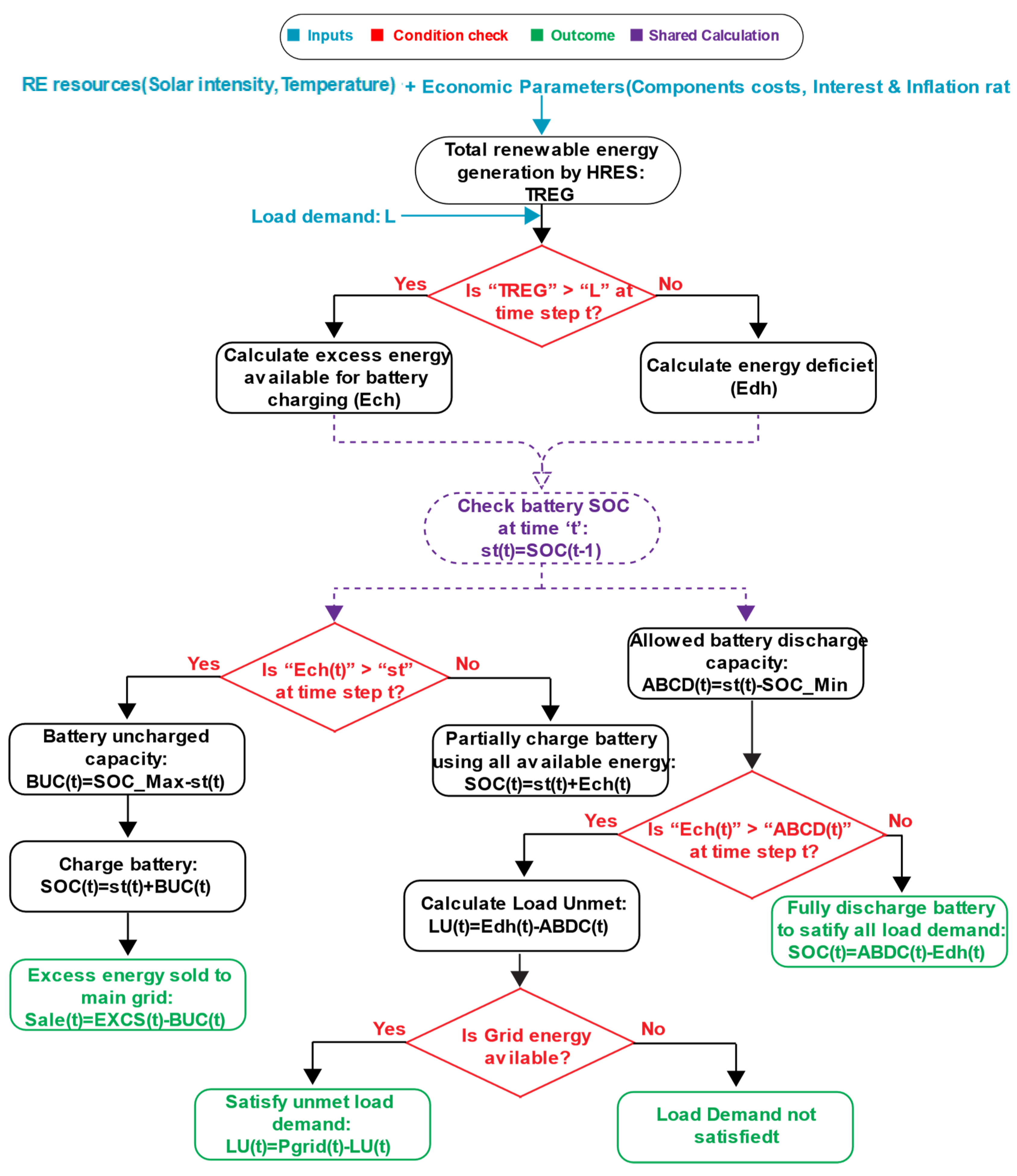
3.8. Energy Management Strategy

A rule-based energy management strategy is developed to control the energy flow through different components of the HRES optimally, as shown in Figure 7. The optimal dispatch of HRES components as part of energy management starts with quantifying the total energy generated by the HRES and the total LD over a specified time period. Based on the difference between the energy supplied and LD, two scenarios can occur at any time step t:

1.

When TREG is greater than or equal to the LD, then, after satisfying the LD,

(a)

The remaining energy is first utilized to charge the battery pack;

(b)

The excess energy is then sold to the main electric grid.

2.

When the LD becomes greater than TREG at t,

(a)

The battery is discharged to satisfy the LD fully or partially until it reaches the minimum capacity limit;

(b)

If discharging the battery pack cannot satisfy the LD, the remaining LD is satisfied by purchasing electricity from the main grid.

4. Results and Discussion

The components of the proposed HRES for the target location with a maximum hourly peak load demand of 150 kW include PV modules (0.3 kW each), flooded batteries (820 Ah each) and power inverters (25 kW) and the system is connected to the main electric grid. The power inverter is sized based on the maximum power flow through the battery and PV power generators. The optimal size of the HRES is selected by simulating the system using ML forecasts of SR, AT and LD over 15 years, equivalent to the proposed system’s lifetime, and the results are compared with a 1-year simulation. Based on the literature study, the maximum iterations for each optimization algorithm are set to 100 and the number of search agents is set to 60. The lower bound for each decision variable ($N_{PV},N_{BAT}$) is 1, while that of the upper bound is 1000. The value of the upper bound is selected by a trial-and-error approach to ensure that the optimal solution satisfies all the system constraints. The ML models were developed and evaluated using the TensorFlow package in Python, while the capacity optimization was performed in the MATLAB R2021a environment. All the simulations were carried out using an Intel Core i5-10400 CPU @ 2.90 GHz with 64.0 GB RAM.

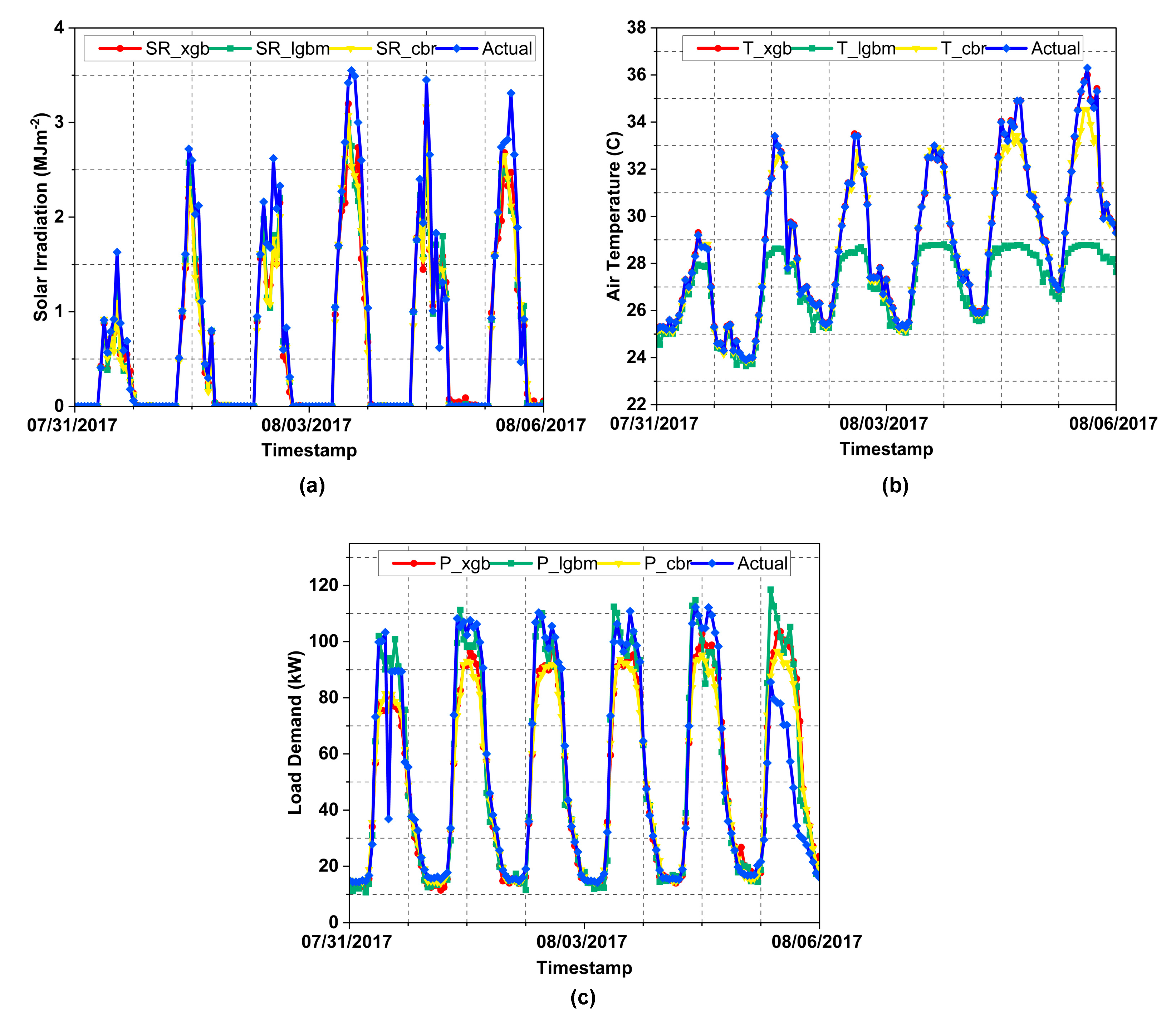
4.1. Performance Assessment of Ensemble Methods for Forecasting of Solar Radiation, Air Temperature and Load Demand

In this study, three different ensemble ML algorithms, XGB, LGBM and CBR, were evaluated for their accuracy in forecasting the input variables of our system, specifically SR, AT and LD at the target location. The hyperparameters of the models were finetuned and the optimized values for these parameters for each model are presented in

Table A2. Optimized hyperparameters of ML model for three different learning tasks.

ML Models	Hyperparameters	SR Prediction Task	AT Prediction Task	LD Prediction Task
XGB	Colsample by tree	0.06	0.96	0.33
	Gamma	0.85	0.23	0.46
	Learning rate	0.03	0.02	0.10
	Max. depth	8.00	2.00	2.00
	Min. child weight	7.00	9.00	8.00
	Estimators (102)	13.00	80.00	90.00
	Objective function	Squared error	Absolute error	Absolute error
	Alpha	0.99	0.78	0.11
	Lambda	0.50	0.78	0.45
	Subsample	0.44	0.83	0.10
LGBM	Bagging fraction	0.60	0.50	0.40
	Bagging frequency (102)	1.00	4.00	5.00
	Boosting	Dart	Dart	Gbdt
	Feature fraction	0.80	0.70	0.37
	Learning rate	0.10	0.10	0.14
	Max. depth	10.00	40.00	10.00
	Min. data in leaf	15.00	50.00	20.00
	Estimators (102)	50.00	10.00	70.00
	Number of leaves	45.00	60.00	20.00
	Objective function	Mean absolute error	Mean absolute error	-
CBR	Bagging temperature	0.16	0.06	0.95
	Border count (102)	1.90	2.44	1.48
	Depth	10.00	4.00	6.00
	Iterations (102)	10.00	7.00	3.00
	L2 leaf	7.28	9.87	8.12
	Learning rate	0.07	0.38	0.04
	Od type	IncToDec	Iter	IncToDec
	Od wait	15.00	22.00	28.00
	Random strength	3.57	1.53	51.50

in Appendix A. A graphical comparison of the forecasted and observed values for each hypertuned model for a one-week period is presented in Figure 8.

The overall investigation of these hourly forecasts reveals that the LGBM model outperforms the other models for the data with no cyclic trends, as reflected by the results for the SR and LD prediction tasks in Figure 8a,c, respectively. On the other hand, the other two models were found to capture the increasing trends in the cyclic patterns more accurately, as reflected by the results in Figure 8b and Table 6 for the air temperature forecast. The air temperature data showed an increasing and decreasing trend in the values over the 24 h period, such that the peak temperature was achieved slightly later than noon, followed by a steady decline in temperature until it reached a typical value of 25 °C at the end of the day. The repetition of this pattern is evident throughout the week; however, the intensity of the temperature varies, as does the duration in reaching the peak temperature over the whole week. For instance, for the first day, the peak temperature of 29.2 °C was reached at 14:00 h, while the peak temperature of the fourth day was recorded to be 33 °C at 16:00 h. The MAE and R2 metrics were calculated for each model as quantitative measures of the prediction performance and are presented in

Table 7. Performance evaluation of ML models based on statistical metrics.

Regression Task	ML Algorithm	Performance Metric
		MAE	R2
SR prediction	XGB	0.1573	0.9139
	LGBM	0.0945	0.9433
	CBR	0.0985	0.9422
AT prediction	XGB	0.0241	0.9999
	LGBM	0.2967	0.9956
	CBR	0.0637	0.9998
LD prediction	XGB	11.4073	0.7366
	LGBM	10.8954	0.6996
	CBR	11.4797	0.7280

SR: solar radiation, AT: air temperature, LD: load demand, XGB: extreme gradient boosting, LGBM: light gradient boosting machine, CBR: cat boost regressor, MAE: mean absolute error, R2: coefficient of determination.

. The results indicate that, overall, the LD prediction models’ performance is poor relative to the SR and AT models, which is in line with the expected outcome, as the training data for LD prediction were ten times less than the data used to train the other models.

The prediction performance of machine learning algorithms usually depends on the type of algorithm, the nature of the data, the amount of data and the hyperparameters of the algorithm. In this study, all implemented ML algorithms are built on the boosting gradient machine algorithm and are applied on weather and load demand time series data. Additionally, almost all hyperparameters of these algorithms are optimized. Based on the provided results in Table 7, CBR seems to be the worst performer compared to XGB and LGBM for all three prediction tasks; it is commonly known for its application in classification tasks. This is because the encoding of categorical features in CBR is based on the output columns, considering the weightage of the output column during training or encoding. This feature makes cat boost more accurate on categorical datasets. However, this encoding method may not be optimal for regression tasks such as the one in our case, where the performance of CBR was the worst among the three algorithms. The XGB and LGBM models showed higher prediction errors for the SR and AT prediction tasks. This might be because of the lack of informative features in the training data, as these models were already optimized and the amount of training data was also adequate.

4.2. Comparative Performance Evaluation of Optimization Algorithms

The performance evaluation of an optimization algorithm is conducted by investigating its accuracy, execution time and convergence characteristics. The algorithm’s accuracy can be analyzed by comparing the obtained objective function values, while the convergence performance is evaluated by the number of iterations required to reach the global optimum. In this study, nine different optimization algorithms were employed to minimize the TNPC of the HRES, under the constraint of five values of DRPSP_max.

Table 8. Summary of sizing results obtained by optimization algorithms for 0% DRPSP_max.

DRPSPmax	Optimization Algorithm	Average Time (s)	Time Standard Deviation	Average TNPC (Million $)	TNPC Standard Deviation
0%	AGWOCS	219.1	4.1	3.262	0.000
	CPSOGSA	219.9	5.4	3.262	0.000
	dFDBMRFO	6.5	0.1	3.262	0.000
	EHOTOPSIS	219.4	5.1	3.546	0.148
	FDBSFS	876.8	18.7	3.262	0.000
	FDBTLABC	6.5	0.2	3.262	0.000
	HFPSO	222.4	5.9	3.285	0.036
	HPSOBOA	346.8	8.3	3.591	0.173
	HSSOGSA	219.3	3.9	3.262	0.000

TNPC: total net present cost.

,

Table 9. Summary of sizing results obtained by optimization algorithms for 1.3% DRPSP_max.

DRPSPmax	Optimization Algorithm	Average Time (s)	Time Standard Deviation	Average TNPC (Million $)	TNPC Standard Deviation
1.3%	AGWOCS	216.3	4.2	1.465	0.241
	CPSOGSA	216.8	5.0	1.461	0.000
	dFDBMRFO	6.3	0.2	1.461	0.641
	EHOTOPSIS	215.5	7.0	2.723	0.000
	FDBSFS	862.5	15.5	1.461	0.641
	FDBTLABC	6.3	0.1	1.461	0.460
	HFPSO	218.3	6.2	1.571	0.000
	HPSOBOA	335.0	6.9	1.676	0.217
	HSSOGSA	216.8	4.8	1.461	0.209

,

Table 10. Summary of sizing results obtained by optimization algorithms for 2% DRPSP_max.

DRPSPmax	Optimization Algorithm	Average Time (s)	Time Standard Deviation	Average TNPC (Million $)	TNPC Standard Deviation
2%	AGWOCS	219.5	4.7	1.315	0.028
	CPSOGSA	221.4	6.1	1.313	0.000
	dFDBMRFO	6.4	0.1	1.313	0.000
	EHOTOPSIS	220.6	5.4	2.385	0.000
	FDBSFS	881.3	23.2	1.313	0.075
	FDBTLABC	6.4	0.2	1.313	0.032
	HFPSO	221.1	4.5	1.374	0.025
	HPSOBOA	342.3	7.9	1.338	0.163
	HSSOGSA	219.4	5.0	1.371	0.031

and

Table 11. Summary of sizing results obtained by optimization algorithms for 5% DRPSP_max.

DRPSPmax	Optimization Algorithm	Average Time (s)	Time Standard Deviation	Average TNPC (Million $)	TNPC Standard Deviation
5%	AGWOCS	218.3	5.1	1.103	0.000
	CPSOGSA	217.4	3.8	1.103	0.000
	dFDBMRFO	6.3	0.2	1.103	0.000
	EHOTOPSIS	217.8	5.9	2.720	0.014
	FDBSFS	864.5	16.6	1.105	0.115
	FDBTLABC	6.3	0.2	1.126	0.000
	HFPSO	221.5	6.0	1.103	0.000
	HPSOBOA	336.4	8.6	1.103	0.000
	HSSOGSA	217.1	4.4	1.103	0.000

present the optimum values of the averaged TNPC obtained by different algorithms and their average execution times for different values of DRPSP_max. These algorithms are stochastic as the optimized result might change with multiple runs. To ensure the consistency of the results, the optimization procedure was repeated for 25 runs and the results were averaged and for each independent run; the algorithm ran for a maximum of 100 iterations. The computational time required by an optimization algorithm is an essential factor that plays a critical role when assessing the algorithm’s performance. The amount of data that the algorithm has to process is one of the main contributors to this time value. The performance of these optimization algorithms in terms of the convergence and execution time required for HRES capacity optimization while satisfying all constraints is shown in Figure 9. The results in Figure 9a indicate that the AGWOCS algorithm outperforms the others, reaching the optimal solution within 30 iterations.

Figure 9b illustrates that the novel fitness–distance balance selection strategy resulted in the fastest execution time, with an average of 6.38 s, except for the FDBSFS algorithm, which was the most computationally expensive, with an average execution time of 871.26 s. All other algorithms, excluding HPSOBOA, reached the optimal solution within a maximum of 218.98 s, while HPSOBOA required 340.13 s. The TNPC averages of the optimally sized HRES with varying values of DRPSP_max are presented in Figure 10. It can be seen that for all the algorithms, the TNPC decreases with the decreasing DRPSP_max value. The overall result indicates that six out of the nine algorithms (AGWOCS, CPSOGSA, dFDBMRFO, HFPSO, HPSOBOA and HSSOGSA) optimize the cost of the HRES to a minimum average value of USD 1.103 million. Further analysis revealed that the EHOTOPSIS algorithm results in the highest value of USD 2.72 million as the optimal TNPC. As expected, increasing the DRPSP_max value from 0 to 5% leads to a cost saving of approximately USD 2.159 million, which can be found by subtracting the minimum cost obtained for 0% DRPSP_max (USD 3.262 million) and 5% DRPSP_max (USD 1.103 million). Conversely, restricting the HRES to supply power 100% of the time (DRPSP_max = 0%) leads to additional costs.

The dFDBMRFO and FDBTLABC hybrid algorithms demonstrated superior performance in terms of execution time, whereas the lowest TNPC was obtained by the majority of the optimization algorithms. The robustness of these algorithms is also reflected in the standard deviation values calculated based on the average time and objective function value achieved by the algorithms. In the optimization of the HRES capacity and operation, it is essential to strike a balance between the computational resources required and the cost savings achieved. It should be noted that the execution time of the optimization algorithm in capacity optimization is a one-time investment and should be weighed against the economic benefits obtained. In this study, most of the algorithms successfully reached the optimal solution of the lowest TNPC (USD 1.103 million) but the computational effort required by each algorithm was different. Among all algorithms that reached an optimal solution, the dFDBMRFO algorithm was the fastest, with an average computation time of 6.30 s. CPSOGSA was selected as the optimal choice for HRES capacity optimization due to its stability of results; although its computational time requirement was high, as capacity optimization is not a dynamic optimization problem, it was acceptable.

All the implemented algorithms were further compared based on their convergence performance and the reproducibility of their results. The data provided in

Table 12. Comparison of performance of implemented optimization algorithms based on their convergence characteristics, computational requirements and results’ reproducibility.

Algorithm	Iterations to Convergence	Average Computational Time	Results Stability (Avg. Standard Deviation)	Lowest Cost Achieved (Million $)
AGWOCS	31	218.290	0.067	1.103
CPSOGSA	37	218.850	0.000	1.103
dFDBMRFO	100	6.370	0.160	1.103
EHOTOPSIS	100	218.310	0.003	2.720
FDBSFS	88	871.260	0.207	1.105
FDBTLABC	45	6.380	0.123	1.126
HFPSO	23	220.820	0.015	1.103
HPSOBOA	6	340.130	0.130	1.103
HSSOGSA	30	218.130	0.060	1.103

reveal that some algorithms require fewer iterations to reach the lowest TNPC, such as HFPSO and HPSOBOA, which only need 23 and 6 iterations, respectively. This suggests that these algorithms are more efficient in finding the optimal solution compared to other algorithms. A possible reason is that the update of the search agents’ positions in HFPSO is not influenced by previous positions, especially during the local search, and thus avoids entrapment in local minima. As for the HPSOBOA, this faster convergence rate is due to the novel cubic 1D initialization of search agents, which distributes the search agents without any biasing evenly over the entire search domain. However, their average computational times are relatively high compared to other algorithms, with HPSOBOA having the highest computational time of 340.130 s. This indicates that while these algorithms can quickly find the optimal solution, they may not be practical for real-world applications that require fast results, such as the dynamic operation optimization of HRES. On the other hand, dFDBMRFO has the lowest average computational time of 6.370 s, but it requires 100 iterations to reach the lowest TNPC. However, the convergence characteristic showed continuous convergence even when it reached the maximum iterations. This indicates that this algorithm is computationally efficient due to the incorporation of a dynamically varying constant based on the convergence result in each iteration, but it may require more iterations to find the optimal solution compared to other algorithms. In terms of results’ stability, CPSOGSA has an average standard deviation of 0.000, indicating that its results are the most stable, which suggests that CPSOGSA is a reliable algorithm that can consistently produce optimal solutions, which is essential for decision making and reflects that the algorithm effectively searches the whole search space for the global optima because of the refined local search with consideration of the mass interaction concept of search particles introduced by GSA. However, some algorithms have relatively higher standard deviations, such as FDBSFS with 0.207, dFDBMRFO with 0.160 and FDBTLABC with 0.123. This means that these algorithms are relatively less reliable as their results may vary more, indicating that the FDB selection methods are more sensitive to random perturbation. Finally, all algorithms reached the same lowest cost value of USD 1.103 million, except EHOTOPSIS, which reaches USD 2.720 million. This suggests that all algorithms, except EHOTOPSIS, are capable of finding the optimal solution. However, EHOTOPSIS’s suboptimal performance may be due to its entrapment in local minima and it may require finetuning of its parameters.

4.3. Optimal Sizing of HRES

This study aimed to find the optimal size of a HRES that minimizes the TNPC while satisfying all the constraints, such as the required system reliability (DRPSP), zero net energy balance, bounds on decision variables, SOC limit and the minimum required REF. Using 15 years of ML-forecasted data for renewable resources and load demands, the optimization results of the average TNPC as a function of the obtained DRPSP value for REF ranging from 10 to 60% are as presented in Figure 11. Although the minimum allowed REF was set to 30%, a sensitivity analysis was conducted to explore the potential of renewable energy at the target location for comparison. The analysis confirmed the negative correlation between TNPC and DRPSP and showed that increasing the allowed REF reduced the DRPSP but increased the TNPC. For instance, when the system size is optimized under the constraint of 0–5% DRPSP_max, the increase in REF from 10 to 60% leads to a reduction in the obtained DRPSP value from 2.3 to 0% but results in a maximum increase in the average TNPC from USD 0.672 million to USD 3.732 million. In addition, fixing the required REF at 30%, as chosen for the proposed system, the increase in system cost when setting up a highly reliable HRES (DRPSP: 0%) compared to that of allowing for a certain level of interruption in the power supply (DRPSP: 0.023%) is USD 2.160 million. Through the optimization process, an optimal solution was identified for the proposed HRES, as indicated by the red star in Figure 11. The selected solution is neither the cheapest nor the most reliable option, but rather provides a balance between the cost (USD 1.46 million) and an acceptable level of interruption in the power supply (DRPSP: 0.013%). It is important to note that this level of DRPSP is suitable for the target location, as the proposed HRES is connected to the main electric grid and thus can serve as a backup power source on days when the HRES power supply is inadequate. However, for isolated communities that rely solely on renewable energy, minimizing the DRPSP is of greater concern than the non-recurrent investment cost of TNPC, since a non-zero DRPSP means no electricity. The detailed results of the HRES capacity optimization process using various algorithms are presented in

Table 13. HRES capacity optimized by various algorithms for 0% DRPSP_max at 30% minimum allowed REF.

DRPSPmax	Optimization Algorithm	NPV	NBAT	NINV	REF	DRPSP	CO2 (ton/MWh)	TNPC (106 $)
0%	AGWOCS	303	115	31	0.301	0.000	1757	3.262
	CPSOGSA	303	115	31	0.301	0.000	1757	3.262
	dFDBMRFO	303	115	31	0.301	0.000	1757	3.262
	EHOTOPSIS	329	127	34	0.332	0.000	1703	3.546
	FDBSFS	303	115	31	0.301	0.000	1757	3.262
	FDBTLABC	303	115	31	0.301	0.000	1757	3.262
	HFPSO	305	116	31	0.303	0.000	1753	3.285
	HPSOBOA	304	132	35	0.302	0.000	1755	3.591
	HSSOGSA	303	115	31	0.301	0.000	1757	3.262

TNPC: total net present cost, REF: renewable energy fraction, DRPSP: deficiency of power supply probability.

,

Table 14. HRES capacity optimized by various algorithms for 1.3% DRPSP_max at 30% minimum allowed REF.

DRPSPmax	Optimization Algorithm	NPV	NBAT	NINV	REF	DRPSP	CO2 (ton/MWh)	TNPC (×106 $)
1.3%	AGWOCS	307	21	10	0.303	0.013	1755	1.465
	CPSOGSA	305	21	10	0.301	0.013	1759	1.461
	dFDBMRFO	305	21	10	0.301	0.013	1759	1.461
	EHOTOPSIS	672	48	22	0.729	0.004	1238	2.723
	FDBSFS	305	21	10	0.301	0.013	1759	1.461
	FDBTLABC	305	21	10	0.301	0.013	1759	1.461
	HFPSO	321	25	11	0.320	0.011	1726	1.571
	HPSOBOA	325	30	12	0.325	0.010	1715	1.676
	HSSOGSA	305	21	10	0.301	0.013	1759	1.461

,

Table 15. HRES capacity optimized by various algorithms for 2% DRPSP_max at 30% minimum allowed REF.

DRPSPmax	Optimization Algorithm	NPV	NBAT	NINV	REF	DRPSP	CO2 (ton/MWh)	TNPC (×106 $)
2%	AGWOCS	309	13	8	0.302	0.020	1759	1.315
	CPSOGSA	308	13	8	0.301	0.020	1761	1.313
	dFDBMRFO	308	13	8	0.301	0.020	1761	1.313
	EHOTOPSIS	952	4	17	0.901	0.018	1358	2.385
	FDBSFS	308	13	8	0.301	0.020	1761	1.313
	FDBTLABC	308	13	8	0.301	0.020	1761	1.313
	HFPSO	458	1	8	0.430	0.020	1616	1.374
	HPSOBOA	330	12	8	0.323	0.020	1726	1.338
	HSSOGSA	446	2	8	0.421	0.020	1621	1.371

and

Table 16. HRES capacity optimized by various algorithms for 5% DRPSP_max at 30% minimum allowed REF.

DRPSPmax	Optimization Algorithm	NPV	NBAT	NINV	REF	DRPSP	CO2 (ton/MWh)	TNPC (×106 $)
5%	AGWOCS	320	1	6	0.300	0.021	1771	1.103
	CPSOGSA	320	1	6	0.300	0.021	1771	1.103
	dFDBMRFO	320	1	6	0.300	0.021	1771	1.103
	EHOTOPSIS	949	21	21	0.942	0.010	1250	2.72
	FDBSFS	321	1	6	0.301	0.021	1770	1.105
	FDBTLABC	322	2	6	0.304	0.021	1765	1.126
	HFPSO	320	1	6	0.300	0.021	1771	1.103
	HPSOBOA	320	1	6	0.300	0.021	1771	1.103
	HSSOGSA	320	1	6	0.300	0.021	1771	1.103

, including the optimal numbers of PV panels, batteries and power inverters, and the attained REF, DRPSP, CO₂ emissions and TNPC.

The results indicate that all the algorithms except EHOTOPSIS, HFPSO and HPSOBOA were able to reach the optimal lowest-cost solution for four different cases of DRPSP_max. It was observed that, in general, optimization algorithms HFPSO and HPSOBOA performed better, except at a DRPSP_max of 2%, than EHOTOPSIS, which had the worst performance. The optimal solutions reveal that increasing the DRPSPmax from 0 to 5% increases the PV panels by 17 units, while the numbers of batteries and power inverters are reduced by 114 and 25 units, respectively. As the constraint on the HRES in maintaining a continuous power supply is relaxed, the optimization process leads to a significant decrease in battery energy storage units. These energy storage units act as backup power supply units in the event that production from the RE units becomes insufficient to meet the load demand, thus satisfying the strict reliability of the power supply. The number of power inverters (NINV) is not treated as a decision variable in the optimization process but is calculated based on the maximum power flow through optimally sized PV power generators and battery packs. Similarly, CO₂ emissions are calculated based on energy purchased from the main grid, as the only non-renewable energy source.

The variation in the values of the objective functions, including TNPC as a function of the decision variables ($N_{PV}, N_{BAT}$), is illustrated in Figure 12. The visual analysis reveals that the different clusters formed are associated with the attained optimal values of the average TNPC. In contrast, variation within the clusters reflects the optimization performance of different algorithms. The optimal HRES size includes 305 PV panels, 21 batteries and 10 power inverters and was determined by selecting a solution that provided a reasonable balance between cost and power supply reliability. The system costs about USD 1.46 million, releases 1759 ton/MWh CO₂ emissions and is unable to satisfy the LD using renewable sources over the whole simulation period of 15 years, for about 73 days, corresponding to a DRPSP of 1.3%. The values of the input parameters in this optimization analysis are presented in

Table 17. Selected values of input parameters for optimal HRES.

Inflation Rate	Interest Rate	Grid Purchase Unit Price	Grid Sellback Unit Price	PV Efficiency	Battery DOD
5%	3.26%	0.07 $/kWh	0.098 $/kWh	20.1%	80%

DOD: depth of discharge.

.

4.4. Operation Simulation Analysis of Optimal HRES

The operation of the optimally sized HRES system was simulated and the power balance analysis over a typical 24 h period for four different seasons is presented in Figure 13. The positive value of the battery power indicates the charging of the battery ESS with a corresponding increase in battery SOC, while a negative value means battery ESS discharging reflected by a decrease in battery SOC. The power balance analysis was performed under the energy management strategy adopted to optimize the HRES capacity, where the excess electricity generated is sold to the grid only after the battery ESS with a set capacity is fully charged, ensuring that it is utilized to its fullest potential. This approach of selling excess energy to the grid, rather than storing it in the battery ESS, which requires the expansion of the existing capacity of the battery storage system, is more economical and helps to minimize the TNPC of the HRES. The overall analysis reveals that there is abundant renewable power production during the daytime for all seasons, with the HRES operating at its full potential in the spring due to the abundant sunlight and moderate LD. On a typical day in the spring and fall seasons, the HRES production starts with a minimum of about 2 kW at 6:00 and reaches a peak of nearly 65 kW by noon. In the summer, the peak production is around 85 kW, while, in the winter, the lowest amount of power of about 1 kW is generated. The LD for nighttime is fulfilled by purchasing from the electric grid for all seasons, because the optimal HRES includes the minimal number of batteries, resulting in better financial prospects over the long-term period.

4.5. Comparison of Sizing Results against 15-Year and 1-Year Scenarios

The primary objective of the current study was to validate the hypothesis that HRES capacity optimization using ML-predicted inputs over 15 years results in a more realistic HRES capacity, compared to the traditional optimization strategy where the input data for the first year are extended over the next 15 years. A comparative study was performed under the following two scenarios: the first was based on predicted input data for 15 years, while the second was based on repeating one year’s input data for 15 years. It is worth noting that while the optimal system obtained through the first scenario might not necessarily be low-cost, it would be more representative of the actual conditions with an increasing frequency of extreme weather variations. The detailed optimization results of the first scenario are presented in Table 13, Table 14, Table 15 and Table 16, while the results of the second scenario are presented in

Table 18. HRES capacity optimized by various algorithms for 0% DRPSP_max at 30% minimum allowed REF in second scenario.

DRPSPmax	Optimization Algorithm	NPV	NBAT	NINV	REF	DRPSP	CO2 (ton/MWh)	TNPC (×106 $)
0%	AGWOCS	265	114	30	0.301	0.000	1731	3.179
	CPSOGSA	264	114	30	0.300	0.000	1733	3.177
	dFDBMRFO	264	114	30	0.300	0.000	1733	3.177
	EHOTOPSIS	697	125	40	0.970	0.000	817	4.262
	FDBSFS	264	114	30	0.300	0.000	1733	3.177
	FDBTLABC	264	114	30	0.300	0.000	1733	3.177
	HFPSO	293	114	31	0.340	0.000	1661	3.235
	HPSOBOA	310	128	34	0.364	0.000	1619	3.538
	HSSOGSA	264	114	30	0.300	0.000	1733	3.177

TNPC: total net present cost, REF: renewable energy fraction, DRPSP: deficiency of power supply probability.

,

Table 19. HRES capacity optimized by various algorithms for 1.3% DRPSP_max at 30% minimum allowed REF in second scenario.

DRPSPmax	Optimization Algorithm	NPV	NBAT	NINV	REF	DRPSP	CO2 (ton/MWh)	TNPC (×106 $)
1.3%	AGWOCS	266	21	9	0.302	0.013	1730	1.395
	CPSOGSA	265	21	9	0.301	0.013	1732	1.393
	dFDBMRFO	265	21	9	0.301	0.013	1732	1.393
	EHOTOPSIS	460	28	14	0.554	0.008	1367	1.909
	FDBSFS	265	21	9	0.301	0.013	1732	1.393
	FDBTLABC	265	21	9	0.301	0.013	1732	1.393
	HFPSO	303	25	11	0.351	0.011	1642	1.546
	HPSOBOA	265	32	12	0.301	0.009	1731	1.604
	HSSOGSA	265	21	9	0.301	0.013	1732	1.393

,

Table 20. HRES capacity optimized by various algorithms for 2% DRPSP_max at 30% minimum allowed REF in second scenario.

DRPSPmax	Optimization Algorithm	NPV	NBAT	NINV	REF	DRPSP	CO2 (ton/MWh)	TNPC (×106 $)
2%	AGWOCS	351	2	6	0.388	0.020	1607	1.191
	CPSOGSA	351	2	6	0.388	0.020	1607	1.191
	dFDBMRFO	351	2	6	0.388	0.020	1607	1.191
	EHOTOPSIS	289	38	14	0.334	0.007	1671	1.768
	FDBSFS	351	2	6	0.388	0.020	1607	1.191
	FDBTLABC	351	2	6	0.388	0.020	1607	1.191
	HFPSO	352	1	6	0.387	0.020	1610	1.173
	HPSOBOA	337	4	7	0.376	0.020	1620	1.203
	HSSOGSA	351	2	6	0.388	0.020	1607	1.191

and

Table 21. HRES capacity optimized by various algorithms for 5% DRPSP_max at 30% minimum allowed REF by second scenario.

DRPSPmax	Optimization Algorithm	NPV	NBAT	NINV	REF	DRPSP	CO2 (ton/MWh)	TNPC (×106 $)
5%	AGWOCS	273	1	5	0.300	0.021	1739	1.022
	CPSOGSA	273	1	5	0.300	0.021	1739	1.022
	dFDBMRFO	273	1	5	0.300	0.021	1739	1.022
	EHOTOPSIS	755	33	20	0.908	0.005	1096	2.560
	FDBSFS	273	1	5	0.300	0.021	1739	1.022
	FDBTLABC	273	1	5	0.300	0.021	1739	1.022
	HFPSO	274	1	5	0.301	0.021	1737	1.024
	HPSOBOA	282	2	5	0.312	0.021	1719	1.059
	HSSOGSA	273	1	5	0.300	0.021	1739	1.022

.

The results of the comparative analysis of the two optimization scenarios are summarized in

Table 22. Summary of HRES capacity optimization results for two studied scenarios.

Scenario	Simulation Duration	Simulated System	Obtained DRPSP	Obtained REF	CO2 Emissions	Grid Power Purchased	Grid Power Sold	Battery Utility
First Based on 15-year data	15 years	NPV: 305, NBAT: 21, NPI: 10	0.0128	30%	1759 tons/MWh	429 MW	15929 kW	11%
Second Based on repeat of 1-year data	15 years	NPV: 265, NBAT: 21, NPI: 9	0.0134	25%	1732 tons/MWh	448 MW	2224 kW	8%

. The optimal HRES design for the second scenario comprised 265 PV panels, 21 batteries and 9 power Inverters. The system cost was estimated at USD 1.39 million and it produced 1732 ton/MWh CO₂ emissions, and the probability of a deficient power supply was estimated at a maximum of 73 days. The comparative results demonstrated that the optimal capacity of the HRES obtained in the second scenario was relatively smaller. This discrepancy can be attributed to the limited representation of the RE resources and LD in the second scenario, which relied on repeated patterns over a single year of data. In contrast, the first scenario utilized accurate ML predictions of the RE resources and LD over the entire project lifespan, providing a more realistic representation of the actual conditions. As a result of the lower HRES optimum capacity, the TNPC obtained in the second scenario for the optimum HRES was USD 68,000 less than that of the first scenario, with similar power supply reliability and lower CO₂ emissions.

The analysis of these results highlights the difference in the HRES capacities obtained in the two scenarios. While the HRES capacity obtained in the second scenario appears to be more economical and provides a similar level of renewable power supply reliability, its performance falls short of satisfying the set constraints (REF: 25% < 30%, DRPSP: 0.0134 > 0.0130) when both systems are simulated for their lifetimes, as indicated by the results in Table 10. This system, as opposed to the system obtained in the first scenario, purchased 0.2 MW more electricity from the main electric grid, sold 14 kW less energy to the main grid, released 27 ton/MWh more CO₂ emissions and experienced a 3-day-longer power loss period during its operation. Additionally, the utilization of the battery ESS was assessed by operating the optimized system for both scenarios based on actual 15-year data and results showed that the system obtained from the second scenario resulted in a 3% reduction in ESS usage, leading to a higher self-discharge rate, contributing to the reduced ESS life.

5. Conclusions

The integration of HRES with the main grid has become the preferred strategy to satisfy the energy requirements of urban areas by providing a reasonable mix of renewable energy with non-renewable energy at an affordable cost. However, the economically and technically viable grid integration of such systems is hindered by the intermittent and unpredictable nature of renewable energy production. One way to mitigate these drawbacks is by using AI-based data-driven forecasts while optimizing the size of HRES. However, nearly all HRES sizing studies in the literature utilize only 1 year’s data for the LD and RE resources to decide on the optimal system size. These results are then projected into the future based on the inaccurate assumption that the LD and the weather patterns will repeat themselves over the whole lifespan of the HRES. In this study, a grid-connected HRES for a commercial building in Gwangju, South Korea, is optimally sized based on the deep learning data forecasts of the load demand and solar radiation for 15 years. The results of ten different optimization algorithms were compared to find the optimal HRES that would incur the smallest cost while satisfying the constraints of the power balance, DRPSP and REF.

The new data-driven framework integrating AI and hybrid metaheuristics for HRES capacity optimization was implemented by simulating two scenarios, such that ML-based forecasted data in the form of two different datasets were evaluated for the HRES’ optimal sizing. The first dataset contained only a single year of forecasted data, which were repeated 15 times to obtain a whole dataset under the unrealistic assumption of repeated weather patterns. On the other hand, the second dataset contained input data (SR, AT and LD) forecasted over a 15-year period. In the first scenario, the entire set of 15-year input data forecasted by ML was fed as input into the optimization solver in MATLAB to optimize the capacity of the HRES for a 15-year project life. In contrast, the second scenario utilized the repeated dataset as input for HRES capacity optimization. Lastly, a sensitivity analysis based on the interest rate, inflation rate, grid-related costs and PV panel efficiency was conducted on the proposed HRES. The following conclusions are drawn from our study:

• The novel data-driven HRES capacity optimization framework considered as the first scenario proposed in this study was found to result in a different optimal HRES size compared to the second scenario. The difference is reflected by the obtained values of the HRES constraints at the end of optimization, including REF and DRPSP, with values of 30% and 0.0128, respectively, for the first scenario. On the other hand, the system obtained through the second scenario resulted in a 25% REF, which was 5% less than the set limit, as well as a DRPSP of 0.0134, which was larger than the set limit of 0.0130. In addition, the first system also purchased 4% less and sold 86% more power to the main electrical grid, respectively, with 4% less CO₂ emissions.
• The comparison of results found that when optimizing the HRES capacity, it is better to utilize simulation input data spanning the whole life of the targeted HRES. However, further investigation is required to confirm whether the proposed data-driven approach provides more realistic HRES sizing results than the conventional yearly-based simulations.
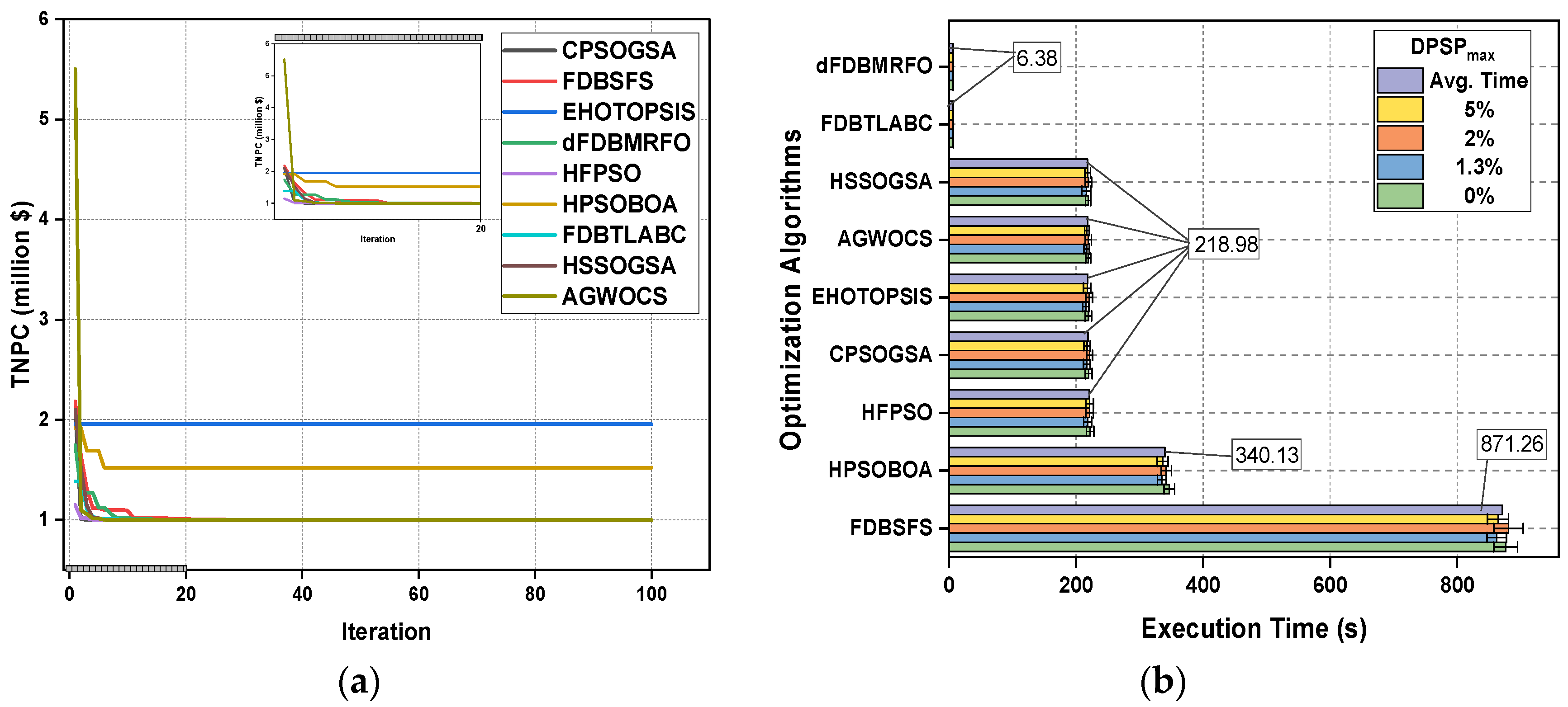
• The comparative performance analysis of the optimization algorithms showed that the dFDBMRFO algorithm is the best in terms of computational time, while the CPSOGSA algorithm finds the lowest HRES cost within a reasonable time.
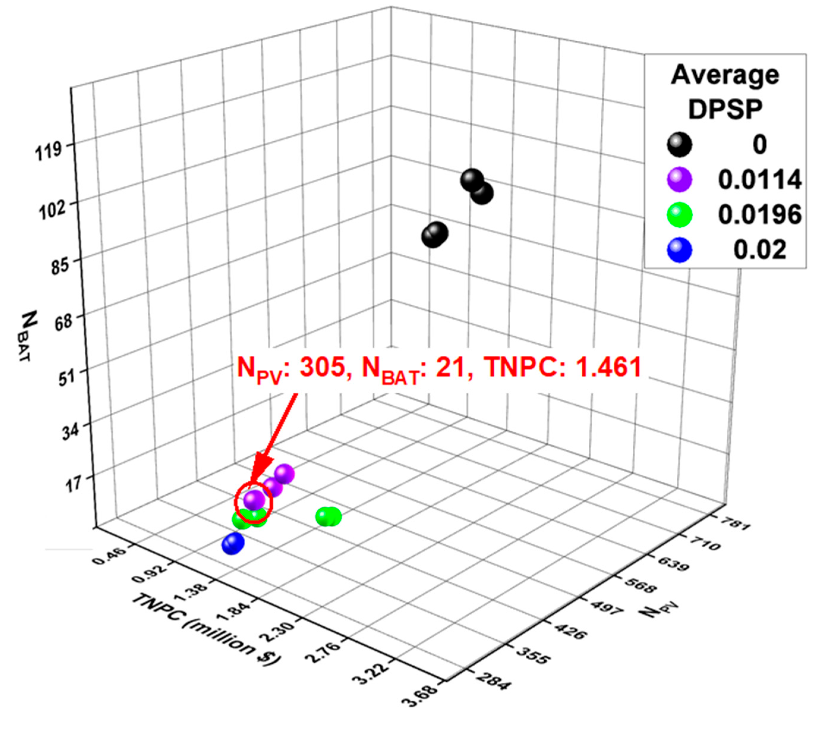
• The optimal HRES, under the constraint of DRPSPmax of 1.3%, consists of 305 PV panels, 21 batteries and 10 power inverters, with a TNPC of USD 1.46 million, including grid interaction costs. The proposed system satisfies all the constraints such that the values of DRPSP and REF obtained are 0.013 and 0.3, respectively, both of which satisfy the specified limits.
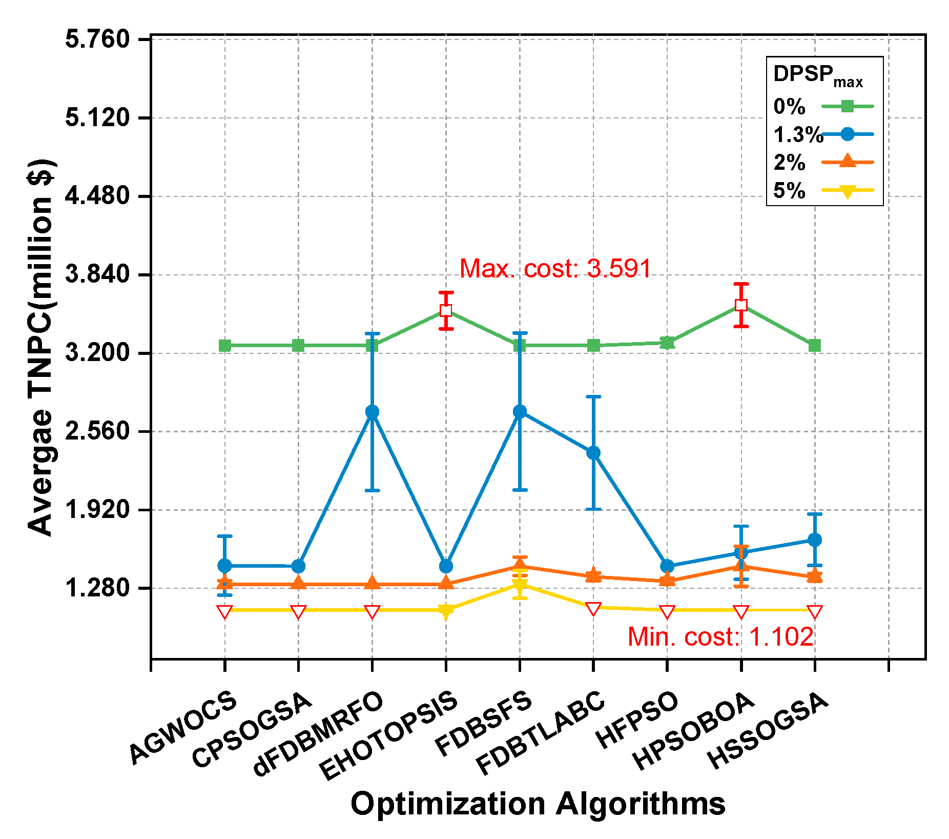
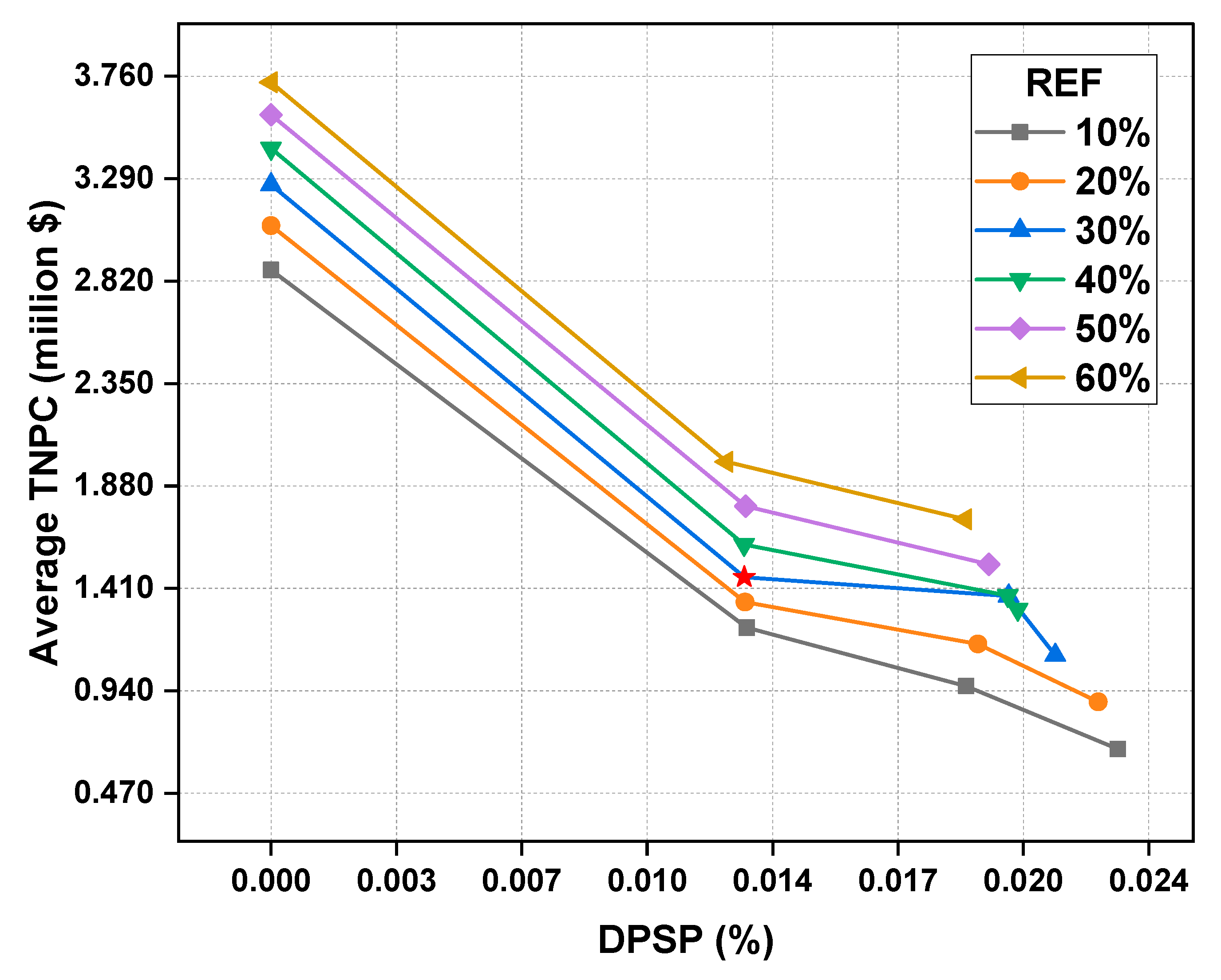
• The comparison of various proposed HRES based on the environmental impact and power supply reliability revealed that minimizing the environmental impact increases the HRES capacity and corresponding TNPC by as much as 25%. The TNPC value almost triples for HRES with zero probability of a deficient power supply over the project lifespan.

References

1. United Nations Department of Economic and Social Affairs, Population Division. World Population Prospects 2022: Summary of Results; United Nations: New York, NY, USA, 2022; p. 52. [Google Scholar]
2. International Energy Agency. World Energy Outlook; IEA: Paris, France, 2021; p. 386. [Google Scholar]
3. Caetano, N.S.; Mata, T.M.; Martins, A.A.; Felgueiras, M.C. New Trends in Energy Production and Utilization. Energy Procedia 2017, 107, 7–14. [Google Scholar] [CrossRef]
4. Capuano, D.L. International Energy Outlook 2018 (IEO2018); U.S. Energy Information Administration: Washington, DC, USA, 2018; p. 21.
5. Clarke, B.; Otto, F.; Stuart-Smith, R.; Harrington, L. Extreme Weather Impacts of Climate Change: An Attribution Perspective. Environ. Res. Clim. 2022, 1, 012001. [Google Scholar] [CrossRef]
6. Konisky, D.M.; Hughes, L.; Kaylor, C.H. Extreme Weather Events and Climate Change Concern. Clim. Chang. 2016, 134, 533–547. [Google Scholar] [CrossRef]
7. International Energy Agency. Net Zero by 2050—A Roadmap for the Global Energy Sector; IEA: Paris, France, 2021; p. 224. [Google Scholar]
8. Stram, B.N. Key Challenges to Expanding Renewable Energy. Energy Policy 2016, 96, 728–734. [Google Scholar] [CrossRef]
9. Ciupageanu, D.-A.; Barelli, L.; Lazaroiu, G. Real-Time Stochastic Power Management Strategies in Hybrid Renewable Energy Systems: A Review of Key Applications and Perspectives. Electr. Power Syst. Res. 2020, 187, 106497. [Google Scholar] [CrossRef]
10. Sinsel, S.R.; Riemke, R.L.; Hoffmann, V.H. Challenges and Solution Technologies for the Integration of Variable Renewable Energy Sources—A Review. Renew. Energy 2020, 145, 2271–2285. [Google Scholar] [CrossRef]
11. Adnan, M.; Tariq, M.; Zhou, Z.; Poor, H.V. Load Flow Balancing and Transient Stability Analysis in Renewable Integrated Power Grids. Int. J. Electr. Power Energy Syst. 2019, 104, 744–771. [Google Scholar] [CrossRef]
12. IRENA; ILO. Renewable Energy and Jobs Annual Review; International Renewable Energy Agency International Labour Organization: Abu Dhabi, Geneva, 2021; ISBN 978-92-9260-364-9. [Google Scholar]
13. Alberizzi, J.C.; Frigola, J.M.; Rossi, M.; Renzi, M. Optimal Sizing of a Hybrid Renewable Energy System: Importance of Data Selection with Highly Variable Renewable Energy Sources. Energy Convers. Manag. 2020, 223, 113303. [Google Scholar] [CrossRef]
14. Memon, S.A.; Patel, R.N. An Overview of Optimization Techniques Used for Sizing of Hybrid Renewable Energy Systems. Renew. Energy Focus 2021, 39, 1–26. [Google Scholar] [CrossRef]
15. Siddaiah, R. A Review on Planning, Configurations, Modeling and Optimization Techniques of Hybrid Renewable Energy Systems for off Grid Applications. Renew. Sustain. Energy Rev. 2016, 58, 376–396. [Google Scholar] [CrossRef]
16. Kellogg, W.D.; Nehrir, M.H.; Venkataramanan, G.; Gerez, V. Generation Unit Sizing and Cost Analysis for Stand-Alone Wind, Photovoltaic, and Hybrid Wind/PV Systems. IEEE Trans. Energy Convers. 1998, 13, 70–75. [Google Scholar] [CrossRef]
17. Diaf, S.; Notton, G.; Belhamel, M.; Haddadi, M.; Louche, A. Design and Techno-Economical Optimization for Hybrid PV/Wind System under Various Meteorological Conditions. Appl. Energy 2008, 85, 968–987. [Google Scholar] [CrossRef]
18. Hocaoğlu, F.O.; Gerek, Ö.N.; Kurban, M. A Novel Hybrid (Wind–Photovoltaic) System Sizing Procedure. Sol. Energy 2009, 83, 2019–2028. [Google Scholar] [CrossRef]
19. Al-falahi, M.D.A.; Jayasinghe, S.D.G.; Enshaei, H. A Review on Recent Size Optimization Methodologies for Standalone Solar and Wind Hybrid Renewable Energy System. Energy Convers. Manag. 2017, 143, 252–274. [Google Scholar] [CrossRef]
20. Khan, T.; Yu, M.; Waseem, M. Review on Recent Optimization Strategies for Hybrid Renewable Energy System with Hydrogen Technologies: State of the Art, Trends and Future Directions. Int. J. Hydrogen Energy 2022, 47, 25155–25201. [Google Scholar] [CrossRef]
21. Das, M.; Singh, M.A.K.; Biswas, A. Techno-Economic Optimization of an off-Grid Hybrid Renewable Energy System Using Metaheuristic Optimization Approaches—Case of a Radio Transmitter Station in India. Energy Convers. Manag. 2019, 185, 339–352. [Google Scholar] [CrossRef]
22. Gazijahani, F.S.; Ravadanegh, S.N.; Salehi, J. Stochastic Multi-Objective Model for Optimal Energy Exchange Optimization of Networked Microgrids with Presence of Renewable Generation under Risk-Based Strategies. ISA Trans. 2018, 73, 100–111. [Google Scholar] [CrossRef]
23. Ramli, M.A.M.; Bouchekara, H.R.E.H.; Alghamdi, A.S. Efficient Energy Management in a Microgrid with Intermittent Renewable Energy and Storage Sources. Sustainability 2019, 11, 3839. [Google Scholar] [CrossRef]
24. Fares, D.; Fathi, M.; Mekhilef, S. Performance Evaluation of Metaheuristic Techniques for Optimal Sizing of a Stand-Alone Hybrid PV/Wind/Battery System. Appl. Energy 2022, 305, 117823. [Google Scholar] [CrossRef]
25. Kharrich, M.; Kamel, S.; Hassan, M.H.; ElSayed, S.K.; Taha, I.B.M. An Improved Heap-Based Optimizer for Optimal Design of a Hybrid Microgrid Considering Reliability and Availability Constraints. Sustainability 2021, 13, 10419. [Google Scholar] [CrossRef]
26. Guo, X.; Zhou, L.; Guo, Q.; Rouyendegh, B.D. An Optimal Size Selection of Hybrid Renewable Energy System Based on Fractional-Order Neural Network Algorithm: A Case Study. Energy Rep. 2021, 7, 7261–7272. [Google Scholar] [CrossRef]
27. Sadollah, A.; Nasir, M.; Geem, Z.W. Sustainability and Optimization: From Conceptual Fundamentals to Applications. Sustainability 2020, 12, 2027. [Google Scholar] [CrossRef]
28. Tezer, T.; Yaman, R.; Yaman, G. Evaluation of Approaches Used for Optimization of Stand-Alone Hybrid Renewable Energy Systems. Renew. Sustain. Energy Rev. 2017, 73, 840–853. [Google Scholar] [CrossRef]
29. Lei, G.; Song, H.; Rodriguez, D. Power Generation Cost Minimization of the Grid-Connected Hybrid Renewable Energy System through Optimal Sizing Using the Modified Seagull Optimization Technique. Energy Rep. 2020, 6, 3365–3376. [Google Scholar] [CrossRef]
30. Khan, A.A.; Minai, A.F.; Pachauri, R.K.; Malik, H. Optimal Sizing, Control, and Management Strategies for Hybrid Renewable Energy Systems: A Comprehensive Review. Energies 2022, 15, 6249. [Google Scholar] [CrossRef]
31. Eriksson, E.L.V.; Gray, E.M. Optimization and Integration of Hybrid Renewable Energy Hydrogen Fuel Cell Energy Systems—A Critical Review. Appl. Energy 2017, 202, 348–364. [Google Scholar] [CrossRef]
32. Pang, M.; Shi, Y.; Wang, W.; Pang, S. Optimal Sizing and Control of Hybrid Energy Storage System for Wind Power Using Hybrid Parallel PSO-GA Algorithm. Energy Explor. Exploit. 2019, 37, 558–578. [Google Scholar] [CrossRef]
33. Fatih Güven, A.; Mahmoud Samy, M. Performance Analysis of Autonomous Green Energy System Based on Multi and Hybrid Metaheuristic Optimization Approaches. Energy Convers. Manag. 2022, 269, 116058. [Google Scholar] [CrossRef]
34. Vyas, M.; Yadav, V.K.; Vyas, S.; Joshi, R.R.; Tirole, R. A Review of Algorithms for Control and Optimization for Energy Management of Hybrid Renewable Energy Systems. In Intelligent Renewable Energy Systems; Priyadarshi, N., Bhoi, A.K., Padmanaban, S., Balamurugan, S., Holm-Nielsen, J.B., Eds.; Wiley: Hoboken, NJ, USA, 2022; pp. 131–155. ISBN 978-1-119-78627-6. [Google Scholar]
35. Rahman, M.M.; Shakeri, M.; Tiong, S.K.; Khatun, F.; Amin, N.; Pasupuleti, J.; Hasan, M.K. Prospective Methodologies in Hybrid Renewable Energy Systems for Energy Prediction Using Artificial Neural Networks. Sustainability 2021, 13, 2393. [Google Scholar] [CrossRef]
36. Bansal, A.K. Sizing and Forecasting Techniques in Photovoltaic-Wind Based Hybrid Renewable Energy System: A Review. J. Clean. Prod. 2022, 369, 133376. [Google Scholar] [CrossRef]
37. Houssein, E.H.; Ibrahim, I.E.; Kharrich, M.; Kamel, S. An Improved Marine Predators Algorithm for the Optimal Design of Hybrid Renewable Energy Systems. Eng. Appl. Artif. Intell. 2022, 110, 104722. [Google Scholar] [CrossRef]
38. Tamjid Shabestari, S.; Kasaeian, A.; Vaziri Rad, M.A.; Forootan Fard, H.; Yan, W.-M.; Pourfayaz, F. Techno-Financial Evaluation of a Hybrid Renewable Solution for Supplying the Predicted Power Outages by Machine Learning Methods in Rural Areas. Renew. Energy 2022, 194, 1303–1325. [Google Scholar] [CrossRef]
39. Piotrowski, P.; Baczyński, D.; Kopyt, M.; Gulczyński, T. Advanced Ensemble Methods Using Machine Learning and Deep Learning for One-Day-Ahead Forecasts of Electric Energy Production in Wind Farms. Energies 2022, 15, 1252. [Google Scholar] [CrossRef]
40. Ministry of Land, Infrastructure and Transport. Building Energy Information. Real-Time Electricity Usage Information for Buildings in Seo-gu, Gwangju; Ministry of Land, Infrastructure and Transport: Sejong City, Republic of Korea, 2018.
41. Korean Meteorological Association (KMA). Hourly Synoptic Meteorological Observations; KMA: Seoul, Republic of Korea, 2021.
42. Rafati, A.; Joorabian, M.; Mashhour, E.; Shaker, H.R. High Dimensional Very Short-Term Solar Power Forecasting Based on a Data-Driven Heuristic Method. Energy 2021, 219, 119647. [Google Scholar] [CrossRef]
43. Friedman, J.H. Greedy Function Approximation: A Gradient Boosting Machine. Ann. Statist. 2001, 29, 1189–1232. [Google Scholar] [CrossRef]
44. Natekin, A.; Knoll, A. Gradient Boosting Machines, a Tutorial. Front. Neurorobot. 2013, 7, 21. [Google Scholar] [CrossRef]
45. Chen, T.; Guestrin, C. XGBoost: A Scalable Tree Boosting System. In Proceedings of the 22nd ACM SIGKDD International Conference on Knowledge Discovery and Data Mining, San Francisco, CA, USA, 13–17 August 2016; ACM: San Francisco, CA, USA, 2016; pp. 785–794. [Google Scholar]
46. Ke, G.; Meng, Q.; Finley, T.; Wang, T.; Chen, W.; Ma, W.; Ye, Q.; Liu, T.-Y. LightGBM: A Highly Efficient Gradient Boosting Decision Tree. In Proceedings of the 31st International Conference on Neural Information Processing Systems, Long Beach, CA, USA, 4–9 December 2017. [Google Scholar]
47. Prokhorenkova, L.; Gusev, G.; Vorobev, A.; Dorogush, A.V.; Gulin, A. CatBoost: Unbiased Boosting with Categorical Features 2019. In Advances in Neural Information Processing Systems; IEEE: New York, NY, USA, 2019. [Google Scholar]
48. Sagi, O.; Rokach, L. Ensemble Learning: A Survey. WIREs Data Min. Knowl Discov. 2018, 8, e1249. [Google Scholar] [CrossRef]
49. Albuquerque, P.H.M.; Peng, Y.; Silva, J.P.F.D. Making the Whole Greater than the Sum of Its Parts: A Literature Review of Ensemble Methods for Financial Time Series Forecasting. J. Forecast. 2022, 41, 1701–1724. [Google Scholar] [CrossRef]
50. Bergstra, J.; Yamins, D.; Cox, D.D. Making a Science of Model Search: Hyperparameter Optimization in Hundreds of Dimensions for Vision Architectures. In Proceedings of the 30th International Conference on Machine Learning, Atlanta, GA, USA, 16–21 June 2013. [Google Scholar]
51. Seshia, S.A.; Sadigh, D.; Sastry, S.S. Toward Verified Artificial Intelligence. Commun. ACM 2022, 65, 46–55. [Google Scholar] [CrossRef]
52. Krichen, M.; Mihoub, A.; Alzahrani, M.Y.; Adoni, W.Y.H.; Nahhal, T. Are Formal Methods Applicable To Machine Learning And Artificial Intelligence? In Proceedings of the 2022 2nd International Conference of Smart Systems and Emerging Technologies (SMARTTECH), Riyadh, Saudi Arabia, 9–11 May 2022; IEEE: Riyadh, Saudi Arabia, 2022; pp. 48–53. [Google Scholar]
53. Ali, S.; Jang, C.-M. Optimum Design of Hybrid Renewable Energy System for Sustainable Energy Supply to a Remote Island. Sustainability 2020, 12, 1280. [Google Scholar] [CrossRef]
54. Kaluthanthrige, R.; Rajapakse, A.D.; Lamothe, C.; Mosallat, F. Optimal Sizing and Performance Evaluation of a Hybrid Renewable Energy System for an Off-Grid Power System in Northern Canada. Technol Econ Smart Grids Sustain Energy 2019, 4, 4. [Google Scholar] [CrossRef]
55. Bae, J.; Lee, S.; Kim, H. Comparative Study on the Economic Feasibility of Nanogrid and Microgrid Electrification: The Case of Jeju Island, South Korea. Energy Environ. 2021, 32, 168–188. [Google Scholar] [CrossRef]
56. Traoré, A.; Elgothamy, H.; Zohdy, M.A. Optimal Sizing of Solar/Wind Hybrid Off-Grid Microgrids Using an Enhanced Genetic Algorithm. JPEE 2018, 06, 64–77. [Google Scholar] [CrossRef]
57. Dahiru, A.T.; Tan, C.W. Optimal Sizing and Techno-Economic Analysis of Grid-Connected Nanogrid for Tropical Climates of the Savannah. Sustain. Cities Soc. 2020, 52, 101824. [Google Scholar] [CrossRef]
58. Borhanazad, H. Techno Economic Analysis of Stand-Alone Hybrid Renewable Energy System; Universiti Malaya: Federal Territory of Kuala Lumpur, Malaysia, 2015. [Google Scholar]
59. Korea Electric Power Corporation. Korean Electricty Price Structure; Korea Electric Power Corporation: Naju-si, Republic of Korea, 2022. [Google Scholar]
60. Niaz, H.; Lakouraj, M.M.; Liu, J. Techno-Economic Feasibility Evaluation of a Standalone Solar-Powered Alkaline Water Electrolyzer Considering the Influence of Battery Energy Storage System: A Korean Case Study. Korean J. Chem. Eng. 2021, 38, 1617–1630. [Google Scholar] [CrossRef]
61. Abdelaziz Mohamed, M.; Eltamaly, A.M. Modeling and Simulation of Smart Grid Integrated with Hybrid Renewable Energy Systems; Studies in Systems, Decision and Control; Springer International Publishing: Cham, Switzerland, 2018; Volume 121, ISBN 978-3-319-64794-4. [Google Scholar]
62. Statistics Korea. Consumer Price Index(CPI); Statistics Korea: Seo-gu, Republic of Korea, 2022.
63. Husein, M.; Hau, V.; Chung, I.-Y.; Chae, W.-K.; Lee, H.-J. Design and Dynamic Performance Analysis of a Stand-Alone Microgrid—A Case Study of Gasa Island, South Korea. J. Electr. Eng. Technol. 2017, 12, 1777–1788. [Google Scholar]
64. Lian, J.; Zhang, Y.; Ma, C.; Yang, Y.; Chaima, E. A Review on Recent Sizing Methodologies of Hybrid Renewable Energy Systems. Energy Convers. Manag. 2019, 199, 112027. [Google Scholar] [CrossRef]
65. Papaefthymiou, S.V.; Papathanassiou, S.A. Optimum Sizing of Wind-Pumped-Storage Hybrid Power Stations in Island Systems. Renew. Energy 2014, 64, 187–196. [Google Scholar] [CrossRef]
66. Aydilek, İ.B. A Hybrid Firefly and Particle Swarm Optimization Algorithm for Computationally Expensive Numerical Problems. Appl. Soft Comput. 2018, 66, 232–249. [Google Scholar] [CrossRef]
67. Rather, S.A.; Bala, P.S. Hybridization of Constriction Coefficient Based Particle Swarm Optimization and Gravitational Search Algorithm for Function Optimization. In Proceedings of the International Conference on Advances in Electronics, Electrical & Computational Intelligence, Prayagraj, India, 31 May–1 June 2019; Elsevier: Prayagraj, India, 2019. [Google Scholar]
68. Zhang, M.; Long, D.; Qin, T.; Yang, J. A Chaotic Hybrid Butterfly Optimization Algorithm with Particle Swarm Optimization for High-Dimensional Optimization Problems. Symmetry 2020, 12, 1800. [Google Scholar] [CrossRef]
69. Sharma, S.; Kapoor, R.; Dhiman, S. A Novel Hybrid Metaheuristic Based on Augmented Grey Wolf Optimizer and Cuckoo Search for Global Optimization. In Proceedings of the 2021 2nd International Conference on Secure Cyber Computing and Communications (ICSCCC), Jalandhar, India, 21–23 May 2021; IEEE: Jalandhar, India, 2021; pp. 376–381. [Google Scholar]
70. Meena, N.K.; Parashar, S.; Swarnkar, A.; Gupta, N.; Niazi, K.R. Improved Elephant Herding Optimization for Multiobjective DER Accommodation in Distribution Systems. IEEE Trans. Ind. Inf. 2018, 14, 1029–1039. [Google Scholar] [CrossRef]
71. Shehadeh, H.A. A Hybrid Sperm Swarm Optimization and Gravitational Search Algorithm (HSSOGSA) for Global Optimization. Neural Comput. Applic. 2021, 33, 11739–11752. [Google Scholar] [CrossRef]
72. Aras, S.; Gedikli, E.; Kahraman, H.T. A Novel Stochastic Fractal Search Algorithm with Fitness-Distance Balance for Global Numerical Optimization. Swarm Evol. Comput. 2021, 61, 100821. [Google Scholar] [CrossRef]
73. Duman, S.; Kahraman, H.T.; Sonmez, Y.; Guvenc, U.; Kati, M.; Aras, S. A Powerful Meta-Heuristic Search Algorithm for Solving Global Optimization and Real-World Solar Photovoltaic Parameter Estimation Problems. Eng. Appl. Artif. Intell. 2022, 111, 104763. [Google Scholar] [CrossRef]
74. Kahraman, H.T.; Bakir, H.; Duman, S.; Katı, M.; Aras, S.; Guvenc, U. Dynamic FDB Selection Method and Its Application: Modeling and Optimizing of Directional Overcurrent Relays Coordination. Appl Intell 2022, 52, 4873–4908. [Google Scholar] [CrossRef]
75. Rolls Battery Engineering. Rolls Battery User Manual; Rolls Battery Engineering: Springhill, NS, Canada, 2018. [Google Scholar]
Figure 1. The framework outlining the proposed research methodology.
Sustainability 15 08538 g001
Figure 2. The schematic of proposed hybrid energy system.
Sustainability 15 08538 g002
Figure 3. Target location on map and view of building structure.
Sustainability 15 08538 g003
Figure 4. Monthly average of hourly load demand for four months representing different seasons.
Sustainability 15 08538 g004
Figure 5. A schematic of proposed ML framework for forecasting of HRES input variables.
Sustainability 15 08538 g005
Figure 6. Procedure for selecting optimum size of HRES.
Sustainability 15 08538 g006
Figure 7. Energy management strategy for proposed HRES.
Sustainability 15 08538 g007
Figure 8. ML forecasts for the period of 1st week of August 2017. (a) Solar radiation, (b) air temperature, (c) load demand.
Sustainability 15 08538 g008
Figure 9. Comparison of algorithms’ performance based on (a) convergence characteristics and (b) execution time for different DRPSPmax values.
Sustainability 15 08538 g009
Figure 10. Comparison of optimum average TNPC by different algorithms for different DRPSPmax values.
Sustainability 15 08538 g010
Figure 11. TNPC–DRPSP relation obtained for HRES under varying REF. Red star represents the selected solution.
Sustainability 15 08538 g011
Figure 12. Three-dimensional plot of objective function TNPC against decision variables NPV and NBAT with optimal solution in red circle.
Sustainability 15 08538 g012
Figure 13. Operation of the HRES over 24 h period for (a) spring, (b) summer, (c) fall, (d) winter.
Sustainability 15 08538 g013