Comprehensive Evaluation of Freeway Driving Risks Based on Fuzzy Logic

Abstract

The quantitative evaluation of driving risk is a crucial prerequisite for intelligent vehicle accident warning, and it is necessary to predict it comprehensively and accurately. Therefore, a simulated driving experiment was conducted with 16 experimental scenarios designed through an orthogonal design, and 44 subjects were recruited to explore the driving risks in different situations. A two-layer fuzzy integrated evaluation model was constructed, which considered the workload as an important element for balancing driving risk and driving behavior. Workload and road environment indicators were taken as the underlying input variables. The results show that the comprehensive evaluation model is well-suited to identify the risks of each scenario. The effectiveness of the proposed method is further confirmed by comparing the results with those of the technique for order preference by similarity to an ideal solution (TOPSIS) model. The proposed method could be used for real-time vehicle safety warning and provide a reference for accident prevention.

1. Introduction

Road traffic accidents have become one of the most threatening challenges faced by the global community. According to the WHO, by 2022, there will be 1.3 million road traffic fatalities annually, costing nations up to 3% of their GDP in lost economic output [1]. These increasing numbers have brought the issues of traffic safety to the considerable attention of the international community. The aim of resolution A/RES/74/299 passed by the UN General Assembly is to halve the number of individuals hurt or killed in traffic accidents globally by 2030. Scholars from various countries have discussed traffic issues from a variety of perspectives. This has given a good impetus to the continuous improvement of road traffic safety.

The traffic system is complex and composed of interconnected subsystems, including drivers, vehicles, and the driving environment. The driving risk will inevitably increase in this dynamic system as a result of fluctuations in elements within the subsystem that lead to an imbalance in the interaction. Only the effective operation of every component in the traffic system can guarantee the driver’s safety while driving.

The challenge today is to determine how to comprehensively and systematically evaluate the danger of driving from a holistic viewpoint as the process of vehicle intelligence advances. Driving risk evaluation is a crucial foundation for accident warning and is a key part of achieving automated driving. It is necessary to provide a thorough description of the driver, vehicle, and driving environment to construct a driving risk evaluation model. Although this has been extensively discussed by researchers, there is still no consensus on the best way to set up an assessment index system. Evaluation indices still rely on accident data. However, these data are insufficient to satisfy the requirements of traffic risk assessment. The application of risk evaluation is somewhat constrained since there are many indices, and the evaluation procedure is cumbersome. Many of the aforementioned issues have still not been effectively resolved in this field.

The purpose of this work is to develop a comprehensive method for assessing highway driving risk that can be used to promptly offer feedback on the state of driving safety. Using the driving workload as the breakthrough point, we designed and carried out simulated driving experiments. By taking into account the driving workload, driving performance, and driving environment, we ultimately realized the construction of the driving risk evaluation model. The proposed two-layer fuzzy integrated evaluation model enables a comprehensive measurement of driving state safety.

The remaining sections are organized as follows. The next section introduces the work related to the current study. Section 3 presents the details of the simulated driving experiment. Section 4 elaborates on the driving risk assessment approach suggested in this study. The results from the simulated driving experiment are presented in the fifth part. To ensure the model’s validity, a two-layer technique for order preference by similarity to an ideal solution (TOPSIS) model was created, and the evaluation results of the two techniques are compared. The research is concluded in the last section.

2. Related Work

Risk assessment was developed from safety evaluation theory. It originated in the financial and insurance industry in the United States and was initially used to measure project risks to provide a foundation for insurance companies to formulate corresponding insurance clauses. The UK was the first country to conduct a road safety evaluation and the first to systematically elaborate on it from the legislative level in the field of transportation. In recent decades, scholars all over the world have conducted extensive studies in the field of road traffic safety evaluation and have accumulated a large number of research results, laying a foundation for the development of driving risk assessment theory.

Initially, most scholars evaluated driving risk from an accident perspective. They analyzed accident characteristics and rules using accident records mixed with regional demographic information to achieve risk evaluation. Lange et al. achieved risk evaluation by analyzing the traffic violation records of older drivers and classifying the conviction rates into different levels [2]. Property damage has also been brought up in this discussion. Gündüz et al. proposed a method to correlate and classify risk levels based on belief functions and applied the driving conflict redistribution method to a given risk category to predict risk levels [3]. This method makes use of property damage reports from vehicle crashes to statistically analyze vehicles with different risk levels and label probability density functions.

The modeling approach has gained increasing traction among scholars in recent decades. For example, to adapt to the increasingly complicated traffic environment, Wang originally proposed the concept of the driving safety field and developed a driving safety field model based on kinematics and dynamics [4]. This method takes more scenarios into account and considers more influencing factors that affect traffic safety. Using a cost function with vehicle dynamic information as a constraint, Fahmy developed a vehicle trajectory optimization model. This enables the auto-driving system to assess risk and avoid collision [5]. However, since this approach places control as its top priority, the vehicle’s crash risk is not stated explicitly. The modeling strategy chosen by scholars varies depending on the traffic scenario while undertaking risk assessments. To evaluate the driving risk in continuous tunnel scenarios, Yan et al. used the AASHTO braking model and convex hull algorithm to predict the critical safe speed and critical time headway for each risk feature point in the tunnel and determined the average traffic flow risk index (TFRI) based on the risk constraint [6]. Zhang et al. used multiple linear regression methods to predict the driving risk of the highway reconstruction section. This work provides a reference for the safety management of the rightward zone [7]. In the context of the Internet of Vehicles (IoV), Sun et al. constructed a driving risk evaluation model using Poisson regression and negative binomial regression. This method uses the vehicle summary dataset and panel dataset as inputs to describe the driving risk in terms of near-miss events [8].

Probabilistic methods have also been applied to this area. To determine the risk posed by a collision, Katrakazas et al. developed an interaction-aware model based on dynamic Bayesian networks (DBNs). This approach predicts real-time collision probabilities at the vehicle and road levels [9]. To solve the problem posed by road blindness and limited sensor detection range, Yu et al. proposed a probabilistic risk assessment algorithm for autonomous driving under occlusion. This approach can be combined with existing path-planning algorithms to plan more appropriate trajectories for AVs and reduce the risk of accidents [10]. Mullakkal-Babu et al. quantified the adjacent entities of the subject vehicle as a finite scalar risk field based on artificial field theory. The risk of this entity is the strength of the risk field of its future location [11]. This approach removes the uncertainty of future traffic states and crash consequences.

With the development of informatization and intelligence, artificial intelligence has become an essential part of the process of realizing advanced autonomous driving and vehicle-infrastructure cooperation. Scholars have also paid keen attention to the use of machine learning methods in this field.

Feth et al. proposed a method for dynamic risk assessment based on images. This method applies the traffic scene images acquired by the vehicle stereo camera to train the convolutional neural network (CNN) and applies a risk metric calculator (RMC) to calculate the scene risk values [12]. Wang et al. developed a convolutional neural networks and long short-term memory (CNN-LSTM) model based on the vehicle’s on-board diagnostics (OBD) and sensor database [13]. This approach considers the driving dynamics of the target vehicle and neighboring vehicles and elaborates well on the spatiotemporal characteristics of the vehicle and its surrounding environment. Hu et al. developed a cost-sensitive semi-supervised deep learning algorithm to solve the lack of datasets with labels and the imbalance of risk levels within the dataset in risk assessment. In contrast, this method requires fewer labeled datasets [14]. However, compared to other methods, AI at the current stage may not deliberately learn bad driving behaviors, which may have an impact on the final evaluation results. Therefore, this approach requires more training and testing in real vehicles, which limits its application somewhat. This is one of the challenges to be handled in the future.

The comprehensive evaluation methods are able to include as many factors influencing the driving risk as possible. Such methods mainly include principal component analysis, fuzzy evaluation, gray theory, and the analytic hierarchy process. Daniel et al. established a two-layer method for evaluating driving risk based on belief functions by simultaneously considering the factors of vehicle, driver, and environment [15]. This method makes it possible to analyze driving risks on local and global scales. To analyze the effects of different secondary tasks on drivers’ visual behavior, Jin et al. applied principal component analysis (PCA) and fuzzy comprehensive evaluation (FCE) to achieve the safety evaluation of secondary tasks [16,17]. They then further applied the fuzzy analytic network process (F-ANP) to develop a secondary task driving safety evaluation system to elaborate on the driving risk in terms of both driver visual behavior and vehicle control [18].

However, the risk of driving is closely dependent on the individual state, and in particular the workload experienced by the driver. Driving workload refers to the cognitive difficulty and mental stress that occur when a driver receives external information, analyses it quickly, and forms precise and definite judgments [19]. The driver’s workload or mental workload is generally referred to as the driving workload. Driving workload is the amount of labor felt by the driver, which is affected by individual differences, driving strategies, and emotions as well as the external traffic environment. These environments include road alignment and traffic facility design. According to Zeitlin, driving workload consists of two parts: fixed workload and variable workload. The former is determined by the characteristics of the vehicle and the road, while the latter stems from the uncertainty of the road environment [20]. Studies have shown that the decrease in the horizontal curve radius leads to a significant increase in driver visual demand, which is the main factor causing the increase in visual perceptual workload and operation workload [21]. Pedal operation on downhill sections, especially on steep slopes, also tends to increase mental workload [22]. In addition, vehicle conflicts can increase lane drift, which reduces the driver’s lane-keeping ability and increases the driving workload. The reaction time of visual recognition increases significantly when the amount of sign information reaches a certain threshold, which undoubtedly impacts the driving workload [23].

From the above studies, it is clear that driving workload generally rises with increasing environmental complexity [24]. However, a high driving workload does not always result in negative driving behaviors. Drivers adopt compensatory mechanisms when their workload is too high, which also improve their driving performance [25,26]. In addition, driving workload is related to individual characteristics and is influenced by the driver’s experience and temperament. Even in the same driving environment, different drivers may perform different driving behaviors [27]. Thus, the effect of driving workload on driving behavior is complex. Although their relationship has been discussed in previous studies, the application of driving workload in the field of driving risk evaluation remains to be explored.

In summary, many research findings have accumulated in the field of driving risk assessment, which have provided a solid foundation for our in-depth study. However, the evaluation methods are diverse, and there are still some outstanding issues that require further investigation. Although the current evaluation methods have established a multifaceted index system using parameters of vehicle dynamics and road alignment, they do not take into account the driver’s workload and are therefore unable to adequately account for the overall risk in situations with varying complexity levels. In this work, workload is how we depict the driver’s mental state while driving. A new driving risk evaluation model is established by taking into account the influence of driving workload and driving behavior under different scenarios.

3. Driving Experiment and Dataset

To construct the driving risk evaluation model, we designed and conducted a simulated driving experiment. This experiment provided a reliable dataset for the next investigation.

3.1. Subjects

A total of 45 subjects were recruited for this experiment. During the data collection, experimental data were collected from 44 subjects due to equipment malfunctioning with 1 subject. The drivers ranged in age from 22 to 62 ($M=31.07\pm 9.78$), had a license that had been in good standing for 2 to 28 years ($M=6.80\pm 6.37$), and drove between 2 and 100 thousand kilometers each year ($M=15.7\pm 19.0$). There were 39 men and 5 women; among them, 14 were experienced drivers, and 40 were novice drivers. According to our survey, the participants were in good physical and mental health, and their vision was normal (including corrected vision).

3.2. Apparatus

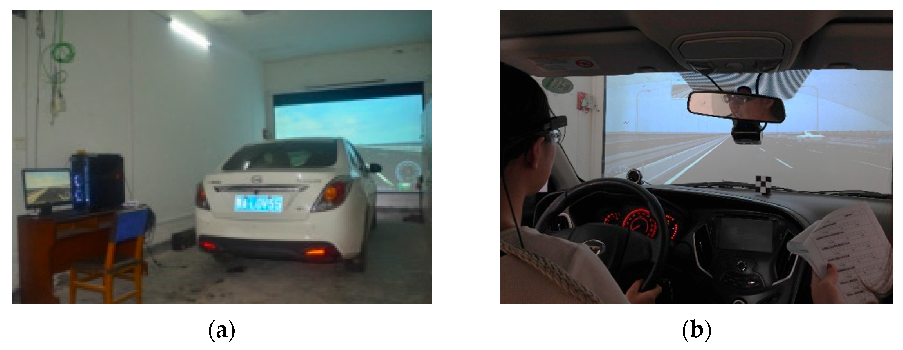
The simulated driving experiment was launched using the driving simulation platform shown in Figure 1. The driving simulation platform is located in the Intelligent Transportation System Research Center of the Wuhan University of Technology. It is a single-channel projection simulator consisting of a modified real vehicle and the UC-win/Road software. The software provides a rich set of editable traffic scenarios, which can be used to create virtual driving scenarios easily and rapidly. We used this software to create simulated driving scenarios. For driving data transmission, we gathered experimental vehicle data over the controller area network (CAN) bus and then provided it to the aforementioned software as input for driving operation behavior. This was accomplished with the aid of our self-developed SDK plugin.

The NASA-TLX scale is a multidimensional evaluation tool that assesses participants’ workload in six key areas: mental demand, physical demand, temporal demand, performance, effort, and frustration. It is the most frequently used instrument for measuring psychological load and is widely employed in performance research. According to related research, the NASA-TLX scale offers higher sensitivity than the majority of comparable tools, has good reliability, and has the potential to more accurately represent workload [28].

3.3. Experiment Design

This experiment controls four factors of the driving environment, including horizontal curve radius, longitudinal slope gradient, traffic flow, and sign information. We designed the scenarios according to the L₁₆(4⁵) orthogonal table shown in

Table 1. Orthogonal test factors.

Test Section	Factor
	Error Term	Radius (m)	Grade (%)	Flow (pcu/(h·ln))	Sign Information
1	4	300	−0.50%	700	C
2	2	700	−5.50%	700	A
3	4	2400	−5.50%	1070	B
4	3	700	−0.50%	1400	B
5	1	1500	−2.50%	700	B
6	4	700	−2.50%	230	D
7	1	700	−4.50%	1070	C
8	3	300	−2.50%	1070	A
9	1	300	−5.50%	1400	D
10	3	1500	−5.50%	230	C
11	2	300	−4.50%	230	B
12	2	1500	−0.50%	1070	D
13	3	2400	−4.50%	700	D
2	2	2400	−2.50%	1400	C
11	4	1500	−4.50%	1400	A
12	1	2400	−0.50%	230	A

and expected to obtain 16 experimental scenarios [29]. The simulated driving software UC-win/Road was used to conduct the scenario construction and simulation experiments. The simulated driving experiment road is a highway with a design speed of 100 km/h and a lane width of 3.75 m, in line with the specifications of the Highway Engineering Technical Standard (JTG B01-2014) (in China). It is situated in the plain microhill region and has four lanes going in both directions. The subjects’ workloads were measured using the NASA-TLX scale and driving performance data were collected using UC-win/Road simulation software.

3.4. Procedure

The staff asked the subjects some questions about their background and current health state before the experiment started, after which they explained the use of the driving simulator and the NASA-TLX scale [30]. They next arranged for the subjects to perform adaptive training to ensure that they were competent and could make accurate evaluations. Afterward, the staff confirmed that the subjects had no adverse reactions during the exercise.

To exclude interference, all individuals in the room turned off their communication devices before the formal experiment began. Unrelated people were asked to leave the laboratory. Subjects were asked to maintain their driving habits as in a real car as much as they could. The staff notified the subject of the trip’s destination before inviting them to the experiment section. They then asked the subject to determine the direction of the destination after successfully recognizing the traffic signs. After completing the driving task of one experimental scenario, the subject drove the vehicle into the transition section, completed the NASA-TLX scale with the assistance of the staff, and then drove into the next section. The experiment was limited to 90 min, thus avoiding fatigued driving.

The driver could only drive once in the scenario after the experiment formally started. The team arranged the cases in a random sequence to prevent learning effects. If a traffic accident occurred during driving, the subject was forced to take a 20-min break before continuing; if two driving accidents occurred, the experiment was terminated, and this subject was excluded from the experiment.

3.5. Data Processing

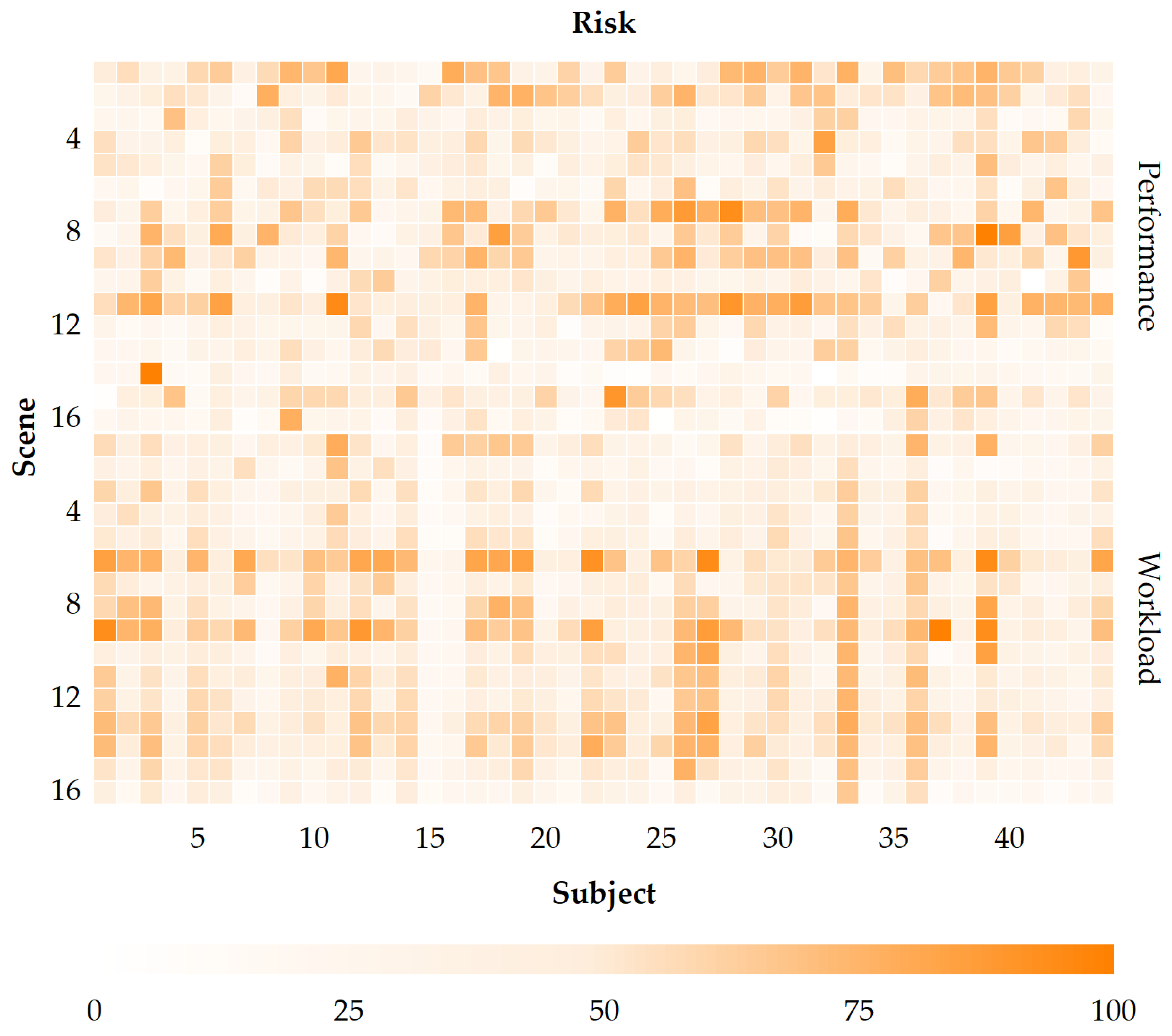
The input parameters of the evaluation model are divided into three categories, namely, driving environment, driving performance, and driving workload. Among them, the driving environment parameters were preset in the simulator during the scenario-building stage. Driving performance data were provided by the driving simulator. During the experiment, the driving simulator captured and preserved real-time driving performance data at a frequency of 10 Hz. These data could be exported after the experiment was completed. Driving workload data were provided by the NASA-TLX scale completed by the subjects. After obtaining the raw experimental data, we processed them to obtain data matrices.

3.5.1. Driving Performance

We filtered and extracted all driving performance data from the output data of the driving simulator and stored them in a table. We then segmented these time-series data by scenario and removed the data for nonexperimental road segments.

In this paper, we applied the DBSCAN algorithm to determine outliers and preprocess the driving performance data. DBSCAN (density-based spatial clustering of applications with noise) is a clustering method based on the density of sample points that determines the core points by taking into account the connectivity of a sample with other sample points in its neighborhood. To be considered core points, each sample point’s neighborhood must have $MinPts$ (minimal sample points) of samples within a specified $Eps$ (minimum radius) [31]. $Eps$ and $MinPts$ are artificially set. We chose the Mahalanobis distance as the distance measure between two points because it has two advantages [32]. One is that it excludes the interference of correlation between variables. Second, it eliminates the influence of the dimensions. Therefore, it enables us to effectively treat the driving performance variables.

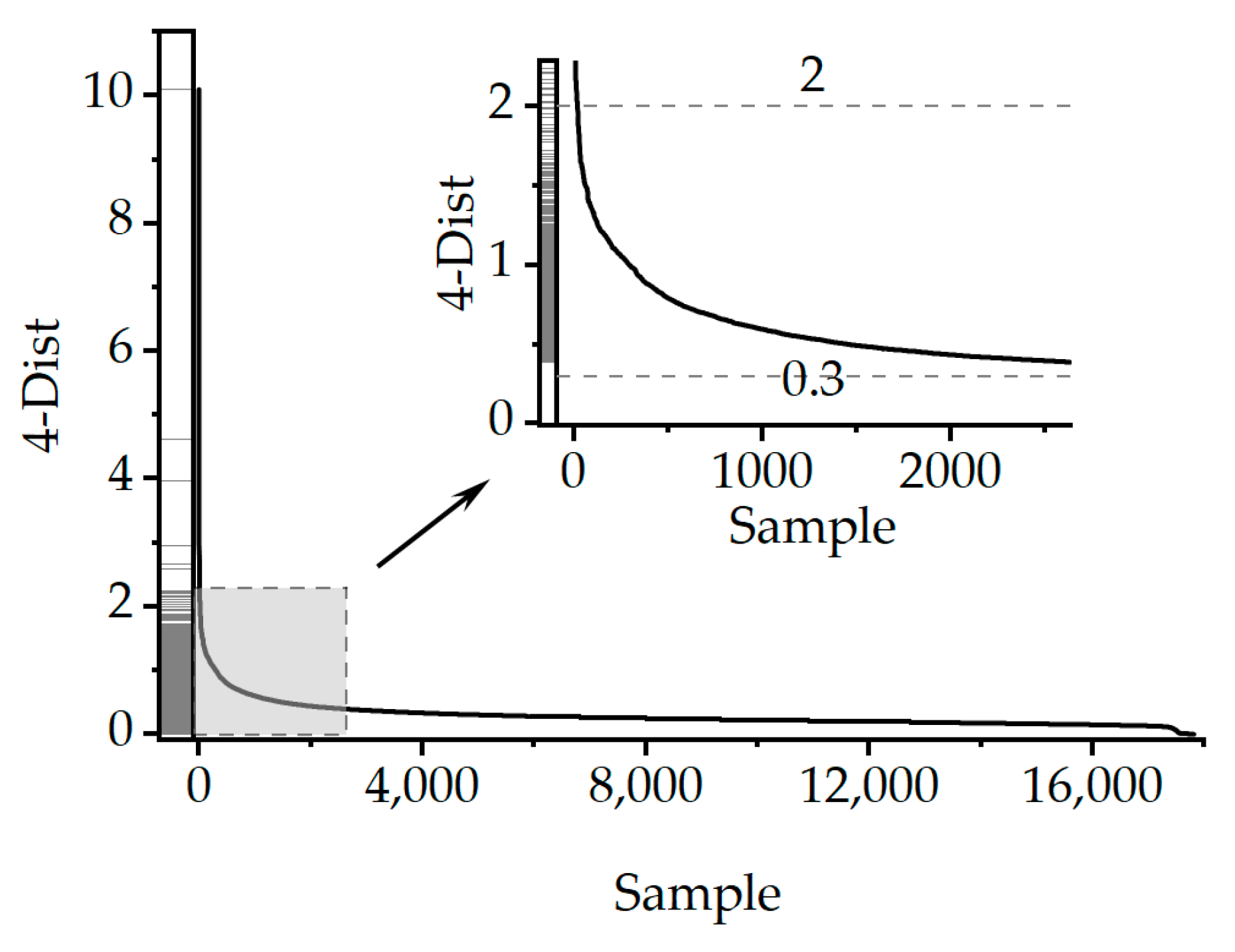
We applied the 4-dist chart to determine the two key parameters of the DBSCAN algorithm: $Eps$ and $MinPts$. The 4-dist, as well as the K-dist, chart is a method in [31] to determine these two parameters of the cluster in the database. The results of the experiment indicate that the 4-dist and the K-dist charts are not significantly different. Therefore, we set $MinPts$ to 4 and determined the $Eps$ by interaction using the 4-dist chart.

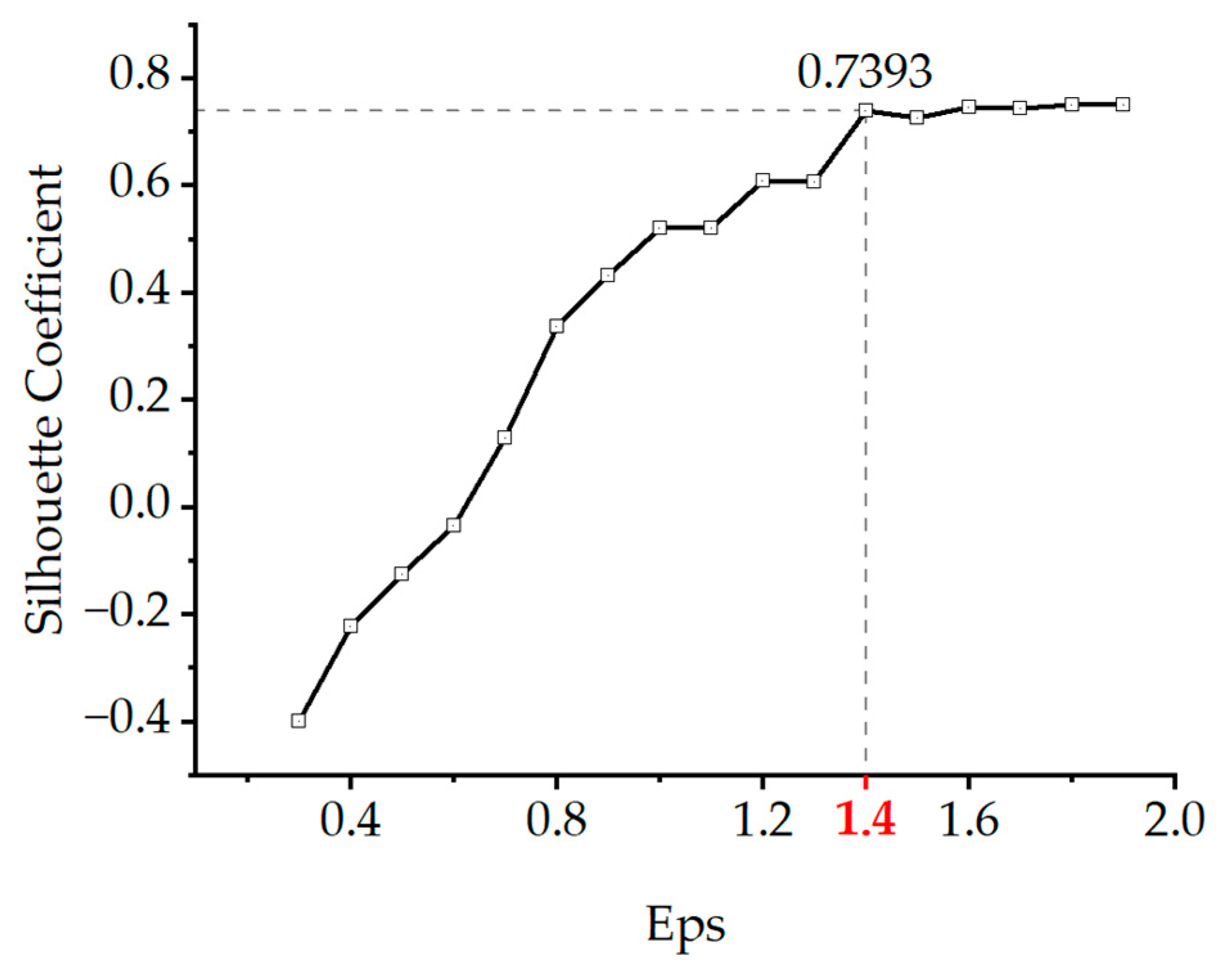
The 4-dist chart in Figure 2 shows the optimal $Eps$ for driving performance to be [0.3, 2]. We set $Eps=0.3$ and performed DBSCAN iterations in steps of 0.1. The calculation results are shown in Figure 3.

The silhouette coefficient is an evaluation method of clustering validity. The closer its value is to 1, the better the clustering effect [33]. As seen from Figure 3, the upward trend of the silhouette coefficient is no longer obvious for $Eps>1.4$. Thus, we set the parameters of DBSCAN $Eps=1.4$ and $MinPts=4$. After completing the parameter settings, we applied the DBSCAN algorithm to filter out the outliers. Then, we calculated the mean values of each driving performance parameter separately by scenario number. By calculation, we obtained the driving performance matrix $X_p$.

3.5.2. Driving Workload

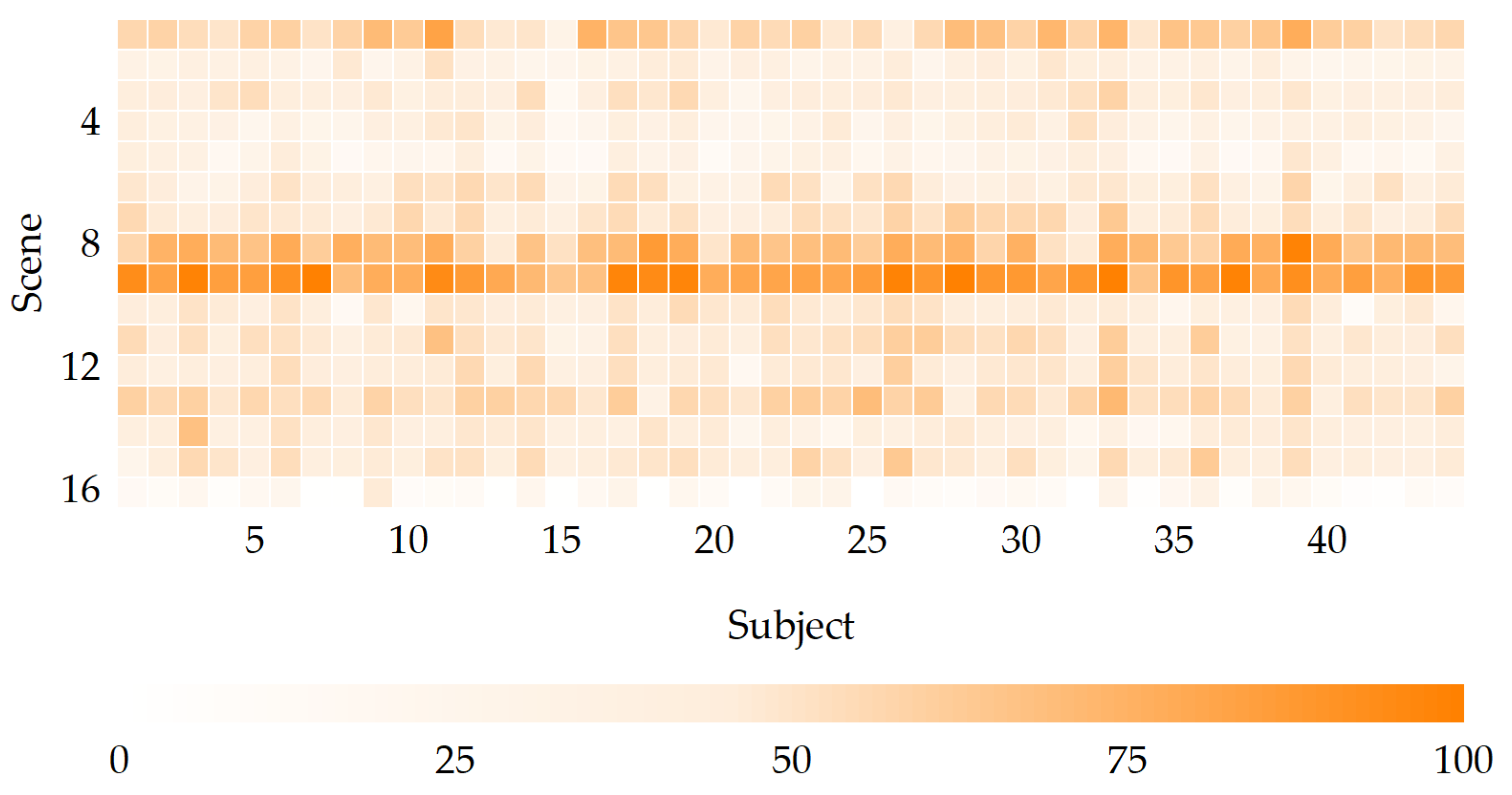
For the driving workload, we stored the measured NASA-TLX scale data in a table and calculated the weights $w_i$ based on the results of its second part (matching part). Then, we multiplied the scores ${\mathrm{Score}}_i$ of the six driving workload dimensions in the first part of the scale with their corresponding weights and calculated the weighted total score to obtain the driving workload $s$.

$$s=\frac{{{\displaystyle \sum }}_1^6{\mathrm{Score}}_i\times w_i}{100}$$

(1)

4. Methodology

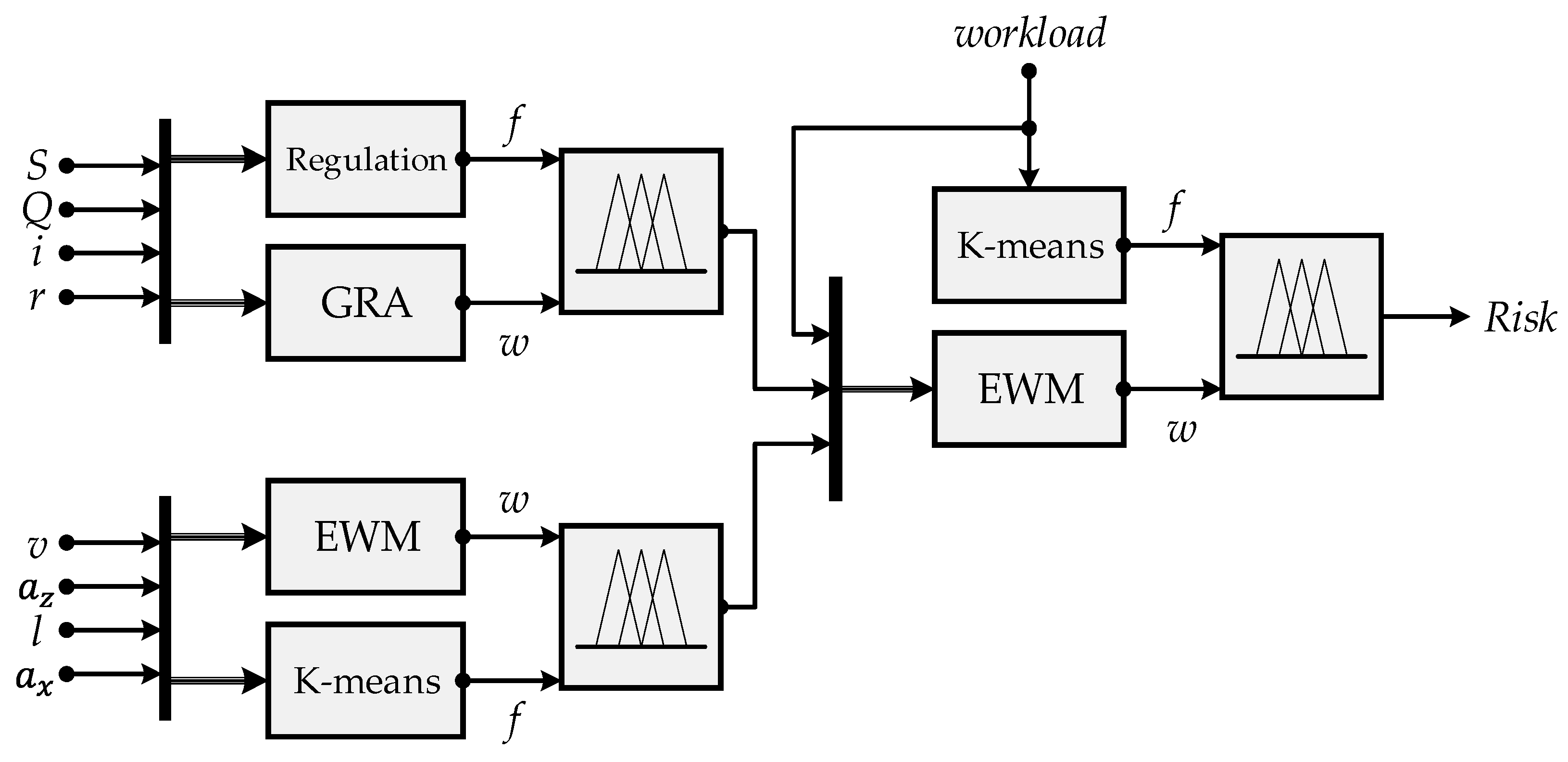
This section provides a detailed explanation of the steps involved in building the driving risk evaluation model. The modeling scheme is roughly divided into the following steps. First, we set up index sets and evaluation sets. Then, we constructed the membership functions and determined the index weights. Finally, we developed the fuzzy comprehensive evaluation model. Figure 4 depicts the general structure of the comprehensive evaluation scheme of driving risk.

4.1. Index Sets

Driving environment indices reflect the characteristics of the highway environment and the effects of static and dynamic factors on traffic safety. Road alignment can directly affect driving performance. On road sections with smaller horizontal curve radii, drivers need to carefully adjust the vehicle’s attitude to ensure that the vehicle passes through the curve safely [34]. When driving on longitudinally sloped sections, drivers need to ensure vehicle dynamics by constantly adjusting the accelerator and brake pedals [35]. The longitudinal slope increases the difficulty of vehicle control and the risk of collision. Drivers spend significantly less time maneuvering on curved and longitudinal slope sections, which increases the probability of accidents. One reasonable explanation is that more attention and mental resources are needed to obtain road information and make decisions [30,36].

The majority of researchers believe that as traffic volume increases, the crash rate also increases [37]. Fitzpatrick investigated the connection between driving performance and traffic flow using drivers’ cognitive time [38]. Compared to free driving, the severity of lateral conflict during lane changes rises with traffic flow, which undoubtedly increases the collision risk [39]. There is a threshold on the information of individual traffic signs. As the information on traffic signs grows, the driver’s cognitive time increases significantly, which shrinks the driver’s decision and maneuvering time [40,41]. Lyu et al. conducted a comprehensive analysis of the amount of traffic sign information to achieve information quantification and grading [24]. Based on information analysis for a large number of traffic signs, they classified the amount of traffic sign information into 4 levels. In this paper, we applied the above method to quantitatively classify the information on traffic signs and implement quantitative loading of driving workload for drivers in different scenarios.

Driving performance indices reflect the vehicle’s operation status and its dynamic performance [42]. According to studies, the vehicle speed is positively correlated with the traffic accident rate within a certain speed interval [43]. Therefore, the risk of traffic accidents increases as the operating speed increases. Longitudinal acceleration characterizes the fluctuation of the speed and can reflect the stability and safety of the vehicle in the longitudinal direction of the road [44]. Its variation is positively correlated with the traffic accident rate and can reflect the risk of driving to some extent. The lateral offset is the deviation of the longitudinal centerline of the vehicle from the centerline of its lane, which can reflect the lane keeping of the vehicle. Studies have shown that visual distractions during driving could lead to an increase in the lateral offset, thus causing driving risks [45]. Lateral acceleration is the acceleration perpendicular to the direction of travel when the vehicle is moving. It reflects the driver’s manipulation of the steering wheel and is often used to evaluate driving stability and comfort. Curve section driving is the root cause of lateral acceleration. As lateral acceleration increases, the risk of skid increases, which increases the possibility of accidents to some extent [34].

In addition, driving behavior is also affected by the workload experienced by the driver. According to the definition of mental workload, it is influenced by the driving task, driving environment, and driving experience and can reflect the driver’s attention resources during the driving task [46]. The driving workload and accident rate follow a U-shaped curve, indicating that there is no linear relationship between them. Accident rates under low or high driving workload conditions are higher than those under reasonable intervals [47].

In this paper, we considered the influence of the driving environment, driving performance, and driving workload on driving risk and selected nine indices from the above three aspects to build the index system. The related variables are shown in

Table 2. Variable descriptions.

Item	Symbol	Description	Unit
Environment	r	horizontal curve radius	m
	i	longitudinal slope gradient	%
	Q	traffic volume	pcu/(h·ln)
	S	traffic sign information	bit
Performance	v	vehicle speed	km/h
	$a_z$	vehicle longitudinal acceleration	$\mathrm{m}/{\mathrm{s}}^2$
	l	offset from the lane center	m
	$a_x$	vehicle lateral acceleration	$\mathrm{m}/{\mathrm{s}}^2$
Workload	s	driving workload measured by the NASA-TLX scale	%
Risk	$Ris{k}_e$	driving risk determined by factors of driving environment	%
	$Ris{k}_p$	driving risk related to vehicle dynamics parameters	%
	Risk	comprehensive driving risk determined by such factors as people, vehicles, and road environment	%

.

4.2. Evaluation Sets

The evaluation sets and membership functions of each index must be determined to construct a comprehensive evaluation model. The evaluation sets and membership functions of $\left\{r,i,Q,S,v\right\}$ are determined according to the Road Traffic Safety Law of the People’s Republic of China and the Technical Standard of Highway Engineering (JTG B01-2014). Since indices such as $\left\{a_z,l,a_x,s\right\}$ lack the classification criteria of the evaluation level, this paper applied the k-means clustering algorithm to construct their evaluation system.

The purpose of clustering is to group all samples into a finite number of clusters and extract intervals of different evaluation levels of each index to construct a fuzzy evaluation matrix. The k-means algorithm is one of the most widely used clustering algorithms and is efficient and easy to implement. Here, we determined the sample point distances using the Euclidean method to calculate the sum of squared distances between each cluster’s center point ${\mu }_i$ and points inside it. The algorithm performs the iterative calculation on the data, stops the operations when a given accuracy is reached, and outputs the clustering results to minimize the total sum of $J$ squares for each cluster.

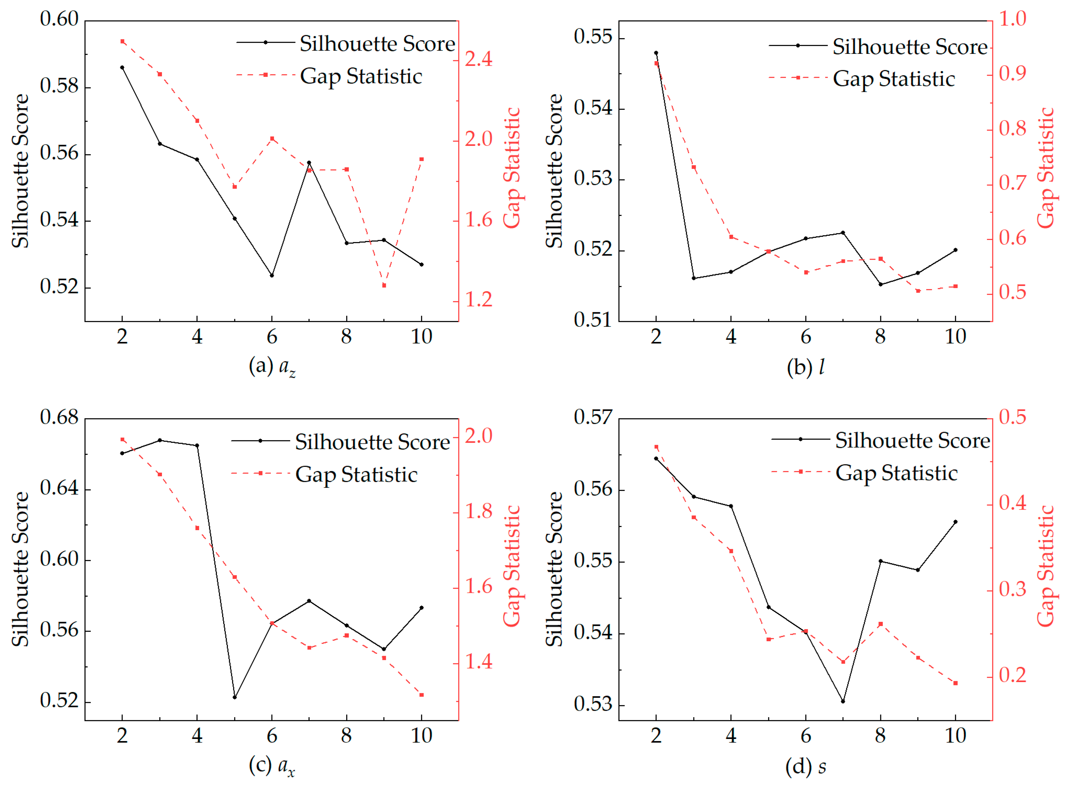
Since the data we obtained were not labeled, we chose internal indices to evaluate the clustering effect as a way to select $K$ when the indices are optimal. Here, we chose the silhouette coefficient for evaluation and verified this optimal value by referring to the gap statistic algorithm [33]. The gap statistic algorithm finds $K$ that makes $Gap\left(K\right)$ reach the maximum by calculating the sum of squares’ distances inside the cluster [48]. Under this condition, the difference between the random sample loss and the actual sample loss reaches the maximum.

Figure 5 shows the silhouette coefficients and $Gap\left(K\right)$ of each index for different $K$. As seen from the figure, the optimal $K$ values corresponding to $\left\{a_z,l,a_x,s\right\}$ are $\left\{2,2,3,2\right\}$. Considering that there is not much of a difference between $K=2$ and $K=3$, setting $K=3$ is more favorable for the construction of the membership functions; hence, their $K$ values were taken to be 3. Thus, the $K$ values of each index were determined as $\left\{3,2,3,3\right\}$. 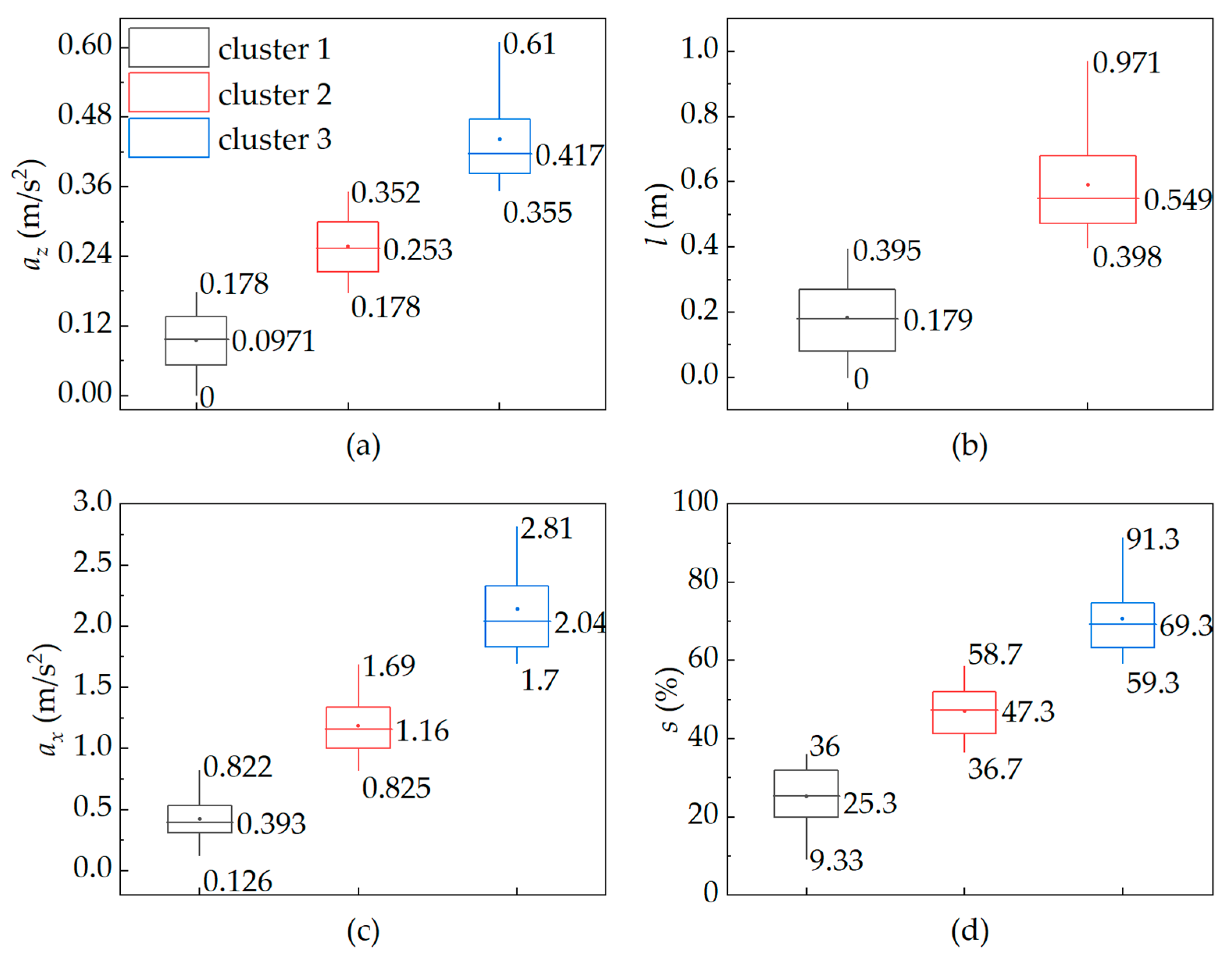The clustering results are shown in Figure 6.

4.3. Membership Functions

Based on the above results, the evaluation set and membership functions for each index were constructed. Considering the differences in attributes among indices, we used a combination of the triangular membership function and trapezoidal membership function to construct the membership functions of the comprehensive evaluation model. They are similar to Figure 7.

This approach can reflect the differences between different indices while ensuring high sensitivity of the input and output variables [42]. Here, we applied the results of the K-means clustering analysis described above to define the clusters of indices that were categorized using the corresponding evaluation levels. We defined the upper and lower limits of each cluster as the segmented nodes of the corresponding membership function, thus achieving differential construction. The completed membership functions were constructed as shown in

Table 3. Index membership functions.

Safety Level	Membership Functions
	Indices Except for $\mathit{v}$	$\mathit{v}$
Good	$f\left(x\right)=\left\{\begin{array}{ll}\hfill 1,& \hspace{1em}a<x\le b\hfill \\ \hfill \frac{c-x}{c-b},& \hspace{1em}b<x\le c\hfill \\ \hfill 0,& \hspace{1em}x\ge c\hfill \end{array}\right.$	$f\left(x\right)=\left\{\begin{array}{ll}\hfill 0,& \hspace{1em}x\le b\hfill \\ \hfill \frac{x-b}{c-b},& \hspace{1em}b<x\le c\hfill \\ \hfill 1,& \hspace{1em}c<x\le d\hfill \\ \hfill \frac{e-x}{e-d},& \hspace{1em}d<x\le e\hfill \\ \hfill 0,& \hspace{1em}x>e\hfill \end{array}\right.$
Medium	$f\left(x\right)=\left\{\begin{array}{ll}\hfill 0,& \hspace{1em}x\le b\hfill \\ \hfill \frac{x-b}{c-b},& \hspace{1em}b<x\le c\hfill \\ \hfill \frac{d-x}{d-c},& \hspace{1em}c<x\le d\hfill \\ \hfill 0,& \hspace{1em}x\ge d\hfill \end{array}\right.$	$f\left(x\right)=\left\{\begin{array}{ll}\hfill 0,& \hspace{1em}x\le a\hfill \\ \hfill \frac{x-a}{b-a},& \hspace{1em}a<x\le b\hfill \\ \hfill \frac{c-x}{c-b},& \hspace{1em}b<x\le c\hfill \\ \hfill 0,& \hspace{1em}c<x\le d\hfill \\ \hfill \frac{x-d}{e-d},& \hspace{1em}d<x\le e\hfill \\ \hfill \frac{f-x}{f-e},& \hspace{1em}e<x\le f\hfill \\ \hfill 0,& \hspace{1em}x>f\hfill \end{array}\right.$
Bad	$f\left(x\right)=\left\{\begin{array}{ll}\hfill 0,& \hspace{1em}x\le c\hfill \\ \hfill \frac{x-c}{d-c},& \hspace{1em}c<x\le d\hfill \\ \hfill 1,& \hspace{1em}d<x\le e\hfill \end{array}\right.$	$f\left(x\right)=\left\{\begin{array}{ll}\hfill 1,& \hspace{1em}x\le a\hfill \\ \hfill \frac{b-x}{b-a},& \hspace{1em}a<x\le b\hfill \\ \hfill 0,& \hspace{1em}b<x\le e\hfill \\ \hfill \frac{x-e}{f-e},& \hspace{1em}e<x\le f\hfill \\ \hfill 1,& \hspace{1em}x>f\hfill \end{array}\right.$

. The nodes of each evaluation interval are represented by the parameters in Table 3, and

Table 4. Critical values of indices.

Index	a	b	c	d	e	f
$r$	2400	2400	700	400	300
$i$	0	−0.5	−2.5	−4	−5.5
$Q$	230	230	700	1400	1800
$S$	0	40	80	120	160
$a_z$	0	0.097	0.253	0.355	1
$l$	0	0.179	0.549	1	1.875
$a_x$	0	0.393	1.16	2.04	5
$s$	0	36	47.3	58.7	100
$v$	60	80	100	120	132	144

displays their corresponding values.

4.4. Weight System

Considering the differences in the importance of the foundation and superstructure indices, we calculated the index weights from the bottom to the top.

Previous studies have analyzed the correlation between driving workload, driving performance, and driving environment [49]. The gray relational characterizes the degree of correlation between indices and can reflect how important the participating indices are in comparison to the reference indices. From this, we can derive the weights of driving environment subordinate indices. Driving workload indices and driving performance indices can reflect the influence of driving environment factors on drivers’ driving behavior. This study chose the vehicle speed and driving workload to determine the weights for the driving environment index $W_e$.

For other indices, the entropy weight method (EWM) was used to calculate the weights. EWM is an objective weighting method that determines the weight by calculating the difference in the information entropy of indices. In essence, it assigns weights to indices by considering their discrete degree, which can more accurately reflect the extent to which indices such as the driving environment, driving performance, and driving workload affect the risk of highway driving. According to Shannon’s information entropy theory, we calculated the index weights by Equations (2)–(4) [50]. Unlike the concept of information entropy proposed by Shannon, the value of $a$ was taken here as the value of the number of evaluation objects involved in the weight calculation, instead of the default value of 2. This ensures a reasonable distribution of weights. This paper proposed a solution to the issue that zero values may appear after index normalization: whenever a particular index appears to be zero, all index values of the object involved in the weight calculation are increased by $1\times {10}^{-5}$. This ensures the data integrity to the maximum extent without affecting the weight distribution of indices.

$${\rho }_{ij}=\frac{x_{ij}^{\prime }}{{{\displaystyle \sum }}_{i=1}^k{x}_{ij}^{\prime }}$$

(2)

$$I_j=-{\displaystyle \sum }_{i=1}^k{\rho }_{ij}{\mathit{log}}_a({\rho }_{ij})$$

(3)

$$w_j=\frac{1-I_j}{{{\displaystyle \sum }}_{j=1}^m\left(1-I_j\right)}$$

(4)

where $x_{ij}^{\prime }$ is the normalized data, ${\rho }_{ij}$ is the proportion of $x_{ij}^{\prime }$ in index $q_j$, $I_j$ is the information entropy of the index, and $w_j$ is the weight of index $q_j$. We obtained the index weight vector $W_p$ using the aforementioned calculation. Based on the weight determination method in the previous section, we calculated the index weights separately.

Table 5. Index weights of the foundation.

Item	Index	Weight
ENVIR	$r$	0.218
	$i$	0.211
	$Q$	0.28
	$S$	0.291
PERF	$v$	0.284
	$a_z$	0.173
	$l$	0.248
	$a_x$	0.295

displays the derived driving performance index weights $W_p$ and driving environment index weights $W_e$.

After completing the foundation evaluation, we obtained the risk values of the foundation evaluation for each subject. By integrating the foundation evaluation results into vector form, we obtained the driving performance risk vector $S_p$ and the driving environment risk vector $S_e$. Next, using Equation (5), we integrated $S_p$, $S_e$, and the driving workload vector $s$ to obtain the superstructure’s weighting matrix $X$. To obtain the index weights $W$ for the superstructure evaluation, we normalized the weighting matrix $X$ and computed the index weights by the previously discussed EWM (Equations (2)–(4)). The calculation results are shown in

Table 6. Index weights of the superstructure.

Index	Weight
$Ris{k}_e$	0.304
$Ris{k}_p$	0.268
$s$	0.428

. Thus, we completed the construction of the model weight system.

$$X=\left(S_p,S_e,s\right)={\left[\begin{array}{ccc}Ris{k}_{p1}& Ris{k}_{e1}& s_1\\ Ris{k}_{p2}& Ris{k}_{e2}& s_2\\ ⋮& ⋮& ⋮\\ Ris{k}_{pk}& Ris{k}_{ek}& s_k\end{array}\right]}_{k\times 3}={\left[\begin{array}{ccc}{x}_{11}& x_{12}& x_{13}\\ x_{21}& x_{22}& x_{23}\\ ⋮& ⋮& ⋮\\ x_{k1}& x_{k2}& x_{k3}\end{array}\right]}_{k\times 3}$$

(5)

4.5. Fuzzy Comprehensive Evaluation Model

Let there be $m$ different risk factors in total, which are represented by $q_1, q_2, \cdots ,q_m$; then, there are $m$ indices of the comprehensive evaluation model corresponding to these influencing factors, and let the index set be $Q=\left\{q_1, q_2, \cdots , q_m\right\}$. The levels corresponding to the indices vary among them. Let the index $q_i$ have $n$ levels; then, the index has $n$ evaluation levels. The evaluation levels are $v_1, v_2, \cdots , v_n$, and the evaluation set is $V=\left\{v_1, v_2, \cdots , v_n\right\}$.

Let $u_j$ be the membership function of index $q_i$ in level $v_j$; then, $u_j=\mu \left(v_j\right)$, $U=\left\{u_1, u_2, \cdots , u_n\right\}$. From this, we calculated the risk evaluation matrix $R_{m\times n}$ based on the membership function, where $r_{ij}=u_j\left(q_i\right)$.

After obtaining the evaluation matrix $R$ and the index weight vector $W$, we performed a comprehensive evaluation layer by layer from the bottom to the top and calculated the driving performance risk vector $Ris{k}_p$ and the driving environment risk vector $Ris{k}_e$. As shown in Equation (6), the comprehensive evaluation operation $\Delta -\nabla$ used the (${⨁}_{\epsilon }$,${⨂}_{\epsilon }$) operator. This strategy retains the evaluation information of individual indices while taking into account the overall effect [51].

$$e_j=R\circ W=\left(r_{1j}\nabla w_1\right)\Delta \left(r_{2j}\nabla w_2\right)\Delta \cdots \Delta \left(r_{mj}\nabla w_m\right)$$

(6)

where $e_j$ is the degree to which the indices are affiliated in level $j$. In this paper, $f$ was defined as the quantitative matrix corresponding to the evaluation levels of indices. From this, we calculated the fuzzy comprehensive evaluation values $Ris{k}_p$ and $Ris{k}_e$ according to Equations (7)–(10).

$$e_j^{\prime }=\frac{e_j}{{{\displaystyle \sum }}_{j=1}^n{e}_j}$$

(7)

$$E^{\prime }=\left(e_1^{\prime },e_2^{\prime },\cdots ,e_n^{\prime }\right)$$

(8)

$$f=100·\left(1,\frac{n-1}{n},\frac{n-2}{n},\cdots ,\frac{1}{n}\right)$$

(9)

$$Risk=E^{\prime }·f^T$$

(10)

We substituted $s_i$ into the corresponding membership functions and applied Equation (11) to obtain the superstructure evaluation matrix $R$. According to Equations (6)–(10), we integrated $R$, $W$, and $f$ to obtain the comprehensive evaluation value of driving risk $Risk$. Finally, we obtained the evaluation model of driving risk.

$$R=\left[\begin{array}{c}{E}_p\\ E_e\\ E_s\end{array}\right]={\left[\begin{array}{cccc}{e}_{11}& e_{12}& \cdots & e_{1n}\\ e_{21}& e_{22}& \cdots & e_{2n}\\ e_{31}& e_{32}& \cdots & e_{3n}\end{array}\right]}_{3\times n}$$

(11)

5. Results

In the following, we present the evaluation results of the model. We constructed a two-layer TOPSIS model for comparison and calculated the evaluation results using the same input dataset. Finally, we compared the evaluation results of these two methods to verify the validity of the model.

5.1. Evaluation Results

Figure 8 is divided into two parts, showing the assessment values of driving performance $Ris{k}_p$ and driving workload $s$ for each subject. The 44 subjects’ comprehensive risk of driving performance in 16 scenarios comprise the top section, while their driving workload scores $s$ are depicted in the bottom part. $Ris{k}_p$ was determined by comprehensive assessment $\left\{v,a_z,l,a_x\right\}$. Heatmaps are used to display the evaluation results. Each square in the graph corresponds to a subject (horizontal coordinate) and a scenario (vertical coordinate). The color of the squares is used to indicate the driving performance risk (top) and driving workload (bottom) in a given scenario. In other words, the color depth of the blocks serves as an indicator of the risk values. The legend indicates that the color of the relevant square changes depending on the risk value: the greater the risk value is, the darker the color; the lower the risk value is, the closer the color is to white. It is clear that the model is capable of easily identifying scenarios with high driving performance risk and high driving workload. As seen from the figure, despite the high subjective driving load of drivers in some scenarios (e.g., segments 6 and 9), there was no deterioration in driving performance.

Figure 9 shows the evaluation results of each subject, that is, the value of driving risk, $Risk$, which is obtained from the comprehensive evaluation of three variables $\left\{Ris{k}_e,Ris{k}_p,s\right\}$. It shows the comprehensive driving risk of the 44 subjects in 16 different scenarios in the form of a heatmap. As with the foundation evaluation, the comprehensive driving risk values are marked in the form of color depth, and the correspondence rules are the same. The figure illustrates that the model is able to clearly detect high-risk driving scenarios. As observed from the figure, the driving risk in these complicated scenarios (e.g., segments 8 and 9) is obviously higher than that of other sections. Compared with the assessment based on behavior or workload alone, the comprehensive assessment results of risk show a similar trend for each participant.

5.2. Model Validation

To verify the effectiveness of the proposed method in this paper, we constructed a TOPSIS model for comparison. The TOPSIS model can be used to evaluate each solution by calculating the distance between the evaluation object and the ideal solution. This method can make full use of the original data with little information loss and works well to resolve the multi-index decision problem. Similar to the method proposed in this work, the TOPSIS model we built is divided into two evaluation structures. The calculation process is as follows.

First, we normalized and standardized the data of each index and then integrated them to construct the evaluation matrix $Z_{k\times m}$. Equation (12) illustrates the process of standardization.

$$z_{ij}=\frac{x_{ij}}{\sqrt{{{\displaystyle \sum }}_{i=1}^k{x}_{ij}^2}}$$

(12)

We determined the positive ideal solution $Z^{+}$ and the negative ideal solution $Z^{-}$ of the matrix $Z$. $Z^{+}$ is the vector consisting of the optimal values of each column of $Z$, and $Z^{-}$ is the vector consisting of its worst values. Since we normalized the data, the optimal value is the maximum value of each column, and the worst value is its minimum value. The representation of $Z^{+}$ and $Z^{-}$ is shown in Equations (13)–(14).

$$Z^{+}=\left[z_1^{+},z_2^{+},\cdots ,z_m^{+}\right]$$

(13)

$$Z^{-}=\left[z_1^{-},z_2^{-},\cdots ,z_m^{-}\right]$$

(14)

where $z_m^{+}=max\left\{z_{1m}, z_{2m}, \cdots , z_{km}\right\}$, $z_m^{-}=min\left\{z_{1m}, z_{2m}, \cdots , z_{km}\right\}$. Accordingly, we calculated the evaluation object’s distance $d_i^{+}$ from the positive ideal solution $Z^{+}$ and its distance $d_i^{-}$ from the negative ideal solution $Z^{-}$. The calculation process is shown in Equations (15)–(16). Finally, we evaluated the solution by calculating the similarity $C$ of each evaluation object to the ideal solution by Equation (17).

$$d_i^{+}=\sqrt{{\displaystyle \sum }_{j=1}^m{w}_j{\left(z_j^{+}-z_{ij}\right)}^2}$$

(15)

$$d_i^{-}=\sqrt{{\displaystyle \sum }_{j=1}^m{w}_j{\left(z_{ij}-z_j^{-}\right)}^2}$$

(16)

$$C_i=\frac{d_i^{-}}{d_i^{+}+d_i^{-}}$$

(17)

The TOPSIS model evaluation integrates three aspects: driving environment, driving performance, and driving workload. This makes it possible to assess the comprehensive driving risk. The driving environment index and driving performance index are the results of the foundation evaluation in TOPSIS. We calculated the similarity $C$ of the comprehensive driving risk of each subject in different scenarios. A higher value of $C$ indicates a higher risk. Figure 10 shows the analysis results of the comprehensive driving risk. By comparison, we can see that the assessment results of these two methods are basically the same. However, this conclusion remains to be tested.

We used the two-sample K-S test to test the evaluation results. The test findings indicate that there was no statistically significant difference between the two samples (Z = 1.119, p = 0.163). The null hypothesis is accepted with p > 0.05. In other words, the distributions of the assessment results for the two methods are the same. Pearson correlation analysis was used to test the evaluation results of these methods, and the test results show a significant positive correlation between them (r = 0.824, p < 0.01). This further verifies the effectiveness of the method proposed in this work.

6. Conclusions

This work proposes a fuzzy mathematics-based method for assessing the risk of highway driving. It achieves risk evaluation in the process of driving and is able to evaluate the effect of each influencing factor on driving risk. Its main contribution is the realization of comprehensive measurement and assessment of highway driving risk.

The model integrates data from three aspects: driving environment, driving performance, and driving workload. The evaluation system is constructed by clustering, and the weight system is constructed by the entropy weight method and gray relational analysis. The model is divided into two layers. Driving environment data and driving performance data were collected and provided by the driving simulator and driving workload data were obtained based on the NASA-TLX scale. As a comparison, we also constructed a two-layer TOPSIS model and tested the evaluation results. The test showed a significant positive correlation between the results. Thus, the validity of the model was verified. The findings demonstrate that the proposed method can accurately measure driving risk.

The method provided in this study has certain advantages. It characterizes the risk of the human factors in terms of the driving workload, which provides a more comprehensive consideration of driving risk. In addition, it does not require additional equipment in the data measurement process and the required data can be provided by vehicle sensors and scales. This facilitates the application of the model in real driving conditions. Road traffic safety is influenced by various factors, which may be correlated with each other. Optimization of the index system of the model, traffic safety facilities, and improvement measures for traffic safety management will be the focus of future research.