A Method of Reducing Invalid Steering for AUVs Based on a Wave Peak Frequency Tracker

Abstract

The motion control of autonomous underwater vehicles (AUVs) is affected by waves near the ocean surface or in shallow-water areas. Therefore, to counteract the influence of waves, we need to remove them by designing a filter. The wave peak frequency is important in wave filter design. This paper focuses on the identification of the wave peak frequency using the least-squares parameter estimation algorithm. The input–output expression of the wave disturbance model is derived by eliminating the intermediate variable. Based on the obtained identification model, an auxiliary model-based recursive extended least-squares identification algorithm is developed to estimate the model parameters. The effectiveness of the proposed method is verified with simulated tests of the heading control system of an AUV. The simulation results demonstrate that the proposed method is effective for the identification of the wave peak frequency, and an observer with a wave peak frequency tracker can significantly reduce invalid steering.

1. Introduction

In recent years, AUVs have been widely applied in more and more scenarios near the ocean surface and in shallow-water areas, such as in sea-bottom surveys, undersea pipe maintenance, hydrographic surveys, and so on [1]. However, when an AUV is sailing near the ocean surface or in shallow-water areas, the forces and moments induced by waves have a great influence on its maneuvering characteristics and postures [2]. Over the last decades, there has been an increasing demand for higher accuracy and reliability in the motion control systems of AUVs. A wave filter is a simple and effective way to improve the performance of the motion control system of an AUV [3]. An accurate description of wave disturbances is important in the design of a motion control system for an AUV. There are many different nonlinear models for describing the wave spectra under different sea states, such as the Neuman spectrum, Bretschneider spectrum, Pierson–Moskowitz (PM) spectrum, Modified PM spectrum, JONSWAP spectrum, etc. [4]. Due to the complexity of the nonlinear models of wave spectra, linear models have been introduced to approximate them [5]. Among them, the second-order wave disturbance state-space model was employed to fit the PM spectrum, and this has had extensive applications [6].

In the last decades, model-based methods of controller design, observer design, and system analysis [7,8,9] have received much attention. System identification theory has been applied in order to establish a model that is close to a real system by using the obtained input–output data [10]. Numerous identification methods have been developed for the modeling of linear systems [11,12,13] and nonlinear systems [14,15,16]. Wang et al. proposed a recursive least-squares identification method based on the filtering of input–output data for controlled autoregressive moving-average systems [17]. Xiao et al. presented a filtering-based least-squares algorithm for input nonlinear dynamical adjustment models using a data-filtering technique [18].

Based on the classification of off-line and on-line parameter estimation, least-squares algorithms can be divided into iterative least-squares-based algorithms [19,20,21,22] and recursive least-squares algorithms [23,24,25]. Wang et al. studied the identification of parameters for multivariable Hammerstein systems based on an improved least-squares algorithm [26]. Chen et al. developed a decomposition-based recursive least-squares algorithm for input nonlinear controlled autoregressive input systems [27]. For a class of identification models in the presence of unmeasurable variables in information vectors, an auxiliary model can be employed [28,29,30]. Its main idea is to replace the unknown items with their corresponding estimates [31]. Guo et al. derived a recursive least-squares algorithm for bilinear stochastic systems with colored noise by combining the idea of auxiliary model identification and the principle of hierarchical identification [32]. Wang et al. proposed a recursive least-squares algorithm for linear-in-parameters output moving average systems using the idea of auxiliary model identification [33].

The wave-filtering technique is important for the motion control system of an AUV near the ocean surface due to its ability to separate heading measurements into low-frequency (LF) and high-frequency (HF) components [34,35]. Generally, the LF components are effective signals for the motion control systems of AUVs. The HF components (i.e., wave-frequency motion) can aggravate the invalid steering of AUVs, which leads to actuator wear, fuel consumption, and emissions. Therefore, the HF components should be prevented from entering the control loop. To eliminate the influence of the HF components of a wave, a wave filter for marine vehicles with a gain-scheduled method was presented in the literature [36]. Wang et al. designed an extended state observer to prevent high-frequency wave disturbances from entering the controller [37]. Hassani et al. introduced an adaptive wave filter based on multiple models to eliminate wave disturbances [38]. The wave peak frequency is critical for wave filter design [39]. However, the peak frequency of a wave spectrum varies with the sea state and the navigation state of the AUV, making it difficult to obtain the accurate wave peak frequency [40]. In recent decades, numerous methods have been presented for the identification of the wave peak frequency. Bryne et al. presented a strapdown inertial navigation system with adaptive wave filtering for a ship motion control system by using a signal-based frequency tracker [41]. Hassani et al. proposed an adaptive wave filter composed of a recursive optimization procedure that sought to identify the dominant wave frequency by minimizing an appropriately defined performance index [42].

Based on the idea of auxiliary model identification, this paper presents an online parameter estimation method for identifying the wave peak frequency by using the recursive extended least-squares (RELS) algorithm. Based on the identified wave peak frequency, the gain vector of the observer is updated in real time, which effectively improves the performance of the observer. The simulation results indicate that the invalid steering of AUVs is significantly reduced with the proposed wave peak frequency tracker.

The remainder of this paper is organized as follows. Section 2 derives the input–output representation of the wave disturbance model. Section 3 presents the method of the design of the wave peak frequency tracker. The heading control system of the AUV is established in Section 4 to verify the effectiveness of the proposed method. The simulation results and an analysis are given in Section 5. The conclusions are described in in Section 6.

2. System Description and Identification Model

The state-space model of the HF wave disturbance components caused by the first-order-wave-induced forces can be expressed as:

$$\begin{array}{cc}\hfill \left[\begin{array}{c}{\dot{\zeta }}_{\varpi }\\ {\dot{\varphi }}_{\varpi }\end{array}\right]=& \left[\begin{array}{cc}0& 1\\ -{\varpi }_0^2& -2\xi {\varpi }_0\end{array}\right]\left[\begin{array}{c}{\zeta }_{\varpi }\\ {\varphi }_{\varpi }\end{array}\right]+\left[\begin{array}{c}0\\ K_{\varpi }\end{array}\right]v,\hfill \end{array}$$

(1)

$$\begin{array}{cc}\hfill y_{\varpi }=& \left[01\right]\left[\begin{array}{c}{\zeta }_{\varpi }\\ {\varphi }_{\varpi }\end{array}\right],\hfill \end{array}$$

(2)

where ${\varpi }_0$ denotes the wave peak frequency, ${\zeta }_{\varpi }$ denotes the wave state, ${\varphi }_{\varpi }$ denotes the HF heading component due to the first-order-wave-induced forces, v denotes the Gaussian white noise, $\xi$ is the relative damping ratio, and $K_{\varpi }$ is a constant describing the wave excitation intensity.

In order to derive the input–output expression of the wave disturbance model, the state-space model in (1) can be written as an autoregressive moving average (ARMA) model [4]:

$$\begin{array}{c}\hfill A\left(z^{-1}\right){\varphi }_{\varpi }\left(k\right)=B\left(z^{-1}\right)v\left(k\right),\end{array}$$

(3)

where

$$\begin{array}{cc}\hfill A\left(z^{-1}\right)& :=1+a_1{z}^{-1}+a_2{z}^{-2},\hfill \end{array}$$

(4)

$$\begin{array}{cc}\hfill B\left(z^{-1}\right)& :=1+b_1{z}^{-1}.\hfill \end{array}$$

(5)

On the basis of (1) and (3), we have the following relationship:

$$\begin{array}{cc}\hfill {\varphi }_{\varpi }\left(t\right)=& -a_1{\varphi }_{\varpi }(t-1)-a_2{\varphi }_{\varpi }(t-2)+b_{1}v(t-1)+v\left(t\right).\hfill \end{array}$$

(6)

However, in practice, the heading signal ${\varphi }_{tot}\left(s\right)$ measured by a compass contains an LF heading component $\varphi \left(s\right)$ and HF heading component ${\varphi }_{\varpi }\left(s\right)$ simultaneously, that is,

$$\begin{array}{c}\hfill {\varphi }_{tot}\left(s\right)=\varphi \left(s\right)+{\varphi }_{\varpi }\left(s\right).\end{array}$$

(7)

Hence, the HF heading component ${\varphi }_{\varpi }\left(s\right)$ cannot be directly obtained with the compass measurement. In order to separate the HF heading component ${\varphi }_{\varpi }\left(s\right)$ from the compass measurement ${\varphi }_{tot}\left(s\right)$, a high-pass filter $h_{HP}\left(s\right)$ could be employed by using a filtered signal ${\overline{\varphi }}_{\varpi }\left(s\right)$. Therefore, the approximation of ${\varphi }_{\varpi }\left(s\right)$ is given by

$$\begin{array}{c}\hfill {\overline{\varphi }}_{\varpi }\left(s\right)=h_{HP}\left(s\right){\varphi }_{tot}\left(s\right).\end{array}$$

(8)

If the following condition can be satisfied

$$\begin{array}{c}\hfill h_{HP}\left(s\right)\varphi \left(s\right)=h_{HP}\left(s\right)h_{ship}\left(s\right)u\left(s\right)\ll 1,\end{array}$$

(9)

then, the high-pass filter $h_{HP}\left(s\right)$ will undermine the LF heading component.

Replacing ${\varphi }_{\varpi }\left(s\right)$ with its approximate value ${\overline{\varphi }}_{\varpi }\left(s\right)$, Equation (6) can be rewritten as

$$\begin{array}{cc}\hfill {\overline{\varphi }}_{\varpi }\left(t\right)=& -a_1{\overline{\varphi }}_{\varpi }(t-1)-a_2{\overline{\varphi }}_{\varpi }(t-2)+b_{1}v(t-1)+v\left(t\right).\hfill \end{array}$$

(10)

Let y be equal to ${\overline{\varphi }}_{\varpi }$, and Equation (10) can be rewritten as

$$\begin{array}{cc}\hfill y\left(t\right)& ={\mathbf{\phi }}_s^T\left(t\right){\mathbf{\theta }}_s+{\phi }_n\left(t\right){\theta }_n+v\left(t\right)\hfill \end{array}$$

(11)

$$\begin{array}{cc}\hfill & ={\mathbf{\phi }}^T\left(t\right)\mathbf{\theta }+v\left(t\right),\hfill \end{array}$$

(12)

where

$$\begin{array}{cc}\hfill {\theta }_n& :=b_1,\hfill \\ \hfill {\mathbf{\theta }}_s^T& :=[a_1,a_2],\hfill \\ \hfill {\mathbf{\theta }}^T& :=[{\mathbf{\theta }}_s^T,{\theta }_n],\hfill \\ \hfill {\phi }_n\left(t\right)& :=v(t-1),\hfill \\ \hfill {\mathbf{\phi }}_s^T\left(t\right)& :=[-y(t-1),-y(t-2\left)\right],\hfill \\ \hfill {\mathbf{\phi }}^T\left(t\right)& :=[{\mathbf{\phi }}_s^T\left(t\right),{\phi }_n\left(t\right)],\hfill \end{array}$$

where ${\phi }_n\left(t\right)$, ${\mathbf{\phi }}_s\left(t\right)$ and $\mathbf{\phi }\left(t\right)$ are the information vectors, and ${\theta }_n$, ${\mathbf{\theta }}_s$, and $\mathbf{\theta }$ are parameter vectors to be identified.

Equation (12), which is generally a function of the parameter vectors, is the identification model of the system (1). Numerous identification algorithms have been proposed based on identification models [43,44,45,46] and can be employed in other fields [47,48,49].

3. Design of the Wave Peak Frequency Tracker

3.1. The RELS Algorithm

Based on the identification model in (12), this subsection describes the derivation of an RELS algorithm by employing the idea of auxiliary model identification.

We use the input–output data to define the stacked vector ${\mathit{Y}}_t$ and the stacked matrix ${\mathbf{\Phi }}_t$ as

$${\mathit{Y}}_t:=\left[\begin{array}{c}y\left(1\right)\\ y\left(2\right)\\ ⋮\\ y\left(t\right)\end{array}\right]\in R^t,{\mathbf{\Phi }}_t:=\left[\begin{array}{c}{\mathbf{\phi }}^T\left(1\right)\\ {\mathbf{\phi }}^T\left(2\right)\\ ⋮\\ {\mathbf{\phi }}^T\left(t\right)\end{array}\right]\in R^{t\times 3}.$$

From (12), we define the following quadratic cost function:

$$\begin{array}{c}\hfill J_1\left(\mathbf{\theta }\right):={\Vert {\mathit{Y}}_t-{\mathbf{\Phi }}_t\mathbf{\theta }\Vert }^2.\end{array}$$

(13)

Minimizing $J_1\left(\mathbf{\theta }\right)$ and letting its partial derivative with respect to $\mathbf{\theta }$ be zero, we have the following recursive relations:

$$\begin{array}{cc}\hfill \widehat{\mathbf{\theta }}\left(t\right)=& \widehat{\mathbf{\theta }}(t-1)+\mathit{L}\left(t\right)e\left(t\right),\hfill & \end{array}$$

(14)

$$\begin{array}{cc}\hfill e\left(t\right)=& y\left(t\right)-{\mathbf{\phi }}^T\left(t\right)\widehat{\mathbf{\theta }}(t-1),\hfill & \end{array}$$

(15)

$$\begin{array}{cc}\hfill \mathit{L}\left(t\right)=& \frac{\mathit{P}(t-1)\mathbf{\phi }\left(t\right)}{\lambda +{\mathbf{\phi }}^T\left(t\right)\mathit{P}(t-1)\mathbf{\phi }\left(t\right)},\hfill & \end{array}$$

(16)

$$\begin{array}{cc}\hfill \mathit{P}\left(t\right)=& \frac{1}{\gamma }[\mathit{P}(t-1)-\frac{\mathit{P}(t-1)\widehat{\mathbf{\phi }}\left(t\right){\widehat{\mathbf{\phi }}}^T\left(t\right)\mathit{P}(t-1)}{\gamma +{\widehat{\mathbf{\phi }}}^T\left(t\right)\mathit{P}(t-1)\widehat{\mathbf{\phi }}\left(t\right)}]\hfill \end{array}$$

$$\begin{array}{cc}\hfill =& \frac{1}{\gamma }[{\mathit{I}}_3-\mathit{L}\left(t\right){\mathbf{\phi }}^T\left(t\right)]\mathit{P}(t-1).\hfill & \end{array}$$

(17)

where $\mathit{L}\left(t\right)$ is the gain vector, $\mathit{P}\left(t\right)$ is the covariance matrix, and $\gamma$ is the forgetting factor. It is worth noting that the information vector $\mathbf{\phi }\left(t\right)$ in (12) includes the unknown term ${\phi }_n\left(t\right)$, so the estimate $\widehat{\mathbf{\theta }}\left(t\right)$ cannot be calculated directly. The solution is to apply the idea of auxiliary model identification: Let ${\widehat{\phi }}_n\left(t\right)$ be the estimate of ${\phi }_n\left(t\right)$, and then replace the unknown item ${\phi }_n\left(t\right)$ in $\mathbf{\phi }\left(t\right)$ with its corresponding estimate ${\widehat{\phi }}_n\left(t\right)$. From (12), we have

$$\begin{array}{c}\hfill v\left(t\right)=y\left(t\right)-{\mathbf{\phi }}^T\left(t\right)\mathbf{\theta }.\end{array}$$

(18)

Replacing $\mathbf{\phi }\left(t\right)$ and $\mathbf{\theta }$ with their estimates $\widehat{\mathbf{\phi }}\left(t\right)$ and $\widehat{\mathbf{\theta }}\left(t\right)$, respectively, the estimate $\widehat{v}\left(t\right)$ can be calculated by

$$\begin{array}{c}\hfill \widehat{v}\left(t\right)=y\left(t\right)-{\widehat{\mathbf{\phi }}}^T\left(t\right)\widehat{\mathbf{\theta }}\left(t\right).\end{array}$$

(19)

Replacing $\mathbf{\phi }\left(t\right)$ in (14)–(17) with its corresponding estimate $\widehat{\mathbf{\phi }}\left(t\right)$, we can obtain the algorithm for estimating $\mathbf{\theta }$:

$$\begin{array}{cc}\hfill \widehat{\mathbf{\theta }}\left(t\right)=& \widehat{\mathbf{\theta }}(t-1)+\mathit{L}\left(t\right)e\left(t\right),\hfill \end{array}$$

(20)

$$\begin{array}{cc}\hfill e\left(t\right)=& y\left(t\right)-{\widehat{\mathbf{\phi }}}^T\left(t\right)\widehat{\mathbf{\theta }}(t-1),\hfill \end{array}$$

(21)

$$\begin{array}{cc}\hfill \mathit{L}\left(t\right)=& \frac{\mathit{P}(t-1)\widehat{\mathbf{\phi }}\left(t\right)}{\gamma +{\widehat{\mathbf{\phi }}}^T\left(t\right)\mathit{P}(t-1)\widehat{\mathbf{\phi }}\left(t\right)},\hfill \end{array}$$

(22)

$$\begin{array}{cc}\hfill \mathit{P}\left(t\right)=& \frac{1}{\gamma }[{\mathit{I}}_3-\mathit{L}\left(t\right){\widehat{\mathbf{\phi }}}^T\left(t\right)]\mathit{P}(t-1).\hfill \end{array}$$

(23)

From the above derivations, we can summarize the RELS algorithm for identifying the parameter vector $\mathbf{\theta }$ as

$$\begin{array}{cc}\hfill \widehat{\mathbf{\theta }}\left(t\right)=& \widehat{\mathbf{\theta }}(t-1)+\mathit{L}\left(t\right)e\left(t\right),\hfill \end{array}$$

(24)

$$\begin{array}{cc}\hfill e\left(t\right)=& y\left(t\right)-{\widehat{\mathbf{\phi }}}^T\left(t\right)\widehat{\mathbf{\theta }}(t-1),\hfill \end{array}$$

(25)

$$\begin{array}{cc}\hfill \mathit{L}\left(t\right)=& \frac{\mathit{P}(t-1)\widehat{\mathbf{\phi }}\left(t\right)}{\gamma +{\widehat{\mathbf{\phi }}}^T\left(t\right)\mathit{P}(t-1)\widehat{\mathbf{\phi }}\left(t\right)},\hfill \end{array}$$

(26)

$$\begin{array}{cc}\hfill \mathit{P}\left(t\right)=& \frac{1}{\gamma }[{\mathit{I}}_3-\mathit{L}\left(t\right){\widehat{\mathbf{\phi }}}^T\left(t\right)]\mathit{P}(t-1),\hfill \end{array}$$

(27)

$$\begin{array}{cc}\hfill {\widehat{\mathbf{\phi }}}^T\left(t\right)=& \left[{\mathbf{\phi }}_s^{T}t\right),{\widehat{\phi }}_n\left(t\right)],\hfill \end{array}$$

(28)

$$\begin{array}{cc}\hfill {\mathbf{\phi }}_s\left(t\right)=& {[-y(t-1),-y(t-2)]}^T,\hfill \end{array}$$

(29)

$$\begin{array}{cc}\hfill \widehat{v}\left(t\right)=& y\left(t\right)-{\widehat{\mathbf{\phi }}}^T\left(t\right)\widehat{\mathbf{\theta }}\left(t\right).\hfill \end{array}$$

(30)

The computational steps of the RELS algorithm in (24)–(30) are given by the following description.

(1)

Let $t=1$, $\gamma =0.99$, $\widehat{\mathbf{\theta }}\left(0\right)={\mathbf{1}}_3/p_0$, $\mathit{P}\left(0\right)=p_0{\mathit{I}}_3$, and $\widehat{v}(t-1)=1/p_0$ for $i\le 0$, and $p_0$ is taken to be a large number, e.g., $p_0={10}^6$.

(2)

Collect the output data $y\left(t\right)$. Form ${\mathbf{\phi }}_s\left(t\right)$ by using (29) and $\widehat{\mathbf{\phi }}\left(t\right)$ by using (28).

(3)

Compute $\mathit{L}\left(t\right)$ by using (26) and $\mathit{P}\left(t\right)$ by using (27).

(4)

Update the parameter estimate $\widehat{\mathbf{\theta }}\left(t\right)$ by using (24).

(5)

Compute $\widehat{v}\left(t\right)$ by using (30).

(6)

Increase t by 1 and go to Step 2.

The corresponding flowchart of the RELS algorithm for computing $\widehat{\mathbf{\theta }}\left(t\right)$ is shown in Figure 1.

3.2. Wave Peak Frequency Calculation

According to the previous sections, the wave peak frequency ${\hat{\varpi }}_0$ can be computed in real time from $a_i$ by converting the roots $z_i(i=1,2)$ of the discrete domain equation

$$\begin{array}{c}\hfill A\left(z\right)=1+a_1{z}^{-1}+a_2{z}^{-2}=0,\end{array}$$

(31)

to the continuous domain by:

$$\begin{array}{c}\hfill z_i=exp\left(h{s}_i\right)⟹s_i=\frac{1}{h}ln{z}_i,\end{array}$$

(32)

where $s_i(i=1,2)$ are the roots of the continuous domain and h is the sampling time. Then, we can obtain a complex conjugate pair $s_{1,2}$ corresponding to the pole locations of the wave disturbance model, that is,

$$\begin{array}{c}\hfill s_{1,2}=-\alpha \pm j\beta .\end{array}$$

(33)

where $\alpha =\lambda {\widehat{\varpi }}_0$, $\beta ={\widehat{\varpi }}_0\sqrt{1-{\lambda }^2}$. Hence, the wave peak frequency estimate is:

$$\begin{array}{c}\hfill {\widehat{\varpi }}_0=\left|s_{1,2}\right|=\sqrt{{\alpha }^2+{\beta }^2}.\end{array}$$

(34)

4. The Heading Control System of an AUV with a Wave Peak Frequency Tracker

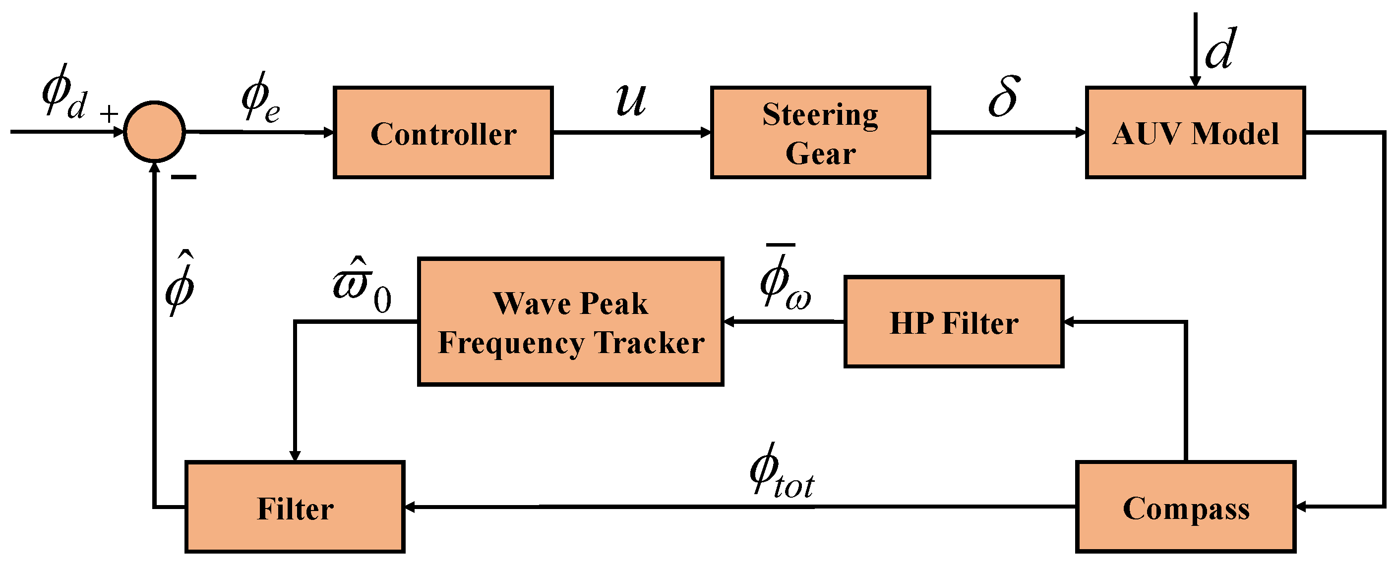
The heading control system of the AUV for producing the heading signal for the identification of the wave peak frequency is presented in Figure 2. The AUV heading signal ${\varphi }_{tot}$ is measured with an electronic compass and filtered by a high-pass filter. By using the filtered signal ${\overline{\varphi }}_{\omega }$, the wave peak frequency estimate ${\widehat{\varpi }}_0$ is obtained by the wave peak frequency tracker and then used to update the gains of the filter. $\widehat{\varphi }$ is the estimate of the LF components of the AUV heading signal, and $\widehat{r}$ is the estimate of the heading angle velocity. u is the rudder command, $\delta$ is the current rudder angle, and d is the wave disturbance.

4.1. Nomoto Model

In the current study, the Nomoto model is extensively employed for the heading control of an AUV when the AUV sails horizontally near the ocean surface or in shallow-water areas. The Nomoto model of an AUV can be represented as the following second-order system:

$$\begin{array}{cc}\hfill \dot{\varphi }& =r,\hfill \end{array}$$

(35)

$$\begin{array}{cc}\hfill \dot{r}& =-\frac{1}{T}r+\frac{K}{T}\delta ,\hfill \end{array}$$

(36)

where T and K are the model coefficients describing the motion characteristics of the ship, and $\delta$ is the rudder angle.

4.2. Back-Stepping Controller Design

To guarantee the real heading $\varphi$ of the AUV tracking the reference heading ${\varphi }_d$, the following back-stepping control design procedure is derived.

Define the heading angle error surface vector $z_1$ and heading angle rate error surface vector $z_2$ as

$$\begin{array}{cc}\hfill z_1& :=\varphi -{\varphi }_d,\hfill \end{array}$$

(37)

$$\begin{array}{cc}\hfill z_2& :=r-\chi ,\hfill \end{array}$$

(38)

where $\chi$ is a virtual controller to be designed later.

Step 1: Differentiating (37) with respect to time and using (38), we have

$$\begin{array}{cc}\hfill {\dot{z}}_1=& \dot{\varphi }-{\dot{\varphi }}_d\hfill \\ \hfill =& z_2+\chi -{\dot{\varphi }}_d.\hfill \end{array}$$

(39)

The virtual controller that is used to ensure the stability of the system (39) at $z_2=0$ can be designed as

$$\begin{array}{cc}\hfill \chi & :=-c_1{z}_1+{\dot{\varphi }}_d,\hfill \end{array}$$

(40)

where $c_1>0$ is a design parameter.

Substituting the controller (40) into (39), we have

$$\begin{array}{c}\hfill {\dot{z}}_1=z_2-c_1{z}_1.\end{array}$$

(41)

Step 2: Differentiating (38) with respect to time and combining it with (36) and (40), we have

$$\begin{array}{cc}\hfill {\dot{z}}_2=& \dot{r}-\dot{\chi }\hfill \\ \hfill =& -\frac{1}{T}r+\frac{K}{T}\delta +c_1{\dot{z}}_1-{\ddot{\varphi }}_d.\hfill \end{array}$$

(42)

The control law can be designed as

$$\begin{array}{cc}\hfill \delta & =\frac{T}{K}(\frac{1}{T}r-c_1{\dot{z}}_1+{\ddot{\varphi }}_d-z_1-c_2{z}_2),\hfill \end{array}$$

(43)

where $c_2>0$ is a design parameter.

Substituting the controller (43) into (42), we have

$$\begin{array}{c}\hfill {\dot{z}}_2=-z_1-c_2{z}_2.\end{array}$$

(44)

Step 3: We define a Lyapunov function candidate as

$$\begin{array}{c}\hfill V(z_1,z_2):=\frac{1}{2}{z}_1^2+\frac{1}{2}{z}_2^2.\end{array}$$

(45)

Differentiating the Lyapunov function with respect to time, we have

$$\begin{array}{c}\hfill \begin{array}{cc}\hfill \dot{V}(z_1,z_2)& =z_1{\dot{z}}_1+z_2{\dot{z}}_2\hfill \\ \hfill & =z_1(z_2+\chi -{\dot{\varphi }}_d)+z_2{\dot{z}}_2\hfill \\ \hfill & =z_1{z}_2-c_1{z}_1^2+z_2(-z_1-c_2{z}_2)\hfill \\ \hfill & =-c_1{z}_1^2-c_2{z}_2^2\hfill \\ \hfill & \le 0.\hfill \end{array}\end{array}$$

(46)

According to the Lyapunov stability theorem, the tracking errors $z_1$ and $z_2$ can converge to zero, and the closed-loop system is globally asymptotically stable.

4.3. Observer Design

Generally, a model-based observer often includes a disturbance model, where the goal is to estimate the forces of waves, winds, and ocean currents by treating them as colored noise. Hence, the observer design model is given by:

$$\begin{array}{c}\hfill \begin{array}{cc}\hfill {\dot{\zeta }}_{\varpi }& ={\varphi }_{\varpi },\hfill \\ \hfill {\dot{\varphi }}_{\varpi }& =-{\varpi }_0^2{\zeta }_{\varpi }-2\lambda {\varpi }_0{\zeta }_{\varpi }+w_1,\hfill \\ \hfill \dot{\varphi }& =r,\hfill \\ \hfill \dot{r}& =-\frac{1}{T}r+\frac{K}{T}\delta +w_r,\hfill \\ \hfill y& =\varphi +{\varphi }_{\varpi }+w_n,\hfill \end{array}\end{array}$$

(47)

where ${\zeta }_{\varpi }$ denotes the wave state, and $w_1,w_r$, and $w_n$ denote the white noises. To facilitate the observer design, the observer design model (47) can be written in a state-space form:

$$\begin{array}{cc}\hfill \dot{\mathit{x}}& =\mathit{A}\mathit{x}+\mathit{B}u+\mathit{E}\mathit{w},\hfill \end{array}$$

(48)

$$\begin{array}{cc}\hfill y& ={\mathit{h}}^T\mathit{x}+w_n,\hfill \end{array}$$

(49)

where

$$\begin{array}{cc}\hfill \mathit{x}& :={[{\zeta }_{\varpi },{\varphi }_{\varpi },\varphi ,r]}^T,\hfill \\ \hfill u& :=\delta ,\hfill \\ \hfill w& :={[w_1,w_r]}^T,\hfill \end{array}$$

$$\mathit{A}:=\left[\begin{array}{cccc}0& 1& 0& 0\\ -{\varpi }_0^2& 2\lambda {\varpi }_0^2& 0& 0\\ 0& 0& 0& 1\\ 0& 0& 0& -\frac{1}{T}\end{array}\right],\mathit{B}:=\left[\begin{array}{c}0\\ 0\\ 0\\ \frac{K}{T}\end{array}\right],$$

$$\mathit{E}:=\left[\begin{array}{cc}0& 0\\ 1& 0\\ 0& 0\\ 0& 1\end{array}\right],{\mathit{h}}^T:=\left[\begin{array}{cccc}0& 1& 1& 0\end{array}\right].$$

Then, we can obtain the observer of the ship heading system by neglecting the Gaussian white noise as follows:

$$\begin{array}{cc}\hfill \dot{\widehat{\mathit{x}}}& =\mathit{A}\widehat{\mathit{x}}+\mathit{B}u+{\mathit{k}}^T(y-\widehat{y}),\hfill \end{array}$$

(50)

$$\begin{array}{cc}\hfill \widehat{y}& ={\mathit{h}}^T\widehat{\mathit{x}},\hfill \end{array}$$

(51)

where $\widehat{\mathit{x}}$ and $\widehat{y}$ are the state vector and output of the observer, respectively, and ${\mathit{k}}^T$ is the observer gain vector, which can be selected as:

$$\begin{array}{c}\hfill \mathit{k}:=\left[\begin{array}{c}{K}_1\\ K_2\\ K_3\\ K_4\end{array}\right]=\left[\begin{array}{c}-2{\varpi }_0(1-\lambda )/{\varpi }_c\\ 2{\varpi }_0(1-\lambda )\\ {\varpi }_c\\ K_4\end{array}\right],\end{array}$$

(52)

where ${\varpi }_c$ is the cut-off frequency of the wave filter, and its value should be larger than the wave peak frequency ${\varpi }_0$. From this equation, we can see that the observer gain vector can be updated in real time by the identified wave peak frequency.

5. Simulation Results and Analysis

In this section, we selected the kinematic and kinetic models of a WL-3 AUV to carry out a closed-loop simulation experiment. The following simulation results show the performance of the wave peak frequency tracker. The parameters of the Nomoto model were set to $K=0.194$ and $T=0.695$ [50], and the reference velocity and heading angle were set to $2kn$ and ${30}^{\circ }$, respectively. The controller design parameters were set to $c_1=0.02$ and $c_2=10$. The relative damping ratio was set to $\xi =0.1$, the filter cut-off frequency ${\varpi }_c$ was chosen to be $1.1{\varpi }_0$, and $K_4$ was set to $0.01$. In order to be closer to the real situation, the rudder constraint was set to $\pm {24}^{\circ }$ according to the physical properties of the WL-3 AUV.

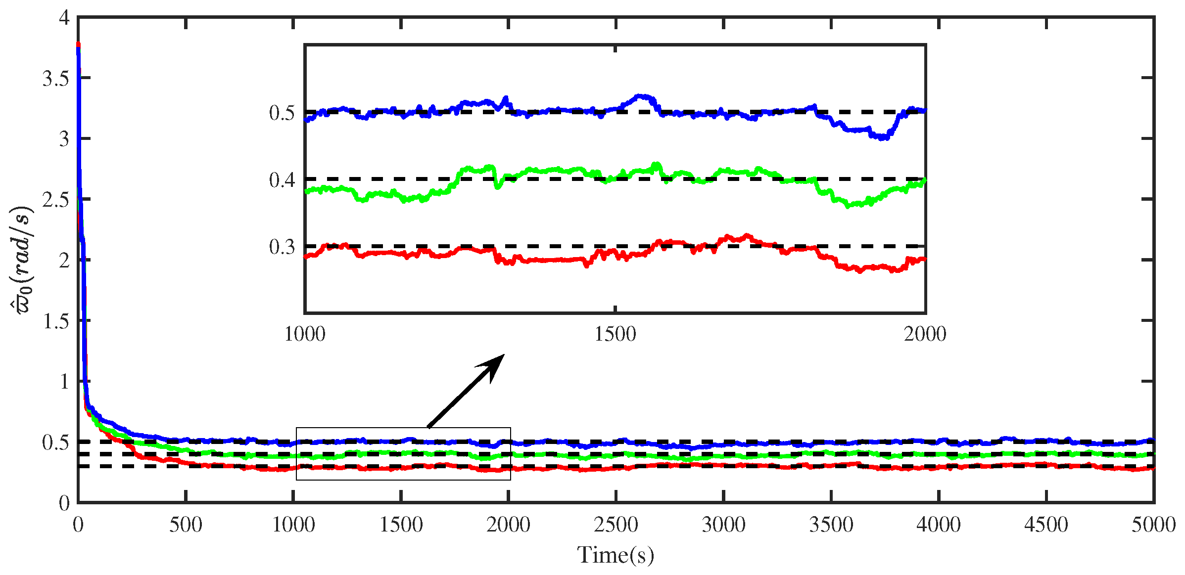
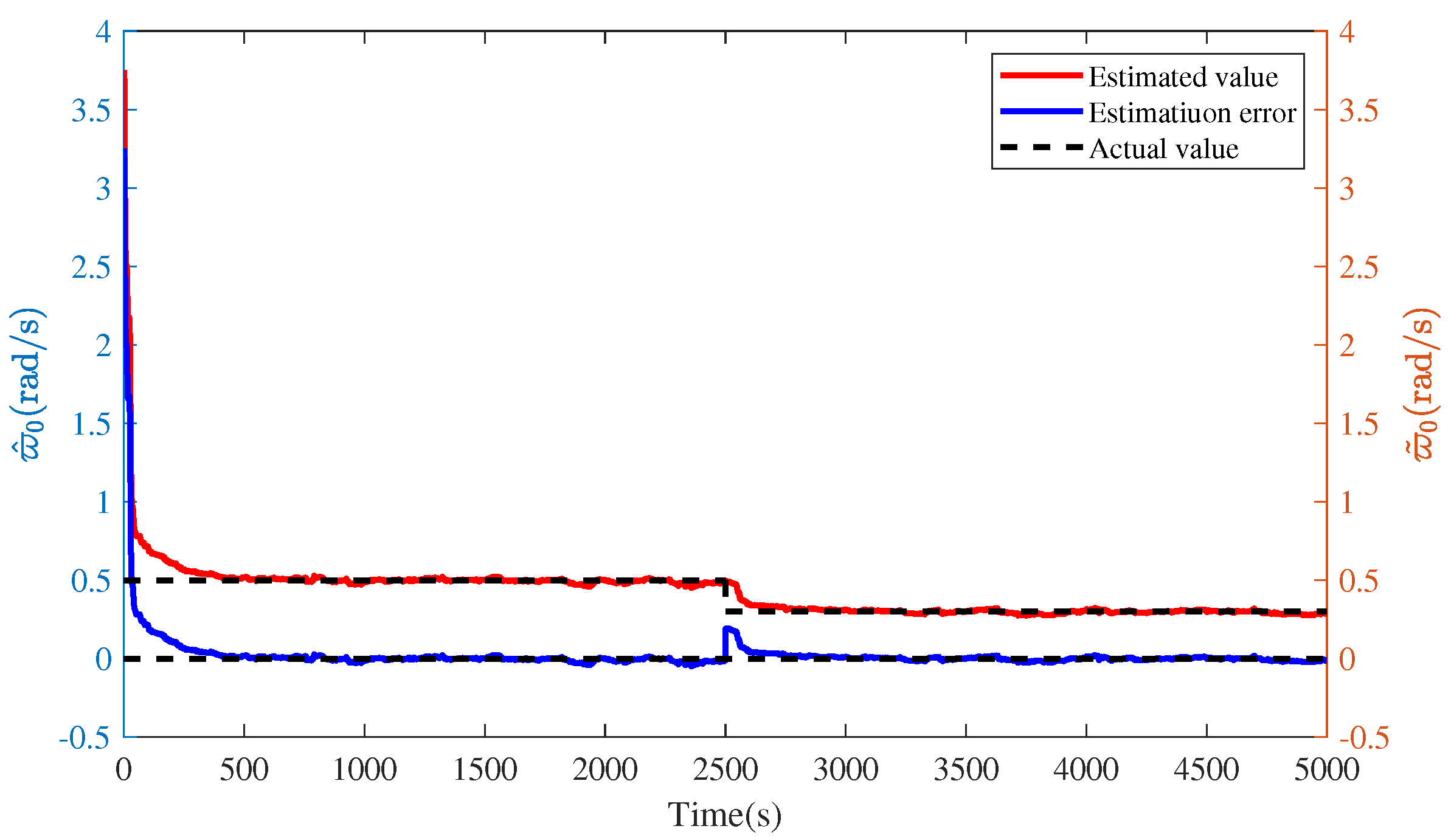
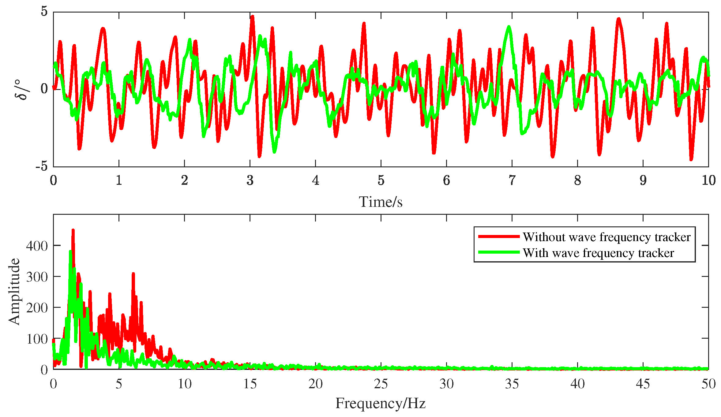
The simulation results for the proposed method are presented in Figure 3, Figure 4, Figure 5, Figure 6, Figure 7 and Figure 8. It can be seen from Figure 3 that the proposed RELS algorithm can estimate different wave peak frequencies under the same initial conditions. Furthermore, to evaluate the on-line identification ability of the proposed wave peak frequency tracker, the real wave peak frequency was set by changing $0.5$ to $0.3$ (rad/s). As seen in Figure 4, the wave peak frequency can be estimated accurately, and the estimation error curve is reasonable. Quantitative analyses of the wave peak frequency identification are listed in

Table 1. The estimates and estimation accuracy of the wave peak frequency when varying from ${\varpi }_0=0.5$ to ${\varpi }_0=0.3$ (rad/s) with the RELS algorithm.

t	${\widehat{\mathit{\varpi }}}_0$	$\mathit{\eta }$
100	0.71362	57.27539
200	0.60905	78.19031
500	0.51826	96.34836
1000	0.48592	97.18349
1500	0.50419	99.16230
2500	0.49000	98.00060
2600	0.35072	83.09367
2700	0.33395	88.68271
3000	0.31190	96.03276
3500	0.30010	99.96686
4000	0.30645	97.84896
4500	0.30126	99.57898
5000	0.28592	97.89700

. The wave peak frequency estimates ${\widehat{\varpi }}_0$ and the estimation accuracy $\eta$ are given, where $\eta =(1-\frac{{\widehat{\varpi }}_0-{\varpi }_0}{{\varpi }_0})\times 100\%$. It turns out that the proposed wave peak frequency tracking method is effective.

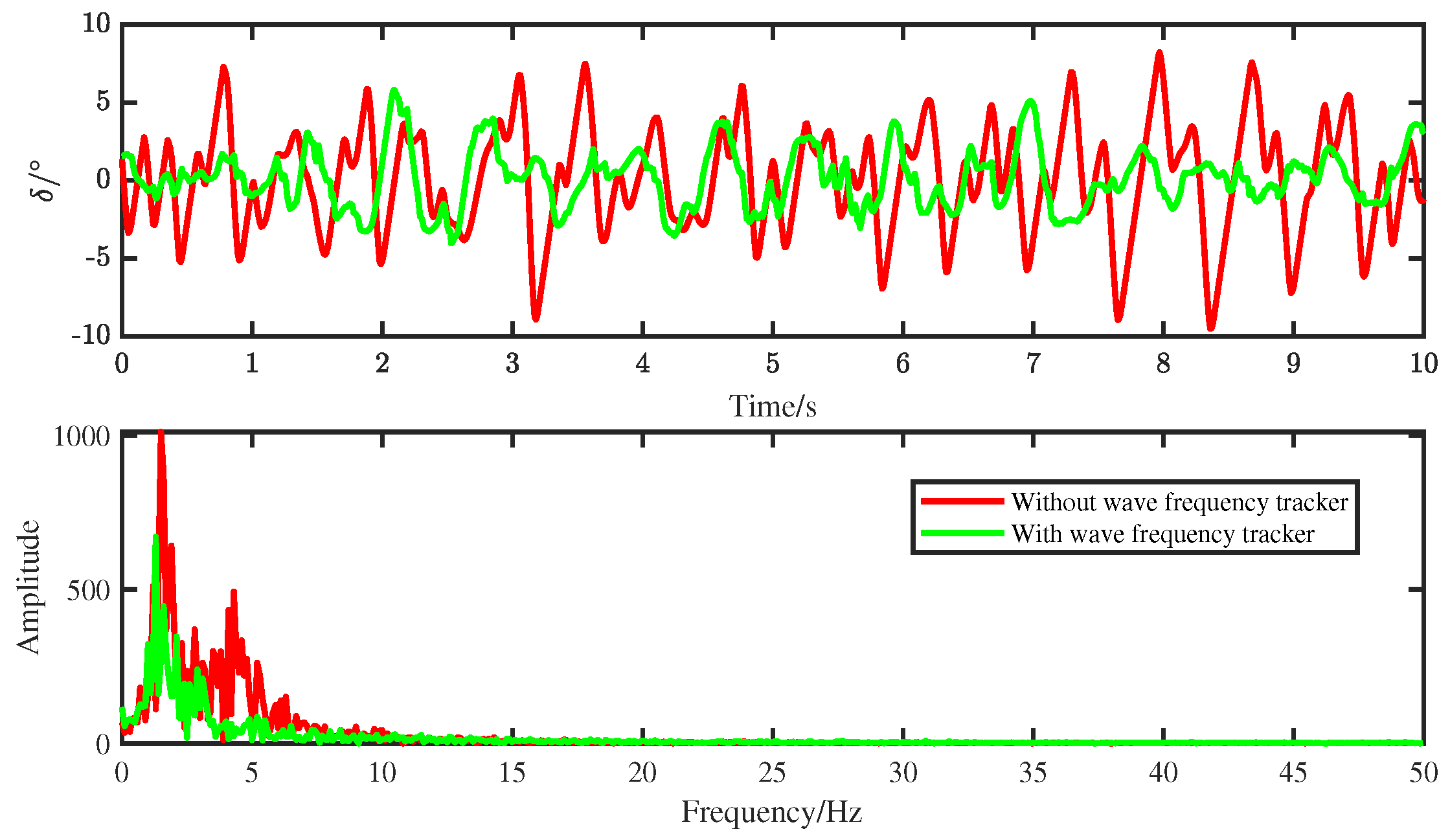
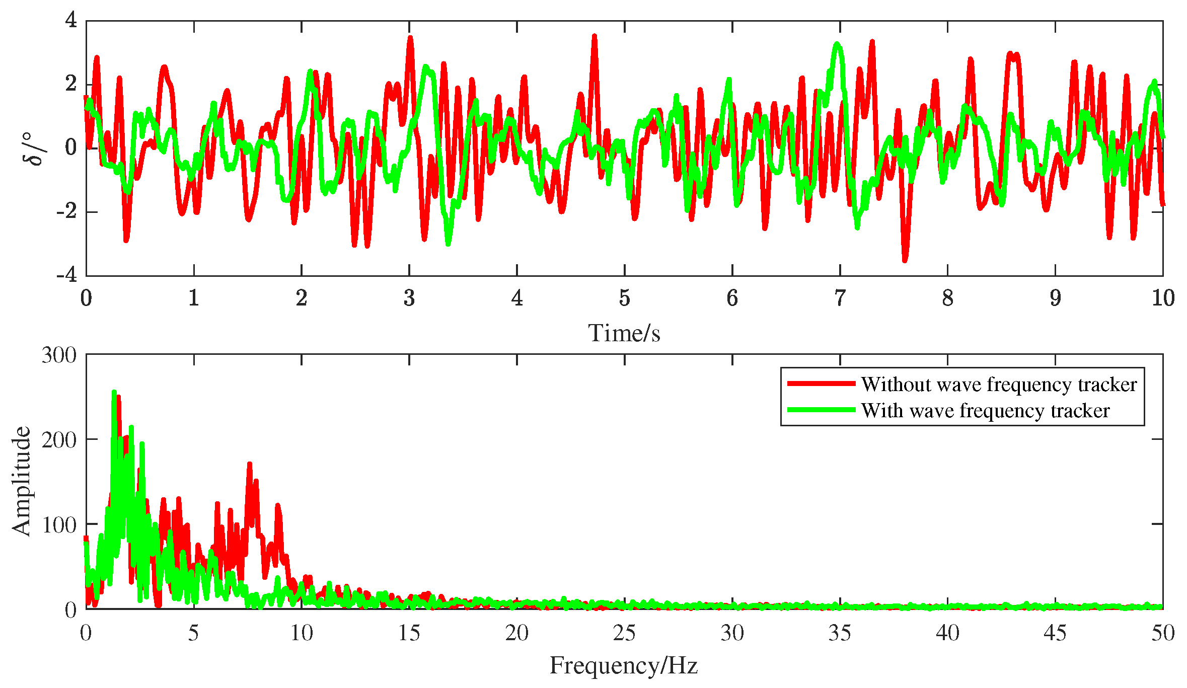
In order to verify the ability to reduce the invalid steering based on the wave peak frequency tracker, we set the unknown real wave peak frequency to ${\varpi }_0=0.3$ (rad/s), and the initial wave peak frequency ${\widehat{\varpi }}_0$ was supposed to be 1 (rad/s). As a contrast, the observer based on the wave frequency tracker was activated at 2500 (s). The rudder angle curve is plotted in Figure 5. To more intuitively illustrate the effectiveness of the proposed observer based on the wave peak frequency tracker, we chose two stable intervals, [1000 (s), 2000 (s)] and [3500 (s), 4500 (s)], to analyze the amplitude and frequency variations of the rudder angle. The amplitude–frequency map (the sampling frequency was selected as 100 (Hz)) is used to compare the variations in the frequency and amplitude of the rudder angle, as seen in Figure 6. It was implied that both the frequency and amplitude of the rudder angle were significantly reduced by using the observer based on the wave peak frequency tracker. Figure 7 and Figure 8 are amplitude–frequency maps at ${\varpi }_0=0.4$ and ${\varpi }_0=0.5$ (rad/s), respectively. The same conclusion was made as that for ${\varpi }_0=0.3$ (rad/s).

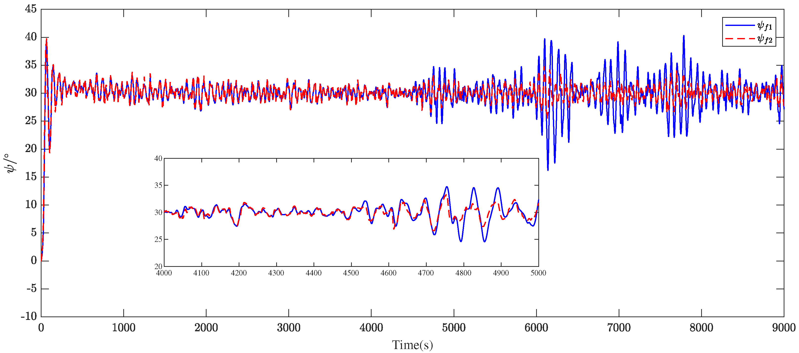
In order to further evaluate the superiority of the filter based on the wave peak frequency tracker, the heading angle under the filter with a constant wave peak frequency ${\psi }_{f1}$ and the heading angle under the filter with the wave peak frequency tracker ${\psi }_{f2}$ are given in Figure 9. It can be seen that the filter based on the wave peak frequency tracker had a superior performance to that of the filter with a constant wave peak frequency.

6. Conclusions

Based on the idea of auxiliary model identification, this paper presents an auxiliary-model-based recursive extended least-squares identification algorithm for identifying the wave peak frequency. In order to obtain the identification model, the wave disturbance state-space model was converted into an input–output expression by eliminating the intermediate variable. The heading control system of an AUV using the wave peak frequency tracker was established to evaluate the effectiveness of the proposed method. The simulation results demonstrate that the proposed algorithm can accurately track the wave peak frequency, and the frequency and amplitude of the rudder angle are significantly reduced by using the observer based on the wave peak frequency tracker. The accuracy of the estimation of the wave peak frequency is important for the wave filter. In order to enhance the parameter estimation accuracy, some other excellent methods, such as data-filtering-based algorithms and maximum-likelihood-based algorithms, can be combined to present new algorithms. In the future, we will integrate a data-filtering technique and the principle of maximum likelihood identification to study new algorithms in order to enhance the accuracy of the estimation of the wave peak frequency.

References

1. Khodayari, M.H.; Balochian, S. Modeling and control of autonomous underwater vehicle (AUV) in heading and depth attitude via self-adaptive fuzzy PID controller. J. Mar. Sci. Technol. 2015, 20, 559–578. [Google Scholar] [CrossRef]
2. Garcia-Garcia, D.; Valeriano-Medina, Y.; Hernández, L.; Martínez, A.; Martínez-Espinosa, Y. Wave disturbance compensation for AUV diving control in shallow water environment. J. Appl. Res. Technol. 2019, 17, 326–337. [Google Scholar]
3. Dantas, J.L.D.; de Barros, E.A.; da Cruz, J.J. AUV control in the diving plane subject to waves. IFAC Proc. Vol. 2012, 45, 319–324. [Google Scholar] [CrossRef]
4. Fossen, T.I. Guidance and Control of Ocean Vehicles; Wiley: New York, NY, USA, 1994. [Google Scholar]
5. Fossen, T.I. Handbook of Marine Craft Hydrodynamics and Motion Control; John Wiley & Sons: Noida, India, 2011. [Google Scholar]
6. Sakai, M.; Umeda, N.; Maki, A. Encounter frequency effect on the simplified design criteria against parametric roll. Ocean Eng. 2019, 182, 21–27. [Google Scholar] [CrossRef]
7. Værnø, S.A.; Skjetne, R.; Kjerstad, ø.K.; Calabrò, V. Comparison of control design models and observers for dynamic positioning of surface vessels. Control Eng. Pract. 2019, 85, 235–245. [Google Scholar] [CrossRef]
8. Zhang, X.; Han, X.; Guan, W.; Zhang, G. Improvement of integrator backstepping control for ships with concise robust control and nonlinear decoration. Ocean Eng. 2019, 189, 106349. [Google Scholar] [CrossRef]
9. Guan, W.; Cao, W.; Sun, J.; Su, Z. Steering controller design for smart autonomous surface vessel based on CSF L2 gain robust strategy. IEEE Access 2019, 7, 109982–109989. [Google Scholar] [CrossRef]
10. Ding, F. System Identification—New Theory and Methods; Science: Beijing, China, 2013. [Google Scholar]
11. Xu, L. Parameter estimation algorithms for dynamical response signals based on the multi-innovation theory and the hierarchical principle. IET Signal Process. 2017, 11, 228–237. [Google Scholar] [CrossRef]
12. Ma, F.; Yin, Y.; Li, M. Start-up process modelling of sediment microbial fuel cells based on data driven. Math. Probl. Eng. 2019, 2019, 7403732. [Google Scholar] [CrossRef]
13. Van Wingerden, J.; Verhaegen, M. Subspace identification of bilinear and LPV systems for open-and closed-loop data. Automatica 2009, 45, 372–381. [Google Scholar] [CrossRef]
14. Sun, Z.; Zhang, D.; Meng, Q.; Chen, C. Feedback stabilisation of time-delay nonlinear systems with continuous time-varying output function. Int. J. Syst. Sci. 2019, 50, 244–255. [Google Scholar] [CrossRef]
15. Li, M.; Liu, X. The filtering-based maximum likelihood iterative estimation algorithms for a special class of nonlinear systems with autoregressive moving average noise using the hierarchical identification principle. Int. J. Adapt. Control Signal Process. 2019, 33, 1189–1211. [Google Scholar] [CrossRef]
16. Wang, Y.; Ding, F.; Wu, M. Recursive parameter estimation algorithm for multivariate output-error systems. J. Frankl. Inst. 2018, 355, 5163–5181. [Google Scholar] [CrossRef]
17. Wang, D. Input–output data filtering based recursive least squares identification for CARARMA systems. Digit. Signal Process. 2010, 20, 991–999. [Google Scholar] [CrossRef]
18. Xiao, Y.; Yue, N. Parameter estimation for nonlinear dynamical adjustment models. Math. Comput. Model. 2011, 54, 1561–1568. [Google Scholar] [CrossRef]
19. Ding, F.; Liu, X.; Chu, J. Gradient-based and least-squares-based iterative algorithms for Hammerstein systems using the hierarchical identification principle. IET Control Theory Appl. 2013, 7, 176–184. [Google Scholar] [CrossRef]
20. Ding, F.; Liu, P.X.; Liu, G. Gradient based and least-squares based iterative identification methods for OE and OEMA systems. Digit. Signal Process. 2010, 20, 664–677. [Google Scholar] [CrossRef]
21. Ding, F. Two-stage least squares based iterative estimation algorithm for CARARMA system modeling. Appl. Math. Model. 2013, 37, 4798–4808. [Google Scholar] [CrossRef]
22. Ding, F. Decomposition based fast least squares algorithm for output error systems. Signal Process. 2013, 93, 1235–1242. [Google Scholar] [CrossRef]
23. Ding, F.; Chen, H.; Xu, L.; Dai, J.; Li, Q.; Hayat, T. A hierarchical least squares identification algorithm for Hammerstein nonlinear systems using the key term separation. J. Frankl. Inst. 2018, 355, 3737–3752. [Google Scholar] [CrossRef]
24. Ji, Y.; Jiang, X.; Wan, L. Hierarchical least squares parameter estimation algorithm for two-input Hammerstein finite impulse response systems. J. Frankl. Inst. 2020, 357, 5019–5032. [Google Scholar] [CrossRef]
25. Xu, L.; Xiong, W.; Alsaedi, A.; Hayat, T. Hierarchical parameter estimation for the frequency response based on the dynamical window data. Int. J. Control Autom. Syst. 2018, 16, 1756–1764. [Google Scholar] [CrossRef]
26. Wang, D.; Zhang, W. Improved least squares identification algorithm for multivariable Hammerstein systems. J. Frankl. Inst. 2015, 352, 5292–5307. [Google Scholar] [CrossRef]
27. Chen, H.; Ding, F.; Xiao, Y. Decomposition-based least squares parameter estimation algorithm for input nonlinear systems using the key term separation technique. Nonlinear Dyn. 2015, 79, 2027–2035. [Google Scholar] [CrossRef]
28. Ji, Y.; Kang, Z. Three-stage forgetting factor stochastic gradient parameter estimation methods for a class of nonlinear systems. Int. J. Robust Nonlinear Control 2021, 31, 971–987. [Google Scholar] [CrossRef]
29. Xu, L. The damping iterative parameter identification method for dynamical systems based on the sine signal measurement. Signal Process. 2016, 120, 660–667. [Google Scholar] [CrossRef]
30. Xu, L. Separable multi-innovation stochastic gradient estimation algorithm for the nonlinear dynamic responses of systems. Int. J. Adapt. Control Signal. 2020, 34, 937–954. [Google Scholar] [CrossRef]
31. Wang, L.; He, Y. Recursive least squares parameter estimation algorithms for a class of nonlinear stochastic systems with colored noise based on the auxiliary model and data filtering. IEEE Access 2019, 7, 181295–181304. [Google Scholar] [CrossRef]
32. Guo, C.; Wang, L.; Deng, F. The auxiliary model based hierarchical estimation algorithms for bilinear stochastic systems with colored noises. Int. J. Control Autom. Syst. 2020, 18, 650–660. [Google Scholar] [CrossRef]
33. Wang, C.; Tang, T. Recursive least squares estimation algorithm applied to a class of linear-in-parameters output error moving average systems. Appl. Math. Lett. 2014, 29, 36–41. [Google Scholar] [CrossRef]
34. Du, J.; Hu, X.; Krstić, M.; Sun, Y. Dynamic positioning of ships with unknown parameters and disturbances. Control Eng. Pract. 2018, 76, 22–30. [Google Scholar] [CrossRef]
35. Deng, F.; Wang, L.; Jiao, D. Adaptive observer based backstepping controller design for dynamic ship positioning. China Ocean Eng. 2017, 31, 639–645. [Google Scholar] [CrossRef]
36. Torsetnes, G.; Jouffroy, J.; Fossen, T.I. Nonlinear dynamic positioning of ships with gain-scheduled wave filtering. In Proceedings of the 2004 43rd IEEE Conference on Decision and Control (CDC) (IEEE Cat. No.04CH37601), Nassau, Bahamas, 14–17 December 2004; pp. 5340–5347. [Google Scholar]
37. Wang, X.; Xu, H. Robust autopilot with wave filter for ship steering. J. Mar. Sci. Appl. 2006, 5, 24–29. [Google Scholar]
38. Hassani, V.; Pascoal, A.M.; Aguiar, A.P.; Athans, M. A multiple model adaptive wave filter for dynamic ship positioning. IFAC Proc. Vol. 2010, 43, 120–125. [Google Scholar] [CrossRef] [Green Version]
39. Lauvdal, T.; Fossen, T.I. Robust adaptive ship autopilot with wave filter and integral action. Int. J. Adapt. Control Signal Process. 1998, 12, 605–622. [Google Scholar] [CrossRef]
40. Fossen, T.I. Marine Control Systems: Guidance, Navigation and Control of Ships, Rigs and Underwater Vehicles; Marine Cybernetics: Trondheim, Norway, 2002. [Google Scholar]
41. Bryne, T.H.; Fossen, T.I.; Johansen, T.A. Design of inertial navigation systems for marine craft with adaptive wave filtering aided by triple-redundant sensor packages. Int. J. Adapt. Control Signal Process. 2017, 31, 522–544. [Google Scholar] [CrossRef] [Green Version]
42. Hassani, V.; Pascoal, A.M.; Sørensen, A.J. A novel methodology for adaptive Wave Filtering of marine vessels: Theory and experiments. In Proceedings of the 52nd IEEE Conference on Decision and Control, Firenze, Italy, 10–13 December 2013; pp. 6162–6167. [Google Scholar]
43. Gu, Y.; Zhu, Q.; Nouri, H. Bias compensation-based parameter and state estimation for a class of time-delay non-linear state-space models. IET Control Theory Appl. 2020, 14, 2176–2185. [Google Scholar] [CrossRef]
44. Gu, Y.; Zhu, Q.; Li, C.; Zhu, P.; Nouri, H. State filtering and parameter estimation for two-input two-output systems with time delay. IET Control Theory Appl. 2021, 15, 2053–2066. [Google Scholar] [CrossRef]
45. Xu, L.; Chen, F. Hierarchical recursive signal modeling for multifrequency signals based on discrete measured data. Int. J. Adapt. Control Signal. 2021, 35, 676–693. [Google Scholar] [CrossRef]
46. Ji, Y.; Zhang, C.; Kang, Z.; Yu, T. Parameter estimation for block-oriented nonlinear systems using the key term separation. Int. J. Robust Nonlinear Control 2020, 30, 3727–3752. [Google Scholar] [CrossRef]
47. Wang, L.; Ji, Y.; Wan, L.; Bu, N. Hierarchical recursive generalized extended least squares estimation algorithms for a class of nonlinear stochastic systems with colored noise. J. Frankl. Inst. 2019, 356, 10102–10122. [Google Scholar] [CrossRef]
48. Wang, L.; Ji, Y.; Yang, H.; Xu, L. Decomposition-based multiinnovation gradient identification algorithms for a special bilinear system based on its input-output representation. Int. J. Robust Nonlinear Control 2020, 30, 3607–3623. [Google Scholar] [CrossRef]
49. Xu, L.; Song, G. A recursive parameter estimation algorithm for modeling signals with multi-frequencies. Circuits Syst. Signal Process. 2020, 39, 4198–4224. [Google Scholar] [CrossRef]
50. An, L.; Li, Y.; Jiang, Y.; Li, Y.; Cao, J.; He, J. Soft-switching proximate time optimal heading control for underactuated autonomous underwater vehicle. IEEE Access 2019, 7, 143233–143249. [Google Scholar]
Figure 1. The flowchart of the RELS algorithm for computing θ ^ ( t ) .
Sustainability 14 15357 g001
Figure 2. The heading control system of the AUV.
Sustainability 14 15357 g002
Figure 3. Identification for different wave peak frequencies.
Sustainability 14 15357 g003
Figure 4. The wave peak frequency estimate ϖ ^ 0 and estimation error ϖ ˜ 0 .
Sustainability 14 15357 g004
Figure 5. The rudder angle at ϖ 0 = 0.3 (rad/s).
Sustainability 14 15357 g005
Figure 6. The amplitude and frequency of the rudder angle at ϖ 0 = 0.3 (rad/s).
Sustainability 14 15357 g006
Figure 7. The amplitude and frequency of the rudder angle at ϖ 0 = 0.4 (rad/s).
Sustainability 14 15357 g007
Figure 8. The amplitude and frequency of the rudder angle at ϖ 0 = 0.5 (rad/s).
Sustainability 14 15357 g008
Figure 9. Comparison of the heading angle under the wave peak frequency from 0.5 to 0.3 rad/s.
Sustainability 14 15357 g009