Article

Deep-Reinforcement-Learning-Based Active Disturbance Rejection Control for Lateral Path Following of Parafoil System

1
College of Artificial Intelligence, Nankai University, Tianjin 300350, China
2
Silo AI, 00100 Helsinki, Finland
3
Key Laboratory of Intelligent Robotics of Tianjin, Nankai University, Tianjin 300350, China
*
Authors to whom correspondence should be addressed.
Sustainability 2023, 15(1), 435; https://doi.org/10.3390/su15010435
Submission received: 9 November 2022 / Revised: 19 December 2022 / Accepted: 22 December 2022 / Published: 27 December 2022

Abstract

:
The path-following control of the parafoil system is essential for executing missions, such as accurate homing and delivery. In this paper, the lateral path-following control of the parafoil system is studied. First, considering the relative motion between the parafoil canopy and the payload, an eight-degree-of-freedom (DOF) model of the parafoil system is constructed. Then, a guidance law containing the position deviation and heading angle deviation is proposed. Moreover, a linear active disturbance rejection controller (LADRC) is designed based on the guidance law to allow the parafoil system to track the desired path under internal unmodeled dynamics or external environmental disturbances. For the adaptive tuning of the controller parameters, a deep Q-network (DQN) is applied to the LADRC-based path-following control system, and the controller parameters can be adjusted in real time according to the system’s states. Finally, the effectiveness of the proposed method is applied to a parafoil system following circular and straight paths in an environment with wind disturbances. The simulation results show that the proposed method is an effective means to realize the lateral path-following control of the parafoil system, and it can also promote the development of intelligent controllers.

1. Introduction

A parafoil system is a unique aircraft consisting of a parafoil canopy, connecting rope, and payload. With its excellent gliding ability and payload characteristics, the parafoil system is currently widely used in aerospace, military, and civil fields. However, the parafoil system applies a flexible canopy to provide the lift force, so it has complicated dynamic characteristics and strong nonlinearity [1]. During flight, the parafoil can be affected by unpredictable wind disturbances. Therefore, determining how to overcome these disturbances and accurately control the parafoil system to follow the desired path is the key to completing missions.
Limited by actual flight tests, which require considerable preparation work and are time-consuming and expensive, a mathematical model is a prerequisite for analyzing the motion characteristics of the parafoil system. To the best of our knowledge, according to the division of the DOFs, the current existing modeling methods include longitudinal four-DOF [2], six-DOF [3,4], eight-DOF [5,6], and nine-DOF [7] models. These models were all obtained through force analysis of the parafoil system. In this paper, considering the relative pitch and yaw motions between the parafoil canopy and the payload, we constructed an eight-DOF model based on a six-DOF model [5].
There have been some research results for the path-following control of the parafoil system. For example, Tao et al. [8] applied a generalized predictive control (GPC)-based method for a parafoil system to follow the designed path for a better control effect, where the guidance law was based on a combination of tracking errors. Zhao et al. [9] introduced a model-free adaptive control method based on iterative feedback tuning (IFT-MFAC) method for parafoil systems, where only the input/output data are needed during the construction. Guo et al. [10] proposed an improved adaptive path-following guidance law to reduce the effect of time-varying wind disturbances, where the convergence rate was improved by replacing the function. Li et al. [11] designed three proportional–integral–derivative (PID) controllers for the lateral motion, longitudinal motion, and velocity on the basis of the motion characteristics of the parafoil system, which overcame the limitations of the traditional guidance-based tracking strategy. As for actual airdrop scenarios, the PID controller still occupies a dominant position, but the PID controller cannot achieve high tracking accuracy, especially under the disturbances of a complex environment. Tao et al. [12,13] used linear active disturbance rejection control (LADRC) to realize the accurate trajectory tracking of the parafoil system. LADRC is currently the most widely used control strategy in practice besides PID; however, the adjustment of the LADRC parameters remains a challenging problem to be studied.
Active disturbance rejection control (ADRC) [14] was first proposed by Han [15], which combines the state observer in modern theory with the error-based ideas in PID. Specifically, ADRC uses an extended state observer (ESO) to observe the unknown disturbances in the system and uses a state error feedback (SEF) control law to eliminate the disturbance. With model-free characteristics and good control effects, ADRC has attracted the attention of many scholars. Gao [16] developed LADRC through the linearization of the ESO and SEF, which significantly promoted the theoretical and engineering application research of ADRC. In terms of theory, Chen [17] and Wang [18] provided proof of the stability of LADRC. LADRC has demonstrated its control advantages in applications such as power system load frequency control (LFC) [19], heading angle control [20], path-following control [21,22], and an electromechanical servo system [23]. For example, Li et al. [24] proposed a guidance law based on a ship’s nonlinear combination of lateral error and heading angle error, and LADRC was used to estimate and eliminate the disturbances. However, this guidance law could only realize path tracking in the y-direction. Inspired by this result, this paper proposes a new guidance law.
Although the number of parameters that need to be adjusted in the LADRC controller has significantly been reduced compared to that in the ADRC, parameter optimization is still a non-negligible part of the controller design process. In most cases, researchers will manually adjust the controller parameters, which makes it challenging to achieve the system’s optimal performance. Therefore, various optimization algorithms have emerged continually. The robustness of heuristic algorithms that can optimize a set of fixed parameters, such as the particle swarm optimization (PSO) algorithm [25] and genetic algorithm (GA) [26], is somewhat limited. For algorithms that can achieve adaptive optimization, such as neural networks [27] and fuzzy control [28], these algorithms have difficulty achieving better results when encountering unknown emergencies.
Deep reinforcement learning (DRL) is a combination of reinforcement learning (RL) and neural networks that uses the computing power of neural networks and encompasses the decision-making ability of RL. With the intelligent characteristics of not relying on models and being able to make decisions autonomously, similar to the human brain, DRL is favored by many scholars. The deep Q-network (DQN) [29] is one of the most classical algorithms in DRL, and it overcomes the shortcomings of the Q table in Q-learning of RL whereby it is difficult to express all states. In other words, the DQN can handle systems with continuous states. The application of DQN in path-following control is mainly to make direct decisions in terms of the control variable. For example, Zhao et al. [30] used DQN to determine the rudder angle and propeller speed during the path tracking of an unmanned surface vessel (USV), which completely separated decision-making and control theory. At present, there are few studies on the application of RL in parafoil systems. Therefore, to promote the development of intelligent controllers in parafoil systems, this paper uses the DQN algorithm to optimize the parameters of the LADRC controller.
Inspired by the previous research, we proposed a DQN-optimized LADRC method for lateral path-following control of the parafoil system in this paper. The main contributions of this paper are summarized as follows:
  • A new guidance law for the lateral path-following control of the parafoil system is proposed.
  • Based on the guidance law, an LADRC controller is designed to overcome the influence of unknown disturbances during parafoil flight.
  • The DQN algorithm of RL is applied to obtain the real-time parameters of the controller based on the parafoil flight states.
The rest of the paper is organized as follows. The eight-DOF parafoil system model is established in Section 2. Section 3 introduces the guidance law and provides the corresponding design process of the LADRC-based path-following controller. Section 4 presents the design process of the DQN-optimized LADRC. The simulation results are given in Section 5, and Section 6 concludes this paper.

2. Dynamic Model of Parafoil System

In the six-DOF parafoil model, the parafoil canopy and payload are regarded as rigid connections, and the relative motion between the two is ignored. In order to describe the motion characteristics of the parafoil more accurately, an eight-DOF dynamic model is established in this paper. The slew, sway, yaw, heave, pitch, and roll motions of the parafoil canopy, and the relative pitch and relative yaw motion between the parafoil canopy and the payload are considered. In this way, we can better observe the attitude of the parafoil system during the movement. Three coordinate systems are established to facilitate parafoil system modeling: the ground coordinate system O d x d y d z d , the parafoil coordinate system O s x s y s z s , and the payload coordinate system O w x w y w z w , as shown in Figure 1.
Furthermore, since the actual model is very complex, in the process of building the model in this paper, the following three assumptions are adopted, and certain simplifications are made:
  • The mass center of the parafoil canopy coincides with the aerodynamic pressure center but does not coincide with the gravity center.
  • The lift of the payload is ignored and only the aerodynamic drag is considered.
  • The elastic deformation of the connecting ropes is ignored.

2.1. Motion Equation of Payload

In this paper, the payload is regarded as a rigid body subjected to aerodynamic forces, gravity, and the pulling force of the connecting rope. The force and moment balance equations of the payload are expressed as
P w t + W w × P w = F w a e r o + F w G + F w t H w t + W w × H w = M w a e r o + M w f + M w t ,
where P and H represent the momentum and angular momentum, defined below. The superscripts a e r o , G, t, and f represent the aerodynamic force, gravity, connecting rope tension, and friction, respectively. V w = u w , v w , w w T denotes the velocity vector, and W w = p w , q w , r w T denotes the angular velocity vector. The momentum and angular momentum are defined, respectively, as follows:
P w = m w V w H w = J w W w .
The tension and tension moment of the connecting rope are expressed as
F w t = F 1 + F 2 M w t = [ L w 1 L w 2 ] [ F w 1 T F w 2 T ] T ,
where F 1 and F 2 represent the tension at points c 1 and c 2 , respectively. L w 1 = l 2 0 1 0 1 0 0 0 0 0 , L w 2 = l 1 2 0 0 1 0 0 0 1 0 0 , and l 1 refers to the distance between the connection points c 1 and c 2 . l 2 is the distance between the O w of the payload coordinate system and the midpoint c 0 of the two connecting points.

2.2. Motion Equation of Parafoil Canopy

When the canopy is fully inflated and unfolded, the force on the canopy includes aerodynamic forces, gravity, and the pulling force of the connecting rope. The equations of the conservation of linear and angular momentum of the parafoil canopy are expressed, respectively, as
P s t + W s × P s = F s a e r o + F s G + F s t H s t + W s × H s + V s × P s = M s a e r o + M s G + M s f + M s t .
Similarly, the velocity vector V s = u s , v s , w s T and angular velocity vector W s = p s , q s , r s T are defined. It should be pointed out that the movement of the parafoil canopy in the air can be approximately regarded as the movement in an ideal fluid. Hence, the influence of the additional mass on the system needs to be considered. Therefore, the linear momentum and angular momentum of the parafoil canopy considering the additional mass are described as
P s H s = A a + A r V s W s ,
where A a denotes the inertia matrix of the additional mass, and A r represents the inertia matrix of the canopy’s real mass.
Similarly, in the parafoil coordinate system, there is an expression of the tension of the connecting rope relative to the moment of the parasol center of mass:
M s t = L s 1 T w s L s 2 T w s F w 1 T F w 2 T T ,
where T w s is defined below. L s 1 = l 3 0 1 0 1 0 0 0 0 0 , L s 2 = l 1 2 0 0 cos ψ r 0 0 sin ψ r cos ψ r sin ψ r 0 , and l 3 represents the distance between the O s of the payload coordinate system and c 0 .

2.3. Constraints of Velocity and Angular Velocity

As shown in Figure 1, the canopy and the payload are connected by ropes at two connection points, c 1 and c 2 , and then the midpoint c 0 of the two points can be regarded as the total connection point. At this point, there is the following velocity constraint:
V w + W w × L w c = V s + W s × L s c ,
where L w c and L s c represent the distance from the payload centroid to c 0 and the distance from the parafoil canopy centroid to c 0 , respectively. Differentiation of Equation (7) can yield the following formula:
V ˙ s L s c × W ˙ s T w s V ˙ w + T w s L w c × W ˙ w = T w s W w × V w + W w × L w c W s × V s + W s × L s c ,
where T w s is the conversion matrix from the payload coordinate system to the canopy coordinate system. T w s is expressed as follows:
T w s = cos θ r cos ψ r sin ψ r sin θ r cos ψ r cos θ r sin ψ r cos ψ r sin θ r sin ψ r sin θ r 0 cos θ r ,
where θ r and ψ r denote the relative pitch angle and relative yaw angle, respectively.
As for the relative rotation between the payload and the canopy, the following angular velocity constraint is satisfied:
W w = W s + τ s + κ w ,
where τ s = 0 , 0 , ψ ˙ r T , and κ w = 0 , θ ˙ r , 0 T . The derivative of Equation (10) is as follows:
T w s W ˙ w W ˙ s T w s κ ˙ w τ ˙ s = W s T w s W w × W s T w s κ w × τ s .
Define the state variable as x s = V w T , W w T , V s T , W s T , ψ ˙ r , θ ˙ r T . Then, by combining Equations (1)–(4), (8) and (11), the eight-DOF dynamic model of the parafoil can be expressed as follows:
x ˙ s = D 1 T , D 2 T , D 3 T , D 4 T T 1 E 1 T , E 2 T , E 3 T , E 4 T T .
Refer to [4] for a more detailed modeling process.
By denoting s i n θ as s θ and c o s θ as c θ , the following equation can be obtained:
x ˙ y ˙ z ˙ = c θ c ψ c θ s ψ s θ s ϕ s θ c ψ c ϕ s ψ s ϕ s θ s ψ + c ϕ c ψ s ϕ c θ c ϕ s θ c ψ + s ϕ s ψ c ϕ s θ s ψ s ϕ c ψ c ϕ c θ T V s ,
where ϕ , θ , and ψ are three Euler angles, i.e., the roll angle, pitch angle, and yaw angle, respectively. Based on Equations (12) and (13), the position of the parafoil can be obtained.
In this paper, the parafoil system is described by the dynamic and kinematic parameters. The dynamic parameters of the parafoil system are the parameters that describe the forces and moments in Equations (1) and (4), which are mainly used to express the relationship between the force of the parafoil system and its motion. The kinematic parameters of the parafoil system are the parameters describing the speed, Euler angles, and acceleration of the parafoil system in Equation (13), which reflects the variation of the position of the parafoil system with time. It is worth mentioning that during the movement of the parafoil, unmodeled dynamics and disturbances in the external environment will cause unpredictable effects. Therefore, the mismatch between theory and reality challenges the controller design.

3. Linear Active Disturbance Rejection Controller (LADRC)-Based Path-Following Control

As mentioned above, the direction of the parafoil system is manipulated by control ropes connecting two sides of the canopy. Specifically, the left control rope is pulled downward to realize a left turn and the right control rope is pulled down to realize a right turn. That is, by controlling the control ropes on both sides, the position and heading angle of the parafoil system are changed simultaneously to track the desired path. Overall, the control command produced by the control system will result in the increase in the force of one of the ropes. Moreover, in the actual control process, the control signal is usually transmitted to the rope in the form of a differential or pulse (1/0), which also brings difficulty to the control system.

3.1. Guidance Law

To achieve convergence of the parafoil position deviation and heading angle deviation to zero simultaneously, according to a guidance law designed in Reference [24], a new guidance law is established as follows:
g = g 0 tanh g 1 · Δ d + ψ ψ d ,
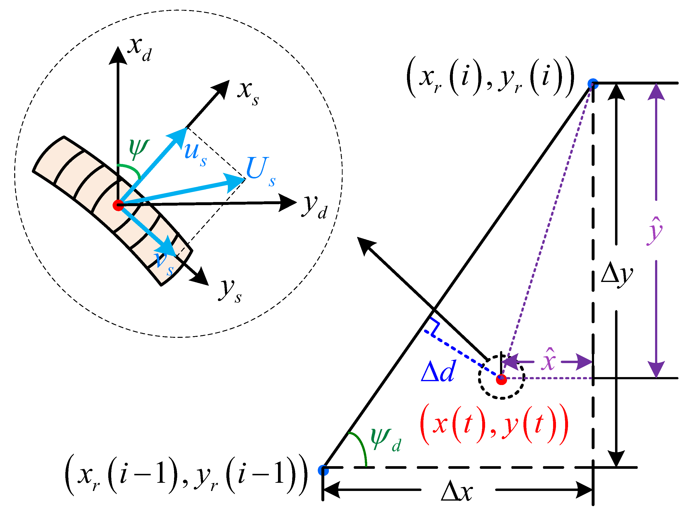
where g 0 and g 1 are adjustable parameters ( g 0 > 0 , g 1 > 0 ). ψ and ψ d represent the true value and the planned value of the parafoil’s heading angle (yaw angle), respectively. Δ d is the position tracking error, as shown in Figure 2, expressed as follows:
Δ d = x ^ Δ y y ^ Δ x Δ x 2 + Δ y 2 ψ d = a r c tan Δ y / Δ x .
As shown in Figure 2, the red point ( x ( t ) , y ( t ) ) represents the current position of the parafoil, and the blue points x r i 1 , y r i 1 and x r i , y r i are the two adjacent points in the desired path. Define
Δ x = x r i x r i 1 Δ y = y r i y r i 1 x ^ = x r i x t y ^ = y r i y t .
The idea of this article is to directly control the flight direction by controlling the tension of the connecting rope so that Δ d can be 0. From Equation (14), it can be seen that the path tracking error and heading angle tracking error are nonlinearly combined, and we hope that both Δ d and ( ψ ψ d ) can be stabilized to 0, that is, g = 0 . There exists the following theorem.
Theorem 1. 
There exists a g 0 such that Δ d converges to 0 in the case of g = 0 .
Proof of Theorem 1. 
We construct the Lyapunov function as V = 1 2 Δ d 2 . Furthermore, we can obtain
V ˙ = Δ d · Δ d ˙ .
By combining Equations (15) and (16), we can obtain Δ d in the following form:
Δ d = x r i x t sin ψ d y r i y t cos ψ d ,
with the derivative
Δ d ˙ = x ˙ t sin ψ d + y ˙ t cos ψ d .
By ignoring the influence of the pitch angle and the roll angle, Equation (13) can be simplified to obtain the following expressions:
x ˙ = u s cos ψ v s sin ψ y ˙ = u s sin ψ + v s cos ψ .
Then, Equation (19) can be rearranged as
Δ d ˙ = u s cos ψ v s sin ψ sin ψ d + u s sin ψ + v s cos ψ cos ψ d = u s 2 + v s 2 sin β + ψ ψ d ,
where β = arctan u s / v s . During the forward flight of the parafoil, it can be approximated that u s v s , that is, β 0 . Then, Equation (17) has the following expression:
V ˙ = Δ d · u s 2 + v s 2 sin ψ ψ d .
In the case of g = 0 , by substituting Equation (14) into Equation (22), we have
V ˙ = Δ d · u s 2 + v s 2 sin g 0 tanh g 1 · Δ d .
There are the following three situations:
(a)
Δ d = 0 . In this case, V ˙ = 0 .
(b)
Δ d > 0 . In this case, g 0 < g 0 tanh g 1 · Δ d < 0 . Then, 0 < g 0 < π , and thus, V ˙ < 0 .
(c)
Δ d < 0 . In this case, 0 < g 0 tanh g 1 · Δ d < g 0 . Then, 0 < g 0 < π , and thus, V ˙ < 0 .
   □

3.2. Design of LADRC

The design of the LADRC does not require the model of the system to be known, but it requires the order information of the controlled plant. The guidance law in Equation (14) can essentially be understood as controlling the position deviation through the heading angle. Generally, there is the following relationship between the Euler angles and the angular velocities:
ϕ ˙ θ ˙ ψ ˙ = 1 sin ϕ tan θ cos ϕ tan θ 0 cos ϕ sin ϕ 0 sin ϕ / cos θ cos ϕ / cos θ p s q s r s .
Further derivation yields the following:
ψ ¨ = sin ϕ cos θ q ˙ + cos ϕ cos θ r ˙ + sin θ sin 2 ϕ cos 2 θ q 2 sin θ sin 2 ϕ cos 2 θ r 2 + cos ϕ cos θ p q sin ϕ cos θ p r + 2 sin θ cos 2 ϕ cos 2 θ q r .
By combining Equations (12) and (25), we can obtain the second-order relationship between ψ and the control variable u:
ψ ¨ = f 1 · + f 2 u ,
where f 1 · represents the disturbance, including the internal state and external disturbance information, and f 2 u is an expression of the control variable. u represents the deflection of the left and right trailing edges of the canopy.
Since g and ψ have the same order, we can rearrange Equation (26) as
g ¨ = f · + f 2 u b 0 u + b 0 u = f + b 0 u ,
where f can be regarded as the total disturbances of the parafoil system containing unmodeled dynamics inside the system and disturbances in the external environment, and b 0 is an adjustable parameter.
Then, the states can be defined as x 1 = g , x 2 = g ˙ , and x 3 = f . The linear ESO (LESO) can be expressed as
x ^ ˙ = A x ^ + B u + L y ^ ˙ y ^ y ^ = C x ^ ,
where A = 0 1 0 0 0 0 0 0 0 , B = 0 b 0 0 , L = β 01 β 02 β 03 , C = 1 0 0 T , and x ^ = x ^ 1 x ^ 2 x ^ 3 . In addition, β 01 , β 02 , and β 03 are observer gains, which are the prerequisite for realizing the observed state x ^ to estimate the true value of the state x. Usually, the pole configuration method is used to configure the observer gain at the pole ω o , which is arranged as
s I A L C = s 3 + β 01 s 2 + β 02 s + β 03 = s + ω o 3 .
Thus, β 01 = 3 ω o , β 02 = 3 ω o 2 , and β 03 = ω o 3 . In this way, by adjusting the parameter ω o , the total system disturbance f can be estimated.
Under the premise of x ^ 3 f , define u in Equation (27) as
u = u 0 z ^ 3 b 0 .
Then, Equation (31) can be obtained:
g ¨ u 0 ,
where u 0 follows the proportional–derivative (PD) controller:
u 0 = k p g d x ^ 1 k d x ^ 2 .
Since the target value of g is 0, g d is 0. By using the pole placement method in the same way, we obtain k p = 2 ω c and k d = ω c 2 .
As seen from the above process, the parameters that need to be adjusted are g 0 , g 1 , ω o , ω c , and b 0 . Here, g 1 keeps the heading angle and Δ d at the same order of magnitude, and g 0 can limit the maximum heading angle of the system. Therefore, these two parameters can be adjusted manually. In addition, Ref. [31] shows that b 0 in the LADRC is not an essential factor for suppressing interference. Therefore, the parameters to be adjusted are ω o and ω c .

4. Deep Q-Network (DQN)-Optimized LADRC

We know that RL has the advantages of not relying on models and learning independently, which has shown excellent results in solving sequential decision-making problems. This paper uses the DQN in RL to optimize ω o and ω c for the LADRC.

4.1. Basics of DQN

If the entire parafoil system containing the LADRC-based path-following controller is regarded as the environment, then an agent can be designed in RL, similar to the human brain. A series of decisions can be completed through the continuous interaction between the environment and the agent. Usually, the process of RL is described by the Markov decision process (MDP): S , A , P , R , where S and A are the environment state space and the agent’s action space, respectively. P represents the probability of the state transition. During the agent training process, the training target comes from the reward function R. On this basis, the cumulative reward R c can be obtained for each episode:
R c = t = 0 γ t R t + 1 ,
where γ is the discount factor. It can reflect the importance of the reward value at a future moment. In Q-learning, the training goal of the agent is the evaluated value Q corresponding to the state–action pair:
Q s , a = E R c S t = s , A t = a .
Equation (34) shows the expected value of the cumulative reward when the state is s, and the action is selected as a at time t. In other words, when the agent is sufficiently trained, and when the current system state is s, the action value a corresponding to the maximum Q value can be selected according to the Q table.
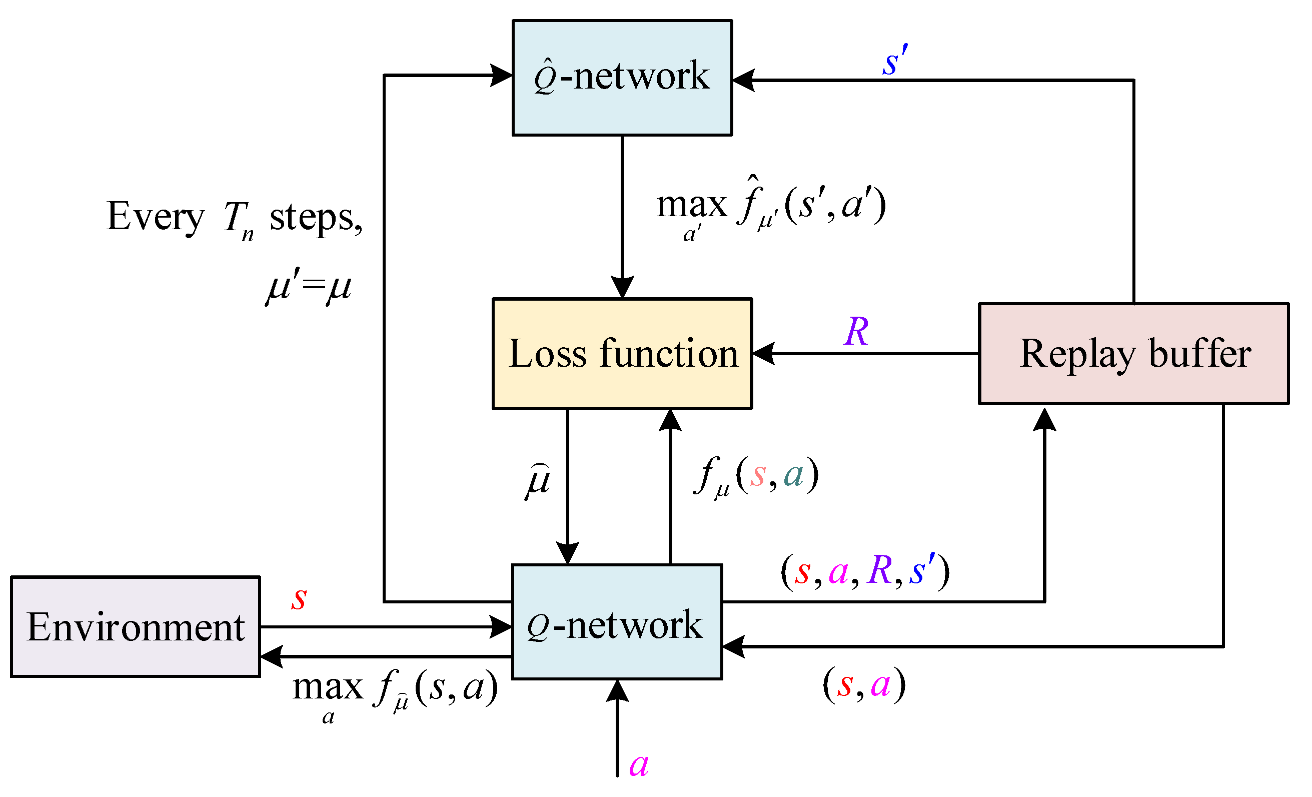
The dimensionality of the state space limits the Q-learning, and training is difficult when the state space is large. Therefore, a DQN is generated based on Q-learning, which uses a neural network to represent the Q table. That is, f μ s , a Q s , a , where f is the output of the neural network with weight μ . It should be pointed out that the input of the neural network is the system state, and the output is the f μ s , a corresponding to the actions. The structure diagram of the DQN is shown in Figure 3.
As shown in Figure 3, there are two neural networks in total, namely, the Q-network and the target Q ^ -network. The data for neural network training comes from the replay buffer. The weight of the Q-network is μ , which is updated by the loss function
J = E s , a , R , s D R + γ max a f μ s , a f μ s , a 2 ,
where s and a correspond to the state s and action a of the next moment, respectively. μ is the weight of the target network, and it is updated periodically. In other words, the weight of the target network does not need to be updated through training, while the weight of the Q-network can be updated according to the gradient descent method, shown as follows:
μ = μ + α [ R + γ max a f μ ( s , a ) f μ ( s , a ) ] f μ ( s , a ) ,
where α is the learning rate. In addition, Equation (35) can be understood as the cost function in DQN, which is to minimize the error between the actual Q ( s , a ) : R + γ max a f μ ( s , a ) value and the estimated Q ( s , a ) : f μ ( s , a ) . Then, the optimal parameters can be selected by the estimated Q that is close to the true Q value.

4.2. Design of Agent Based on Parafoil System

According to the above description, we must first define the system’s state and provide an action space. For the parafoil system, since we expect the parafoil system to fly along the desired path, Δ d and Δ d ˙ define the state of the environment. In other words, at time t, the system will generate two state values:
s 01 t = Δ d , s 02 t = Δ d ˙ .
As for the action space, the parameters that need to be adjusted are ω o and ω c , so the action space is obtained by permutation and combination based on these two parameters. The action space of ω o and ω c is expressed as
ω o ω o min , ω o max ω c ω c min , ω c min ,
where the sampling interval is h for the two parameters. This means that ω o and ω c are N ω o = ω o max ω o min h + 1 and N ω c = ω c max ω c min h + 1 , respectively. Therefore, the dimension of the action space is N ω o N ω c .
The reward function is a direct factor that affects the agent’s training. In order to enable the parafoil system to track the desired path better, we hope that when Δ d is relatively small, the reward function can be significant. Therefore, the reward function in this paper is designed as
R = 10 s i g n s 1 2 s 2 .
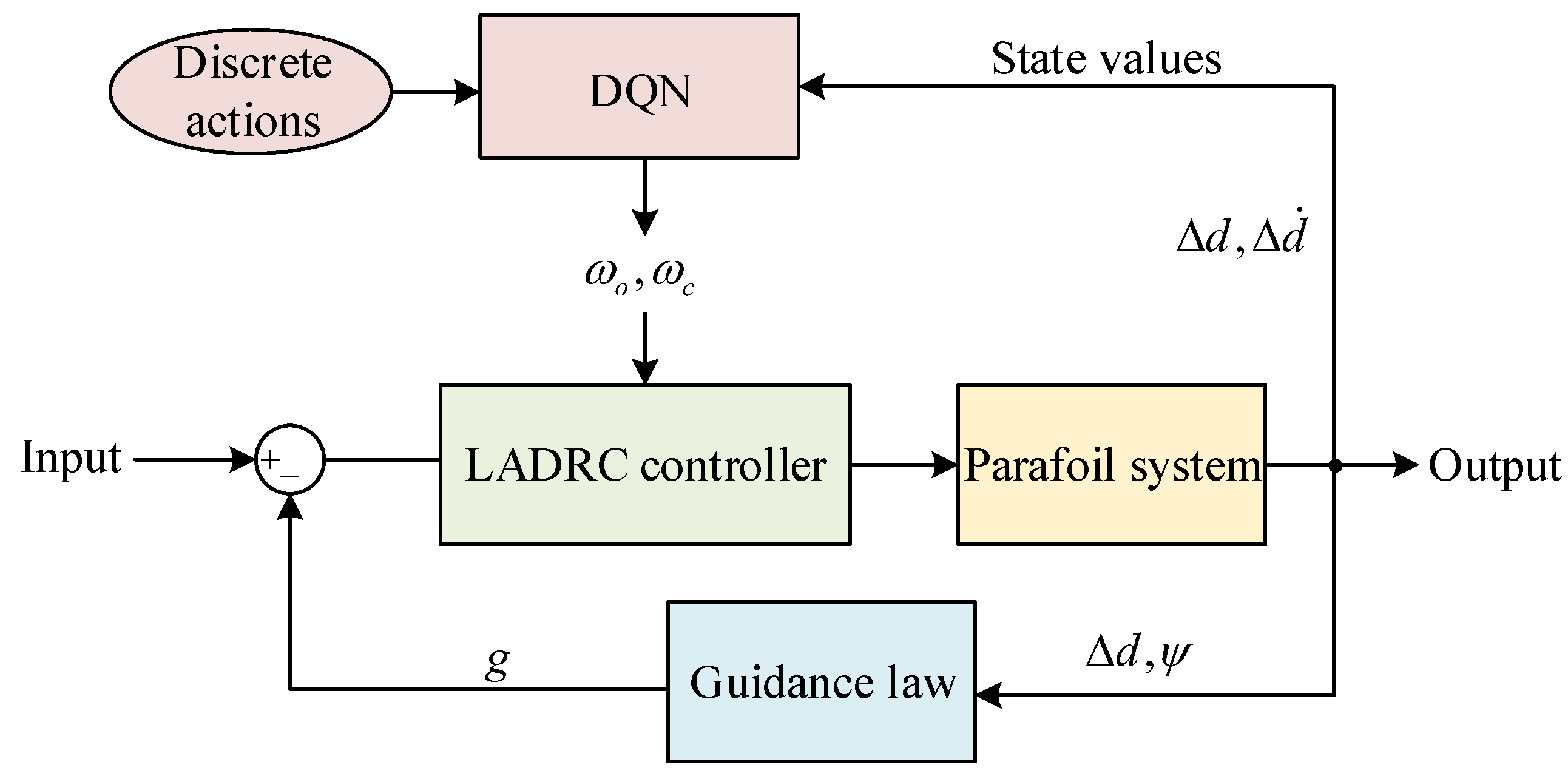
The reward function means that when Δ d is less than 2, the agent can obtain a reward of 10. Otherwise, it can obtain a reward of −10. The smaller Δ d ˙ is, the greater the reward is. The training process of the DQN is described in Algorithm 1. The schematic diagram of the parameter optimization based on the DQN is shown in Figure 4. It should be pointed out that the process of optimizing the LADRC controller parameters by the DQN algorithm includes two parts: offline training, shown in Algorithm 1, and online parameter acquisition. During offline training, a Q-network is obtained, and the training time is related to the simulation sample step and the number of iterations. The smaller the simulation sample step is or the larger the number of iterations is, the longer the training time will be. Moreover, by inputting the system state at the current moment into the trained Q-network, the optimal action values can be obtained to realize adaptive controller parameters, which is the online parameter selection process.
Algorithm 1: DQN algorithm.
  1:
Initialize the replay buffer; Initialize the Q-network with random weights μ ; Initialize the target Q ^ -network with weights μ = μ .
  2:
for episode = 1:M do
  3:
    Initialize the states s 1 = s 01 , s 02 ;
  4:
    for t = 1:T do
  5:
    Select a random action a t = ω o , ω c with the probability ε ; otherwise, select a t = arg max a f μ s t , a ;
  6:
    Execute action a t in the LADRC and observe the reward R t and s t + 1 ;
  7:
    Set s t + 1 = s t ;
  8:
    Store ( s t , a t , R t , s t + 1 ) in the replay buffer D ;
  9:
    Randomly extract m sets of data ( s j , a j , R j , s j + 1 ) from the replay buffer D ;
10:
    Set y j = R j , if episode terminates at step j + 1 R j + γ max a f μ s j + 1 , a j + 1 , otherwise
11:
    Perform a gradient descent step according to Equation (36);
12:
    Every T n steps, reset μ = μ .
13:
    end for
14:
end for

5. Simulation and Analysis

5.1. Environment Setting

In this section, the effectiveness of the proposed DQN-LADRC method is verified by simulations. The parafoil system’s parameters are shown in Table 1. In addition, the parameters involved in the DQN training process are shown in Table 2, where the Q-network is a fully connected neural network with two hidden layers. The network’s inputs are the state values shown in Equation (37), and the outputs are the parameters to be optimized. Both hidden layers have 500 neurons. In addition, the learning rate value was fixed during training, and its value was small enough to ensure convergence of the networks.
Furthermore, the range limits of the parameter tuning in this paper were artificially selected to ensure that the simulation could proceed smoothly within the selected range. The change of the parameter range size, on the one hand, could cause the system to directly stop the training when the “bad” parameters were explored; on the other hand, if the parameter range was too large, it would greatly increase the training time unnecessarily.
It should also be noted that, since the state observer will have extreme values in the transient response, to avoid adverse effects on equipment caused by extreme values, the control quantity generated by the motor connecting the control rope of the dynamic parafoil is limited: 1 u 1 [32].

5.2. Performance Study of DQN-LADRC under Wind Disturbances

5.2.1. Circular Path Following

In order to verify the effectiveness of the proposed method, the DNQ-LADRC-based lateral path-following control of the parafoil system was conducted under wind disturbances. The desired path was set as a circle with a center of (0 m, 0 m) and a radius of 200 m. In the initial state, the three coordinates coincided, and the initial velocity and angular velocity of the parafoil were V s = 14.9 , 0 , 2.1 T m/s and W s = 0 , 0 , 0 T rad/s, respectively. Furthermore, the parafoil’s initial plane position and initial heading angle were (0 m, 150 m) and 0 , respectively. In the simulation environment, the average wind speed of 2 m/s along the y-axis square of the ground coordinate system was added at 50 s, and the duration was 20 s. g 0 , g 1 , and b 0 were selected as 0.08, 0.2, and 0.2, respectively. This paper compares the control effect of the proposed method with the traditional LADRC controller under a wind disturbance of the same size and direction, in which the parameters of the LADRC were selected from two sets of boundary values of the action space, as follows:
ω o 1.5 , 2.7 , ω c 0.4 , 1 , For DQN - LADRC , h = 0.01 ω o = 2.7 , ω c = 1 , For LADRC 1 ω o = 1.5 , ω c = 0.4 , For LADRC 2 .
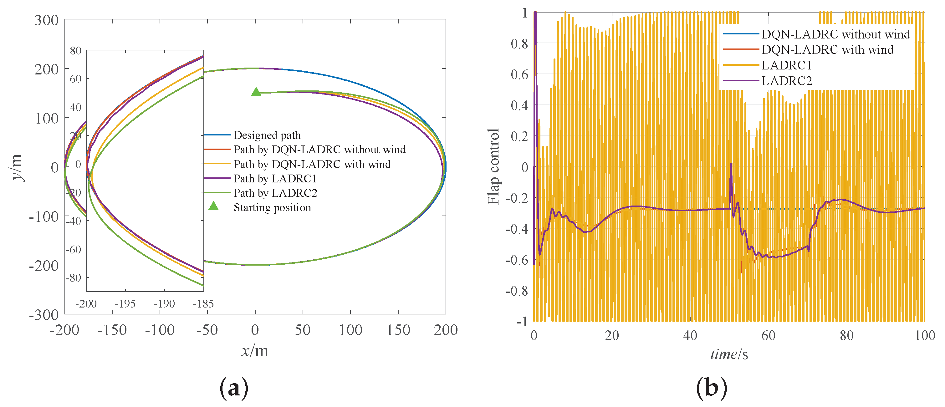
The abovementioned trained agent was used to obtain the parameters of ω o and ω c , and the simulation results are shown in Figure 5, Figure 6, Figure 7 and Figure 8.
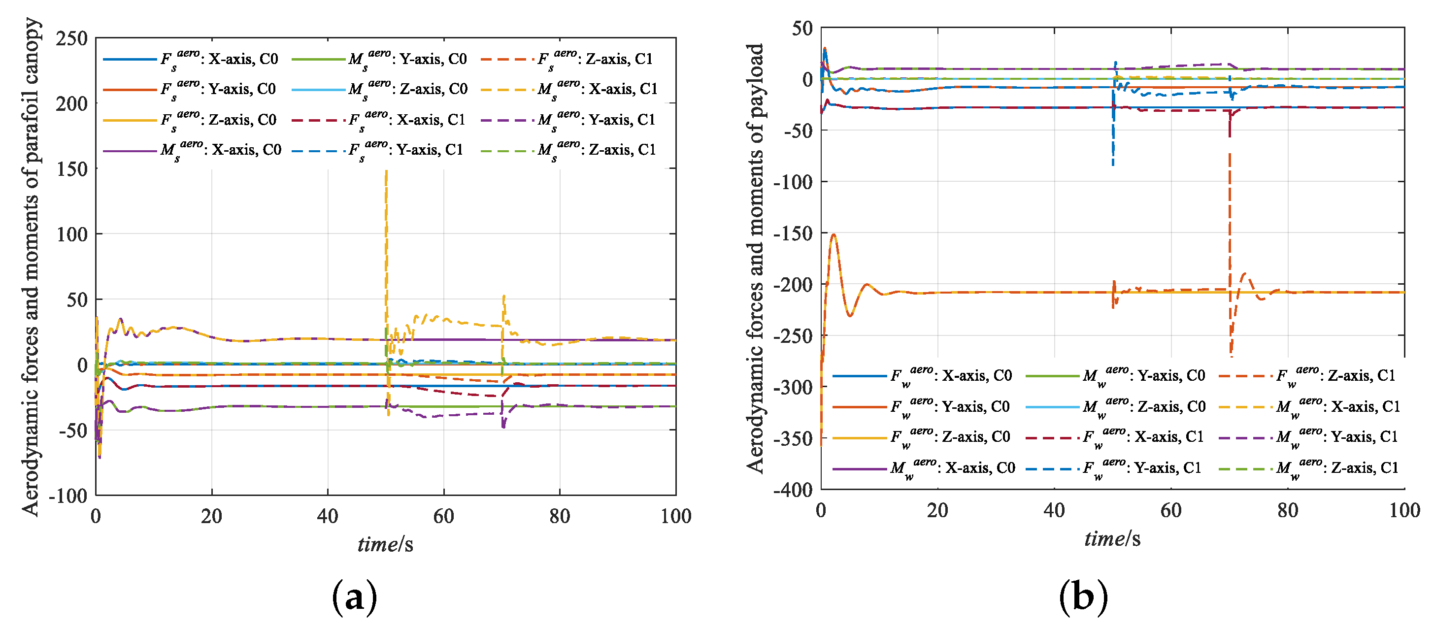
Figure 5 shows the intuitive effect of the parafoil tracking of the desired path with and without wind disturbances, respectively. We can see that both the DQN-LADRC and the traditional LADRC could overcome disturbances and achieve circular path tracking. Specifically, the proposed method achieved better results than the LADRC with the fixed parameters in terms of the control variables, as shown in Figure 5b, and the tracking errors, as shown in Figure 6. It can be found that when the smaller controller parameters were taken, the overshoot of the tracking error obtained by the LADRC was more significant. For more extensive controller parameters, although the overshoot became smaller, the system shock could not be ignored, and such drastic changes in the flap deflection could not be realized in practice. The Euler angles in Figure a show the flight attitude of the parafoil during path tracking. From Figure b, we can observe that the agent had significantly different action values under the influence of wind disturbances. This is also the core idea of the proposed method: to adjust the controller parameters in real time according to the system state. Figure 8 shows the aerodynamic forces and moments of parafoil canopy and payload in three coordinate axes.

5.2.2. Straight Path Following

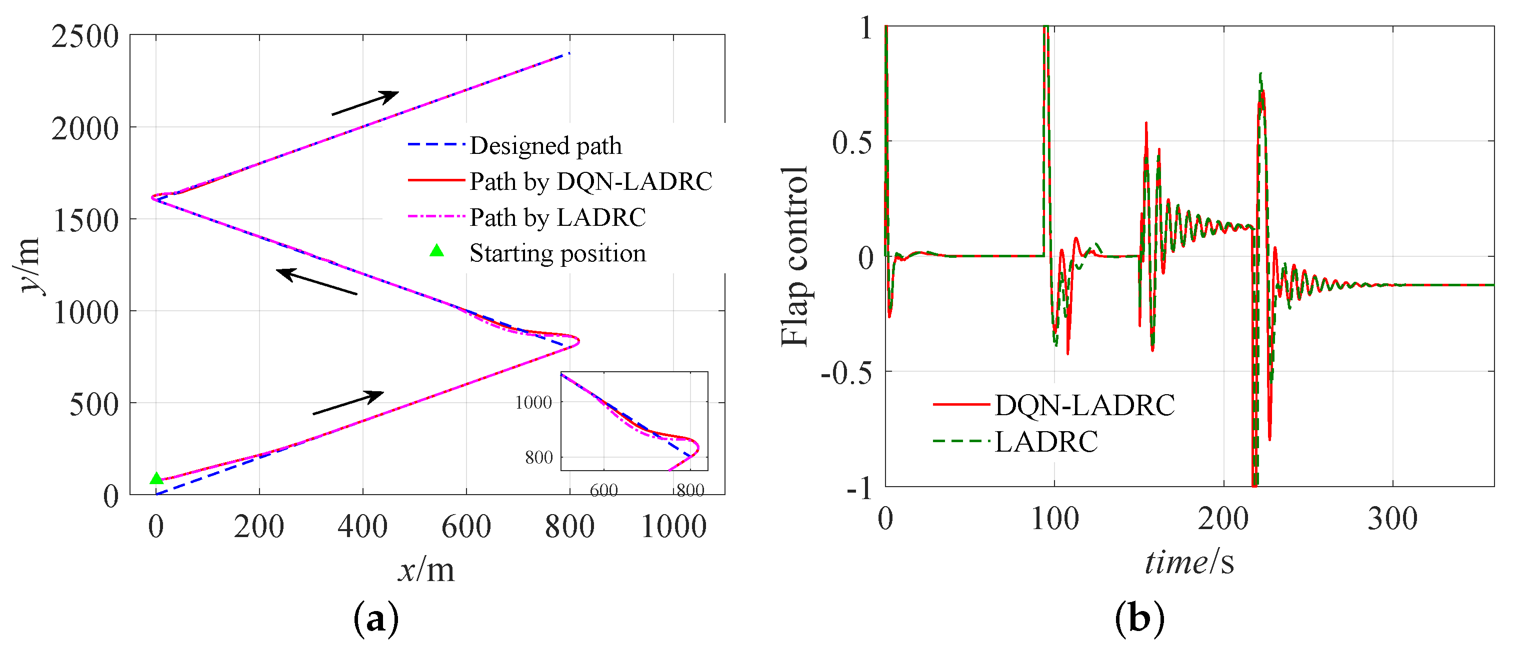
To prove that the above results were not accidental, the straight-path-following control for the parafoil system was also studied. The desired path consisted of three line segments, and the initial position of the parafoil was (0, 80 m). With the initial heading angle of 0 and b 0 of 0.2, the simulation results by the DQN-LADRC are shown in Figure 9, Figure 10, Figure 11 and Figure 12. In order to reflect the anti-interference performance of the proposed method, a south wind of 5 m/s was added at 150 s and continued until the end of the simulation.
Figure 9 shows the tracking effect of the straight path. It can be seen that the system continuously adjusted the flight direction by controlling the rope after being affected by the wind. It can be observed from Figure 10 that the parafoil could fly according to the planned heading angle, and its attitude angles could finally be stabilized. That is, the parafoil could smoothly follow the designed path. The path tracking error is shown in Figure 11a, where the path tracking deviation was 0 at steady state. In addition, the parafoil had large tracking deviations during sharp turns. The adaptive controller parameters are given in Figure 11b, where ω o [ 0.5 , 1.5 ] and ω c [ 0.2 , 0.5 ] , with sampling intervals of 0.01. To demonstrate the proposed method’s effectiveness, the LADRC controller’s control effect with fixed parameters of ω o = 1.5 and ω c = 0.5 was added to the results. The aerodynamic forces and moments on the canopy and payload are shown in Figure 12 in three coordinate axes. It can be seen that in the z-axis direction there are aerodynamic effects. This is because in the eight-DOF model in this paper, we default that the parafoil is free-falling in the longitudinal direction. Even so, the proposed method can enable the parafoil to track a given path on the plane.
By comparing the tracking effect of the circular path and the straight path, it can be seen that the tracking effect of the straight path was better. This was because the guidance law is based on the idea of tracking a straight line. In circular path tracking, a circle is approximated as an infinite number of straight line segments.

6. Conclusions

This paper studied the lateral path-following control of the parafoil system. First, an eight-DOF dynamic model of the parafoil system was constructed, considering the relative motion between the parafoil canopy and the payload. Then, using the error conversion between the parafoil system’s position information and the desired path, a guidance law was proposed, which essentially converts the path following into the control of the parafoil system’s heading angle. Furthermore, a second-order LADRC was designed based on the guidance law, and the DQN was applied to optimize the controller parameters adaptively. Finally, the proposed DNQ-LADRC was applied to control the parafoil system to follow a circular path under environments with and without disturbances and a straight path under wind disturbances. The simulation results demonstrated that the influence of wind disturbances on the parafoil could not be ignored. The proposed method could overcome the effect of wind disturbances and realize the tracking control of straight or circular paths. Compared with the traditional LADRC controller, the proposed method has certain advantages in terms of the settling time and overshoot.
In future work, we will simultaneously consider implementing lateral and longitudinal path tracking control of the parafoil system and applying the proposed method to actual experiments for verification. In addition, the DQN can realize the optimization of controller parameters, but it also requires human experience to divide the action space. The agent training of the DQN will be difficult when the action space is too large. Therefore, one of our goals is to explore a fully intelligent reinforcement learning algorithm. In this study, only the disturbances caused by uniform wind were considered, but in the actual flight process, the parafoil system will be affected by various complex wind fields. Thus, path-following control of the parafoil based on wind field identification is what we hope to achieve.

Author Contributions

Conceptualization, Y.Z. and J.T.; Methodology, Y.Z. and H.S.; Software, Y.Z.; Validation, Q.S. and Z.C.; Formal analysis, Y.Z.; Writing—original draft preparation, Y.Z.; Writing—review and editing, J.T.; Supervision, J.T., Q.S., H.S., M.S. and F.D.; Funding acquisition, J.T. All authors have read and agreed to the published version of the manuscript.

Funding

This work was supported by the National Natural Science Foundation of China (Grant Nos. 61973172, 61973175, 62003175, and 62003177), the National Key Research and Development Project (Grant No. 2019YFC1510900), and the Key Technologies Research and Development Program of Tianjin (Grant No. 19JCZDJC32800). This project was also funded by China Postdoctoral Science Foundation (Grant No. 2020M670633) and Tianjin Postgraduate Research and Innovation Project 2021YJSB084.

Institutional Review Board Statement

Not applicable.

Informed Consent Statement

Not applicable.

Data Availability Statement

Data sharing not applicable.

Conflicts of Interest

The authors declare that they do not have any conflicts of interest.

References

  1. Zhu, H.; Sun, Q.; Liu, X.; Liu, J. Fluid–structure interaction-based aerodynamic modeling for flight dynamics simulation of parafoil system. Nonlinear Dyn. 2021, 104, 3445–3466. [Google Scholar] [CrossRef]
  2. Guo, Y.; Yan, J.; Wu, C.; Xiao, B. Modeling and practical fixed-time attitude tracking control of a paraglider recovery system. ISA Trans. 2022, 128, 391–401. [Google Scholar] [CrossRef] [PubMed]
  3. Slegers, N.; Costello, M. Model predictive control of a parafoil and payload system. J. Guid. Control Dyn. 2005, 28, 816–821. [Google Scholar] [CrossRef]
  4. Zhang, Z.; Zhao, Z.; Fu, Y. Dynamics analysis and simulation of six DOF parafoil system. Clust. Comput. 2018, 22, 12669–12680. [Google Scholar] [CrossRef]
  5. Zhu, E.; Sun, Q.; Tan, P.; Chen, Z. Modeling of powered parafoil based on Kirchhoff motion equation. Nonlinear Dyn. 2014, 79, 617–629. [Google Scholar] [CrossRef]
  6. Tan, P.; Sun, M.; Sun, Q.; Chen, Z. Dynamic modeling and experimental verification of powered parafoil with two suspending points. IEEE Access 2020, 8, 12955–12966. [Google Scholar] [CrossRef]
  7. Prakash, O. NDI based generic heading tracking control law for parafoil/payload system. In Proceedings of the AIAA Aviation 2020 Forum, Virtual Event, 15–19 June 2020. [Google Scholar] [CrossRef]
  8. Tao, J.; Dehmer, M.; Xie, G.; Zhou, Q. A generalized predictive control-based path following method for parafoil systems in wind environment. IEEE Access 2019, 7, 42586–42595. [Google Scholar] [CrossRef]
  9. Zhao, L.; He, W.; Lv, F. Model-free adaptive control for parafoil systems based on the iterative feedback tuning method. IEEE Access 2021, 9, 35900–35914. [Google Scholar] [CrossRef]
  10. Guo, Y.; Yan, J.; Wu, C.; Wu, X.; Chen, M.; Xing, X. Autonomous homing design and following for parafoil/rocket system with high-altitude. J. Intell. Robot. Syst. 2021, 101, 73. [Google Scholar] [CrossRef]
  11. Li, Y.; Zhao, M.; Yao, M.; Chen, Q.; Guo, R.; Sun, T.; Jiang, T.; Zhao, Z. 6-DOF modeling and 3D trajectory tracking control of a powered parafoil system. IEEE Access 2020, 8, 151087–151105. [Google Scholar] [CrossRef]
  12. Tao, J.; Sun, Q.; Sun, H.; Chen, Z.; Dehmer, M.; Sun, M. Dynamic modeling and trajectory tracking control of parafoil system in wind environment. IEEE ASME Trans. Mechatron. 2017, 22, 2736–2745. [Google Scholar] [CrossRef]
  13. Tao, J.; Liang, W.; Sun, Q.; Tan, P.; Luo, S.; Chen, Z.; He, Y. Modeling and control of a powered parafoil in wind and rain environments. IEEE Trans. Aerosp. Electron. Syst. 2017, 53, 1642–1659. [Google Scholar] [CrossRef]
  14. Han, J. From PID to active disturbance rejection control. IEEE Trans. Ind. Electron. 2019, 56, 900–906. [Google Scholar] [CrossRef]
  15. Han, J. Auto-disturbance-rejection controller and its applications. Contr. Decis. 1998, 13, 19–23. [Google Scholar]
  16. Gao, Z. On the foundation of active disturbance rejection control. Control. Theory Appl. 2013, 30, 1498–1510. [Google Scholar]
  17. Chen, Z.; Wang, Y.; Sun, M.; Sun, Q. Convergence and stability analysis of active disturbance rejection control for first-order nonlinear dynamic systems. Trans. Inst. Meas. Control 2019, 41, 2064–2076. [Google Scholar] [CrossRef]
  18. Wang, Y.; Chen, Z.; Sun, M.; Sun, Q. On the stability and convergence rate analysis for the nonlinear uncertain systems based upon active disturbance rejection control. Int. J. Robust Nonlinear Control 2020, 30, 5728–5750. [Google Scholar] [CrossRef]
  19. Zheng, Y.; Chen, Z.; Huang, Z.; Sun, M. Active disturbance rejection controller for multi-area interconnected power system based on reinforcement learning. Neurocomputing 2021, 425, 149–159. [Google Scholar] [CrossRef]
  20. Zheng, Y.; Tao, J.; Sun, H.; Sun, Q. An intelligent course keeping active disturbance rejection controller based on Double Deep Q-network for towing system of unpowered cylindrical drilling platform. Int. J. Robust Nonlinear Control 2021, 31, 8463–8480. [Google Scholar] [CrossRef]
  21. Tao, J.; Du, L.; Dehmer, M.; Wen, Y. Path following control for towing system of cylindrical drilling platform in presence of disturbances and uncertainties. ISA Trans. 2019, 95, 185–193. [Google Scholar] [CrossRef]
  22. Zeng, D.; Yu, Z.; Xiong, L.; Fu, Z.; Li, Z. HFO-LADRC lateral motion controller for autonomous road sweeper. Sensors 2020, 20, 2274. [Google Scholar] [CrossRef] [PubMed]
  23. Liu, C.; Luo, G.; Duan, X. Adaptive LADRC-based disturbance rejection method for electromechanical servo system. IEEE Trans. Ind. Appl. 2020, 56, 876–889. [Google Scholar] [CrossRef]
  24. Li, R.; Li, T.; Bu, R.; Zheng, Q.; Chen, C.L. Active disturbance rejection with sliding mode control-based course and path following for underactuated ships. Math. Probl. Eng. 2013, 2013, 743716-1–743716-9. [Google Scholar] [CrossRef] [Green Version]
  25. Zhao, P.; Nagamune, R. Switching linear parameter-varying control with improved local performance and optimized switching surfaces. Int. J. Robust Nonlinear Control 2018, 28, 3403–3421. [Google Scholar] [CrossRef]
  26. Li, Y.; Jia, M.; Han, X. Towards a comprehensive optimization of engine efficiency and emissions by coupling artificial neural network (ANN) with genetic algorithm (GA). Energy 2021, 225, 120331. [Google Scholar] [CrossRef]
  27. Ho, S.; Shu, L. Optimizing fuzzy neural networks for tuning PID controllers using an orthogonal simulated annealing algorithm OSA. IEEE Trans. Fuzzy Syst. 2006, 14, 421–434. [Google Scholar] [CrossRef]
  28. Sun, C.; Liu, M.; Liu, C.A.; Feng, X.; Wu, H. An industrial quadrotor UAV control method based on fuzzy adaptive linear active disturbance rejection control. Electronics 2021, 10, 376. [Google Scholar] [CrossRef]
  29. Mnih, V.; Kavukcuoglu, K.; Silver, D. Human-level control through deep reinforcement learning. Nature 2015, 518, 529–533. [Google Scholar] [CrossRef]
  30. Zhao, Y.; Qi, X.; Ma, Y.; Li, Z.; Malekian, R.; Sotelo, M.A. Path following optimization for an underactuated USV using smoothly-convergent deep reinforcement learning. IEEE Trans. Intell. Transp. Syst. 2020, 22, 1–13. [Google Scholar] [CrossRef]
  31. Xue, W.; Huang, Y. Performance analysis of active disturbance rejection tracking control for a 513 class of uncertain LTI systems. ISA Trans. 2015, 58, 133–154. [Google Scholar] [CrossRef]
  32. Sun, Q.; Yu, L.; Zheng, Y.; Tao, J.; Sun, H.; Sun, M.; Dehmer, M.; Chen, Z. Trajectory tracking control of powered parafoil system based on sliding mode control in a complex environment. Aerosp. Sci. Technol. 2022, 122, 107406. [Google Scholar] [CrossRef]
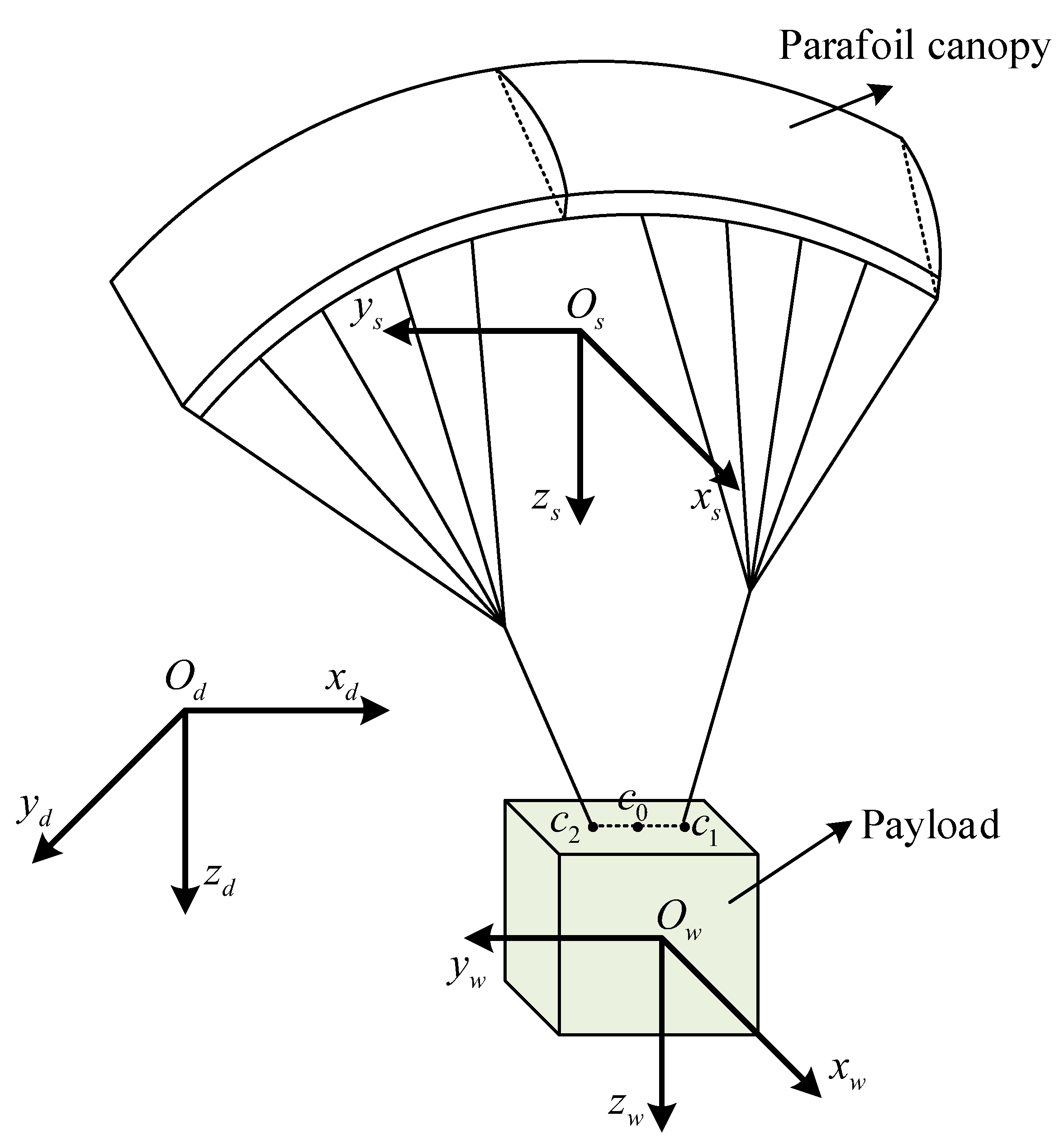
Figure 1. Schematic diagram of parafoil system coordinates.
Sustainability 15 00435 g001
Figure 2. Schematic diagram of path following.
Sustainability 15 00435 g002
Figure 3. Structure diagram of deep Q-network (DQN).
Sustainability 15 00435 g003
Figure 4. DQN-based linear active disturbance rejection controller (LADRC) control structure diagram.
Sustainability 15 00435 g004
Figure 5. Circular-path-following control results. (a) Path-following trajectories. (b) Control variables.
Sustainability 15 00435 g005
Figure 6. Circular-path-following control results of attitude angles. (a) Heading angle. (b) Position deviation.
Sustainability 15 00435 g006
Figure 7. Variation process of Euler angles and controller parameters for circular-path-following control. (a) Euler angles. (b) Adaptive parameters.
Sustainability 15 00435 g007
Figure 8. Changing process of aerodynamic forces and moments of parafoil canopy and payload for circular path following. (a) F s a e r o and M s a e r o in two conditions. C0: the system is not disturbed by wind; C1: the system is disturbed by wind. (b) F w a e r o and M w a e r o in two conditions. C0: the system is not disturbed by wind; C1: the system is disturbed by wind.
Sustainability 15 00435 g008
Figure 9. Straight-path-following control results under wind disturbances. (a) Path-following trajectories. (b) Control variables.
Sustainability 15 00435 g009
Figure 10. Straight-path-following control results of attitude angles under wind disturbances. (a) Heading angles. (b) Euler angles.
Sustainability 15 00435 g010
Figure 11. Tracking error and adaptive controller parameters. (a) Position derivation. (b) Controller parameters.
Sustainability 15 00435 g011
Figure 12. Changing process of aerodynamic forces and moments of parafoil canopy and payload for straight path following. (a) F s a e r o and M s a e r o . (b) F w a e r o and M w a e r o .
Sustainability 15 00435 g012
Table 1. Physical parameters of the parafoil system.
Parameter DescriptionValue
Wing span4.5 m
Mean aerodynamic chord1.3 m
Mass of parafoil1.7 kg
Mass of payload20 kg
Wing area6.5 m 2
Rope length3 m
Table 2. Parameter settings of DQN.
Parameter DescriptionValue
Simulation sample step0.02 s
Number of iterations300
Learning rate of Q-network 10 4
Discount factor0.99
Disclaimer/Publisher’s Note: The statements, opinions and data contained in all publications are solely those of the individual author(s) and contributor(s) and not of MDPI and/or the editor(s). MDPI and/or the editor(s) disclaim responsibility for any injury to people or property resulting from any ideas, methods, instructions or products referred to in the content.