A Novel Linguistic Interval-Valued Pythagorean Fuzzy Multi-Attribute Group Decision-Making for Sustainable Building Materials Selection

Abstract

The linguistic interval-valued Pythagorean fuzzy (LIVPF) sets, which absorb the advantages of linguistic terms set and interval-valued Pythagorean fuzzy sets, can efficiently describe decision makers’ evaluation information in multi-attribute group decision-making (MAGDM) problems. When investigating aggregation operators of linguistic interval-valued Pythagorean fuzzy (LIVPF) information, we have to consider two important issues, viz. the operational rules of LIVPF numbers and aggregation functions. The classical Archimedean t-norm and t-conorm (ATT) are a famous t-norm and t-conorm, which can produce some special cases. Recently, ATT has been widely applied in different fuzzy decision-making information. Hence, in this paper, for the first issue, we propose some novel operational rules of LIVPF numbers based on ATT. The new operational laws are flexible and can generate some useful operations. For the second issue, we choose a powerful function, i.e., the extended power average (EPA) operator as the aggregation function. The prominent advantages of EPA are that it not only considers the relationship among input arguments, but also dynamically changes the weights of input arguments by employing a parameter. Hence, our proposed novel aggregation operators for LIVPFNs are flexible and is suitable to handle MAGDM problems in actual life. Afterward, we further present a novel MAGDM method under LIVPF conditions. The main finding of our study is a new MAGDM method, which is more powerful and flexible than existing ones. Finally, we apply the method in a sustainable building materials selection to show its effectiveness. Additionally, comparison analysis is provided to demonstrate the advantages and superiorities of the proposed method.

1. Introduction

With the continuous development of urbanization, a large number of people have poured into cities, which has promoted the rapid development of the construction and building industry. As the concept of environmental protection has been realized by people, environmental protection issues in the construction industry have also received increasing attention. Many areas of the construction industry need to pay attention to environmental protection and sustainability, and among which the selection of sustainable building materials is one of the most important. Sustainable building materials refer to materials that are friendly to the environment and do not harm human health and comfort. Therefore, in the construction industry, how to choose suitable environmental protection materials is a topic worthy of in-depth study. The selection of sustainable materials is not easy as many factors need to be taken into consideration. Recently, more and more scholars have studied sustainable building materials selection (SBMS) problem from the perspective of multi-attribute group decision-making (MAGDM). For instance, Akadiri et al. [1] proposed criteria for evaluating sustainability of building materials for construction projects and put forward a fuzzy analytic hierarchy process method for SBMS. Similarly, Mahmoudkelaye et al. [2] studied SBMS problems from the perspective of the analytic network process. Roy et al. [3] introduced a CODAS based MAGDM method under the interval-valued intuitionistic fuzzy environment and applied in the SBMS. Meng and Dong [4] developed the linguistic intuitionistic fuzzy PROMETHEE method to determine the most suitable materials for indoor flooring. Chen et al. [5] proposed a hybrid decision-making method by integrating QFD and ELECTRE-III and studied its application in SBMS. Similarly, Khoshnava et al. [6] studied SBMS based on a novel hybrid decision-making method, which integrates DEMATEL and a fuzzy analytic network process. Ahmed et al. [7] presented an OSM-AHP-TOPSIS method for solving SBMS problems. Chen et al. [8] investigated SBMS methods under a large group decision-making context. For a more recent development of group decision-making based SBMS methods, readers are suggested to refer to [9], where authors conducted a systematic literature review on this topic.

The above-mentioned MAGDM methods have been proven to be effective to deal with SBMS problems. However, as SBMS problems have become more and more complex, these methods are still insufficient to deal with realistic SBMS problems. For instance, in [1], the authors developed a fuzzy hierarchy process method for SBMS. However, sometimes, fuzzy sets are inadequate to describe decision makers’ (DMs’) evaluation information as they only have membership degrees. Roy et al. [3] introduced an interval-valued intuitionistic fuzzy MAGDM method-based approach for handling SBMS problems. However, this method still has limitations and, in realistic SBMS problems, DMs would like to use linguistic membership and non-membership degrees to express their evaluation opinions. In [4], Meng and Dong developed a linguistic intuitionistic fuzzy MAGDM method for dealing with SBMS problems. Nevertheless, the constraint of linguistic intuitionistic fuzzy sets is that the sum of linguistic scripts should be less than or equal to the length of the pre-defined linguistic terms set, which cannot be always satisfied in modern realistic SBMS problems. Hence, Meng and Dong’s study [4] still has some limitations. To fill this gap, novel MAGDM methods should be developed for modern and complex SBMS problems. As a matter of fact, MAGDM is one of the important branches of decision science, which represents the process of considering decision information to obtain the most desirable choice. Furthermore, how DMs give the evaluation values and how to rank all alternatives are two pivotal processes. Scholars usually focus on these two points, explore a variety of MAGDM methods [10,11,12,13,14], and apply them to quite a few realistic decision-making problems. For the evaluation value of attributes given by DMs, the concept of fuzzy sets is presented and becomes a powerful tool to solve the MAGDM problem. As the complexity and ambiguity of the actual decision-making environment increases, the DMs use various forms of evaluation values, such as “good”, “very good”, “fair”, “poor”, and “very poor”. Therefore, Zadeh [15,16] came up with the concept of linguistic variables (LVs), replacing numbers to express ambiguous information of DMs. After that, LVs were introduced into various fuzzy sets to better deal with uncertain information in MAGDM, such as intuitionistic fuzzy sets (IFSs) [17] and Pythagorean fuzzy sets (PFSs) [18]. In detail, Zhang [19] proposed linguistic intuitionistic fuzzy sets (LIFSs), which combines the strengths of IFSs and LVs. Furthermore, Garg [20] presented the concept of a linguistic Pythagorean fuzzy set (LPFS) characterized by a linguistic membership degree (LMD) and a linguistic non-membership degree (LNMD). Based on LPFS, many aggregation operators (AOs) and typical decision-making methods were extended to solve the MAGDM problem [21,22,23,24,25], and were applied in real decision-making environments.

The cognitive structure of DMs is limited, and the decision environment is uncertain. Therefore, using interval values instead of single linguistic variable to represent the membership degree (MD) and non-membership degree (NMD) can describe the preference information of DMs more conveniently and freely. Some extension of fuzzy sets combined with interval values to describe fuzzy information [26,27,28]. For example, Liu et al. [26] integrated the best–worst method and alternative queuing method within the interval-valued intuitionistic uncertain linguistic setting and applied the proposed method in sustainable supply chain management. Mu et al. [27] proposed a novel MAGDM method with a new comparison rule for interval-valued Pythagorean fuzzy numbers, which can capture the interaction between attributes. By combining LVs and interval values, a wider range of information can be described. Garg [28] presented an extension of PFSs called linguistic interval-valued Pythagorean fuzzy sets (LIVPFSs), which characterized the membership and non-membership degrees as the interval-valued linguistic terms to represent ambiguous assessment information. Meanwhile, a new MAGDM method was proposed based on several weighted averages and geometric aggregating operators, including linguistic interval-valued Pythagorean fuzzy weighted averaging (LIVPFWA) operator and linguistic interval-valued Pythagorean fuzzy weighted geometric (LIVPFWG) operator.

The MAGDM methods based on LIVPFSs provide a wider space of fuzzy information for DMs, but there are still the following two deficiencies: the operational laws and the aggregation functions. Firstly, the operational laws based on LIVPFSs used to assemble assessment values of attributes were singly proposed by Garg [28]. However, this complicated aggregation process requires flexible operational laws in practical decision-making problems. Consequently, we introduce the Archimedean T-norm and T-conorm (ATT) into LIVPFSs and propose novel operational laws. It is widely known that ATT is the generalization of a lot of T-norm (TN) and T-conorm (TC), which have special and important members. A lot of operational laws based on the special cases of ATT were proposed, such as Einstein operational laws, Hamacher operational laws, Frank operational laws, Dombi operational laws, and so on. In 2011, Beliakov et al. [29] developed some operations with IFSs based on ATT, and proposed an aggregation principle for fuzzy information. Gradually, Wang and Garg [30] defined certain interactive operational rules on PFSs with the aid of ATT. In addition, Qin et al. [31] proposed a series of aggregation operators based on ATT under LIVIFSs to solve the situation in which the operational laws of aggregation information are inflexible. Motivated by this, we combine the characteristics of ATT with LIVPFSs to describe a larger information space, and provide DMs with a variety of flexible operational laws to choose.

Another point, in terms of aggregation functions, the proposed MAGDM methods based on LIVPFSs [28] cannot effectively deal with the extreme evaluation values given by DMs. Therefore, it is necessary to develop an effective information aggregation method to eliminate the influence of extreme evaluation values of DMs and obtain more reasonable rankings of alternatives. Yager [32] proposed the power average (PA) operator to deal with unreasonable evaluation values by assigning small weights to extreme evaluation values. Likewise, the power geometric (PG) operator was proposed by Xu and Yager [33], which also can reduce the effects of unreasonable values. PA and PG operators are also widely used in multi-attribute decision-making problems [34,35]. However, extreme or unreasonable assessment values may be important and critical decision-making information under different circumstances. Based on this, Xiong et al. [36] extended the PA operator to expand its application in decision-making problems by setting different input parameters, and proposed an extended power average (EPA) operator and extended power geometric (EPG) operator. The weights of input parameters in EPA and EPG operators can be dynamically adjusted, which enables DMs to focus more on appropriately critical inputs. Li et al. [37] introduced an EPA operator to deal with q-rung dual hesitant fuzzy information, and the validity of this AO was verified. Thus, this is a useful tool to solve the MAGDM problem effectively. In general, it is necessary to combine the EPA operator with LIVPFSs to deal with the MAGDM problem.

The purpose of this paper is to propose a new MAGDM method that can make up for the above two shortcomings, which provides flexible operations and handles extreme evaluation values given by DMs effectively. Thence, the contributions of this paper can be summarized into three points: (1) Combining the advantages of ATT, new operations for LIVPFSs are proposed; (2) Combined with the EPA operator and EPG operator, some AOs of LIVPFSs are presented to deal with unreasonable evaluation information; (3) Based on proposed AOs, a novel MAGDM method is developed to deal with complex decision problems. In order to verify the effectiveness of this method, the method is applied to a numerical example in risk assessment of offshore photovoltaic projects. In addition, the advantages of this method are summarized by comparative analysis. The rest of this paper is organized as follows: Section 2 reviews several basic concepts relevant to this paper. In Section 3, the concept of ATT is introduced and new operations for LIVPFNs based on ATT are proposed. Section 4 proposes new AOs for LIVPFSs, and discusses some properties and special cases. Furthermore, Section 5 presents a novel MAGDM method under LIVPFSs. Section 6 presents a numerical example to illustrate and verify the applicability of the proposed method. A comparative analysis of the results of the numerical example with other existing aggregation operators is also provided in Section 6, and Section 7 concludes the paper.

2. Preliminaries

This section provides a retrospective of some basic concepts that will be used in the following sections.

2.1. The Linguistic Interval-Valued Pythagorean Fuzzy Sets

Definition 1 

([28]). Let X be an ordinary set and $\tilde{S}=\left\{s_{\beta }|s_0\le s_{\beta }\le s_l,\beta \in \left[0,l\right]\right\}$ be a continuous linguistic term set; a linguistic interval-valued Pythagorean fuzzy set (LPFS) A defined on X is expressed as

$$A=\{\langle x,\left[s_a\left(x\right),s_b\left(x\right)\right],\left[s_c\left(x\right),s_d\left(x\right)\right]\rangle |x\in X\},$$

(1)

where $\left[s_a\left(x\right),s_b\left(x\right)\right],\left[s_c\left(x\right),s_d\left(x\right)\right]\subseteq \tilde{S}$ are two uncertain linguistic variables, representing the linguistic interval-valued membership and non-membership degrees of the element $x\in X$ to the set A, such that $b^2+d^2\le l^2$. The ordered pair $\left(\left[s_a\left(x\right),s_b\left(x\right)\right],\left[s_c\left(x\right),s_d\left(x\right)\right]\right)$ is called a linguistic interval-valued Pythagorean fuzzy number (LIVPFN), which can be denoted as $\alpha =\left(\left[s_a,s_b\right],\left[s_c,s_d\right]\right)$.

Garg [28] gave a method to rank any two LIVPFNs.

Definition 2 

([28]). Let $\alpha =\left(\left[s_a,s_b\right],\left[s_c,s_d\right]\right)$ be an LIVPFN defined on a continuous linguistic term set $\tilde{S}=\left\{s_{\beta }|s_0\le s_{\beta }\le s_l,\beta \in \left[0,l\right]\right\}$, the score function of $\alpha$ is expressed as

$$S\left(\alpha \right)=s_{\sqrt{\left(2l^2+a^2+b^2-c^2-d^2\right)/4}},$$

(2)

and the accuracy function of $\alpha$ is expressed as

$$H\left(\alpha \right)=s_{\sqrt{\left(a^2+b^2+c^2+d^2\right)/2}},$$

(3)

For any two LIVPFNs${\alpha }_1=\left(\left[s_{a_1},s_{b_1}\right],\left[s_{c_1},s_{d_1}\right]\right)$and${\alpha }_2=\left(\left[s_{a_2},s_{b_2}\right],\left[s_{c_2},s_{d_2}\right]\right), let$two LIVPFNs be defined on a continuous linguistic term set$\tilde{S}=\left\{s_{\beta }|s_0\le s_{\beta }\le s_l,\beta \in \left[0,l\right]\right\}$; then,

(1)

If $S\left({\alpha }_1\right)>S\left({\alpha }_2\right)$, then ${\alpha }_1>{\alpha }_2$;

(2)

if $S\left({\alpha }_1\right)=S\left({\alpha }_2\right)$, then

• If $H\left({\alpha }_1\right)>H\left({\alpha }_2\right)$, then ${\alpha }_1>{\alpha }_2$;
• If $H\left({\alpha }_1\right)=H\left({\alpha }_2\right)$, then ${\alpha }_1={\alpha }_2$.

Basic operational rules of LIVPFNs are presented as follows.

Definition 3 

([28]). Let ${\alpha }_1=\left(\left[s_{a_1},s_{b_1}\right],\left[s_{c_1},s_{d_1}\right]\right)$, ${\alpha }_2=\left(\left[s_{a_2},s_{b_2}\right],\left[s_{c_2},s_{d_2}\right]\right)$ and $\alpha =\left(\left[s_a,s_b\right],\left[s_c,s_d\right]\right)$ be any three LIVPFNs defined on a pre-defined continuous linguistic term set $\tilde{S}=\left\{s_{\beta }|s_0\le s_{\beta }\le s_l,\beta \in \left[0,l\right]\right\}$, then

(1)

${\alpha }_1\oplus {\alpha }_2=\left(\left[s_{l\sqrt{a_1^2/l^2+a_2^2/l^2-a_1^2{a}_2^2/l^4}},s_{l\sqrt{b_1^2/l^2+b_2^2/l^2-b_1^2{b}_2^2/l^4}}\right],\left[s_{l\left(c_1{c}_2/l^2\right)},s_{l\left(d_1{d}_2/l^2\right)}\right]\right);$

(2)

${\alpha }_1\otimes {\alpha }_2=\left(\left[s_{l\left(a_1{a}_2/l^2\right)},s_{l\left(b_1{b}_2/l^2\right)}\right],\left[s_{l\sqrt{c_1^2/l^2+c_2^2/l^2-c_1^2{c}_2^2/l^4}},s_{l\sqrt{d_1^2/l^2+d_2^2/l^2-d_1^2{d}_2^2/l^4}}\right]\right);$

(3)

$\lambda \alpha =\left(\left[s_{l\sqrt{1-{\left(1-a^2/l^2\right)}^{\lambda }}},s_{l\sqrt{1-{\left(1-b^2/l^2\right)}^{\lambda }}}\right],\left[s_{l{\left(c/l\right)}^{\lambda }},s_{l{\left(d/l\right)}^{\lambda }}\right]\right)$;

(4)

${\alpha }^{\lambda }=\left(\left[s_{l{\left(a/l\right)}^{\lambda }},s_{l{\left(b/l\right)}^{\lambda }}\right],\left[s_{l\sqrt{1-{\left(1-c^2/l^2\right)}^{\lambda }}},s_{l\sqrt{1-{\left(1-d^2/l^2\right)}^{\lambda }}}\right]\right)$.

The distance measure between two LIVPFNs is defined as follows.

Definition 4. 

Let${\alpha }_1=\left(\left[s_{a_1},s_{b_1}\right],\left[s_{c_1},s_{d_1}\right]\right)$and${\alpha }_2=\left(\left[s_{a_2},s_{b_2}\right],\left[s_{c_2},s_{d_2}\right]\right)$be any two LIVPFNs defined on a pre-given continuous linguistic term set$\tilde{S}=\left\{s_{\beta }|s_0\le s_{\beta }\le s_l,\beta \in \left[0,l\right]\right\}$, then the distance between${\alpha }_1$and${\alpha }_2$is expressed as

$$d\left({\alpha }_1,{\alpha }_2\right)=\frac{\left|a_1^2-a_2^2\right|+\left|b_1^2-b_2^2\right|+\left|c_1^2-c_2^2\right|+\left|d_1^2-d_2^2\right|}{4l^2}.$$

(4)

2.2. The Extended Power Average and Extended Power Geometric Operators

Definition 5 

([36]). Let $a_i\left(i=1,2,\dots ,n\right)$ be a collection of real numbers, and an extended power average (EPA) operator of dimension n is a mapping EPA: ${ℛ}^n\to ℛ$, defined by a parameter $\sigma \in (-\infty ,-\left(n-1\right)]\cup [0,+\infty )$, according to the following formula:

$$EP{A}^{\left(\sigma \right)}\left(a_1,a_2,\dots ,a_n\right)={\sum }_{i=1}^n{w}_i^{\left(\sigma \right)}{a}_i={\sum }_{i=1}^n\frac{\left(\sigma +T\left(a_i\right)\right)a_i}{{\sum }_{j=1}^n\left(\sigma +T\left(a_j\right)\right)},$$

(5)

where $T\left(a_i\right)=\sum _{j=1,j\ne i}^{n}Sup\left(a_i,a_j\right)$, and $Sup\left(a_i,a_j\right)$ denotes the support $a_i$ from $a_j$, satisfying the conditions:

(1)

$0\le Sup\left(a_i,a_j\right)\le 1$;

(2)

$Sup\left(a_i,a_j\right)=Sup\left(a_j,a_i\right)$;

(3)

$Sup\left(a,b\right)\le Sup\left(c,d\right)$, if $\left|a-b\right|\ge \left|c-d\right|$.

The dual form of EPA, viz. extended power geometric (EPG) operator is defined as follows.

Definition 6. 

Let$a_i\left(i=1,2,\dots ,n\right)$be a collection of real numbers, an extended power geometric (EPG) operator of dimension n is a mapping EPG:${ℛ}^n\to ℛ$, defined by a parameter$\sigma \in (-\infty ,-\left(n-1\right)]\cup [0,+\infty )$, according to the following formula:

$$EP{G}^{\left(\sigma \right)}\left(a_1,a_2,\dots ,a_n\right)={\otimes }_{i=1}^n{a}_i^{w_i^{\left(\sigma \right)}}={\otimes }_{i=1}^n{a}_i^{\frac{\sigma +T\left(a_i\right)}{{\sum }_{j=1}^n\left(\sigma +T\left(a_j\right)\right)}},$$

(6)

where$T\left(a_i\right)=\sum _{j=1,j\ne i}^{n}Sup\left(a_i,a_j\right)$, and$Sup\left(a_i,a_j\right)$denotes the support$a_i$from$a_j$, satisfying the properties presented in Definition 5.

3. New Operations for LIVPFNs Based on ATT

In this section, we present some new aggregation operators for LIVPFNs. We first review the concept of ATT and based on which we present some new operational rules and discuss their properties.

3.1. The Concept of ATT

Definition 7 ([38]). 

For a function$T :\left[0,1\right]\times \left[0,1\right]\to \left[0,1\right]$, if it has the following properties:

• Property I: $T\left(x,0\right)=0$, and $T\left(x,1\right)=x$ for all $x$;
• Property II: $T\left(x,y\right)=T\left(y,x\right)$, for all x and y;
• Property III: $T\left(T\left(x,y\right),z\right)=T\left(x,T\left(y,z\right)\right)$, for all x, y and z;
• Property IV: if $x\le x^{\prime }$ and $y\le y^{\prime }$, then $T\left(x,y\right)\le T\left(x^{\prime },y^{\prime }\right)$;

then the function T is called a T-norm. In addition, T can be called an Archimedean T-norm iff it is continuous and$T \left(x,x\right)<x$for all$xϵ\left[0,1\right]$.

Definition 8 ([38]). 

For a function$C :\left[0,1\right]\times \left[0,1\right]\to \left[0,1\right]$, if the following properties hold:

• Property I: $C\left(0,x\right)=x$, and $C\left(1,x\right)=1$ for all x;
• Property II: $C\left(x,y\right)=C\left(y,x\right)$, for all x and y;
• Property III: $C\left(C\left(x,y\right),z\right)=C\left(x,C\left(y,z\right)\right)$, for all x, y and z;
• Property IV: if $x\le x^{\prime }$ and $y\le y^{\prime }$, then $C\left(x,y\right)\le C\left(x^{\prime },y^{\prime }\right)$;

then the function C is called a T-conorm. Additionally, C is called an Archimedean T-conorm if it is continuous and$C \left(x,x\right)>x$for all$xϵ\left[0,1\right]$.

In addition, an additive generator $D\left(x,y\right)={\psi }^{-1}\left(\psi \left(x\right),\psi \left(y\right)\right)$ can be used to generate T-norm and T-conorm. Additionally, the ATT satisfies the following properties:

• Property I: if $\psi$ has the property of monotonic decreasing, such that $\psi \left(t\right):(0,1]\to R^{+}$ and ${\psi }^{-1}\left(t\right):R^{+}\to (0,1]$ with the limit conditions: $\underset{t\to \infty }{\lim }{\psi }^{-1}\left(t\right)=0$ and ${\psi }^{-1}\left(0\right)=1$, then we can use the function $\psi$ to generate a T-norm.
• Property II: if $\psi$ has the property of monotonic decreasing, such that $\psi \left(t\right):(0,1]\to R^{+}$ and ${\psi }^{-1}\left(t\right):R^{+}\to (0,1]$ with the limit conditions: $\underset{t\to \infty }{\lim }{\psi }^{-1}\left(t\right)=0$ and ${\psi }^{-1}\left(0\right)=1$, then we can use the function $\psi$ to generate a T-conorm.

Hence, we can generate $T\left(x,y\right)=g^{-1}\left(g\left(x\right)+g\left(y\right)\right)$ and $S\left(x,y\right)=h^{-1}\left(h\left(x\right)+h\left(y\right)\right)$, where $g\left(x\right)$ is regarded as $\psi \left(t\right)$ in Property I and $h\left(x\right)$ can be regarded as $\psi \left(t\right)$ in Property II. In addition, $h\left(x\right)=g\left(1-x\right)$. Some proverbial families of ATT are listed in

Table 1. Some proverbial families of ATT.

Name	Additive Generators	T-Norm	T-Conorm
Algebraic T-norm and T-conorm ($T_A$ and $S_A$)	$g\left(t\right)=-lnt$ $h\left(t\right)=-ln\left(1-t\right)$	$T_A\left(x,y\right)=xy$	$S_A\left(x,y\right)=x+y-xy$
Einstein T-norm and T-conorm ($T_E$ and $S_E$)	$g\left(t\right)=ln\frac{2-t}{t}$ $h\left(t\right)=ln\frac{1+t}{1-t}$	$T_E \left(x,y\right)=\frac{xy}{1+\left(1-x\right)\left(1-y\right)}$	$S_E\left(x,y\right)=\frac{x+y}{1+xy}$
Hamacher T-norm and T-conorm ($T_H$ and $S_H$)	$\left(t\right)=ln\left(\frac{\gamma +\left(1-\gamma \right)t}{t}\right)$ $h\left(t\right)=ln\left(\frac{\gamma +\left(1-\gamma \right)\left(1-t\right)}{1-t}\right)$	$T_H \left(x,y\right)=$     $\frac{xy}{\gamma +\left(1-\gamma \right)\left(x+y-xy\right)}$       $\left(\gamma >0\right)$	$S_H\left(x,y\right)=$     $\frac{x+y-xy-\left(1-\gamma \right)xy}{1-\left(1-\gamma \right)xy}$       $\left(\gamma >0\right)$
Frank T-norm and T-conorm ($T_F$ and $S_F$)	$g\left(t\right)=ln\left(\frac{\delta -1}{{\delta }^t-1}\right)$ $h\left(t\right)=ln\left(\frac{\delta -1}{{\delta }^{1-t}-1}\right)$	$$\begin{gathered} T_F \left(x,y\right) \\ ={\log }_{\delta }\left(1+\frac{\left({\delta }^x-1\right)\left({\delta }^y-1\right)}{\delta -1}\right) \end{gathered}$$       $\left(\delta \ne 1\right)$	$S_F \left(x,y\right)=$     ${\log }_{\delta }\left(1+\frac{\left({\delta }^{1-x}-1\right)\left({\delta }^{1-y}-1\right)}{\delta -1}\right)$           $\left(\delta \ne 1\right)$
Dombi T-norm and T-conorm ($T_D$ and $S_D$)	$g\left(t\right)={\left(\frac{1-t}{t}\right)}^{\tau }$ $h\left(t\right)={\left(\frac{1-t}{t}\right)}^{-\tau }$	$$\begin{gathered} T_D \left(x,y\right) \\ =\frac{1}{1+{\left({\left(\frac{1-x}{x}\right)}^{\tau }+{\left(\frac{1-y}{y}\right)}^{\tau }\right)}^{\frac{1}{\tau }}} \end{gathered}$$         $\left(\tau >0\right)$	$S_D \left(x,y\right)=$     $1-\frac{1}{1+{\left({\left(\frac{x}{1-x}\right)}^{\tau }+{\left(\frac{y}{1-y}\right)}^{\tau }\right)}^{\frac{1}{\tau }}}$         $\left(\tau >0\right)$

.

3.2. New Operations for LIVPFNs Based on ATT

Based on the ATT, we introduce novel operation rules for LIVPFNs.

Definition 9. 

Let${\alpha }_1=\left(\left[s_{a_1},s_{b_1}\right],\left[s_{c_1},s_{d_1}\right]\right)$,${\alpha }_2=\left(\left[s_{a_2},s_{b_2}\right],\left[s_{c_2},s_{d_2}\right]\right)$and$\alpha =\left(\left[s_a,s_b\right],\left[s_c,s_d\right]\right)$be any three LIVPFNs defined on a pre-defined continuous linguistic term set$\tilde{S}=\left\{s_{\beta }|s_0\le s_{\beta }\le s_l,\beta \in \left[0,l\right]\right\}$, then

(1)

$$\begin{gathered} {\alpha }_1\oplus {\alpha }_2=\left(\left[s_{\left(C\left(a_1,a_2\right)\right)},s_{\left(C\left(b_1,b_2\right)\right)}\right],\left[s_{\left(T\left(c_1,c_2\right)\right)},s_{\left(T\left(d_1,d_2\right)\right)}\right]\right) \\ \hspace{1em}\hspace{1em}\hspace{1em}=\left(\left[s_{\left(h^{-1}\left(h\left(a_1\right)+h\left(a_2\right)\right)\right)},s_{\left(h^{-1}\left(h\left(b_1\right)+h\left(b_2\right)\right)\right)}\right],\left[s_{\left(g^{-1}\left(g\left(c_1\right)+g\left(c_2\right)\right)\right)},s_{\left(g^{-1}\left(g\left(d_1\right)+g\left(d_2\right)\right)\right)}\right]\right); \end{gathered}$$

(2)

$$\begin{gathered} {\alpha }_1\otimes {\alpha }_2=\left(\left[s_{\left(T\left(a_1,a_2\right)\right)},s_{\left(T\left(b_1,b_2\right)\right)}\right],\left[s_{\left(C\left(c_1,c_2\right)\right)},s_{\left(C\left(d_1,d_2\right)\right)}\right]\right) \\ \hspace{1em}\hspace{1em}\hspace{1em}=\left(\left[s_{\left(g^{-1}\left(g\left(a_1\right)+g\left(a_2\right)\right)\right)},s_{\left(g^{-1}\left(g\left(b_1\right)+g\left(b_2\right)\right)\right)}\right],\left[s_{\left(h^{-1}\left(h\left(c_1\right)+h\left(c_2\right)\right)\right)},s_{\left(h^{-1}\left(h\left(d_1\right)+h\left(d_2\right)\right)\right)}\right]\right); \end{gathered}$$

(3)

$\lambda \alpha =\left(\left[s_{\left(h^{-1}\left(\lambda h\left(a\right)\right)\right)},s_{\left(h^{-1}\left(\lambda h\left(b\right)\right)\right)}\right],\left[s_{\left(g^{-1}\left(\lambda g\left(c\right)\right)\right)},s_{\left(g^{-1}\left(\lambda g\left(d\right)\right)\right)}\right]\right)$;

(4)

${\alpha }^{\lambda }=\left(\left[s_{\left(g^{-1}\left(\lambda g\left(a\right)\right)\right)},s_{\left(g^{-1}\left(\lambda g\left(b\right)\right)\right)}\right],\left[s_{\left(h^{-1}\left(\lambda h\left(c\right)\right)\right)},s_{\left(h^{-1}\left(\lambda h\left(d\right)\right)\right)}\right]\right)$.

We can obtain some special cases of the generalized operational rules for LIVPFNs.

Case 1: 

If$g\left(t\right)=-ln\left(t^2/l^2\right)$and$h\left(t\right)=-ln\left(1-t^2/l^2\right)$, then we can obtain$g^{-1}\left(t\right)=l{e}^{-\frac{1}{2}t}$, and$h^{-1}\left(t\right)={\left(l^2-l^2{e}^{-t}\right)}^{\frac{1}{2}}$, and the operational rules for LIVPFNs based on Algebraic T-norm and T-conorm can be obtained, which is shown as Definition 3.

Case 2: 

If$g\left(t\right)=ln\left(\frac{2l^2-t^2}{t^2}\right)$and$h\left(t\right)=ln\left(\frac{l^2+t^2}{l^2-t^2}\right)$, then we have$g^{-1}\left(t\right)=\frac{\sqrt{2}l}{\sqrt{1+e^t}}$and$h^{-1}\left(t\right)=l\sqrt{\frac{e^t-1}{e^t+1}}$, and the operational rules for LIVPFNs based on Einstein T-norm and T-conorm can be obtained, viz.,

(1)

${\alpha }_1\oplus {\alpha }_2=\left(\left[s_{l^2\sqrt{\frac{a_1^2+a_2^2}{l^4+a_1^2{a}_2^2}}},s_{l^2\sqrt{\frac{b_1^2+b_2^2}{l^4+b_1^2{b}_2^2}}}\right],\left[s_{\frac{\sqrt{2}l{c}_1{c}_2}{\sqrt{c_1^2{c}_2^2+\left(2l^2-c_1^2\right)+\left(2l^2-c_2^2\right)}},}{s}_{\frac{\sqrt{2}l{d}_1{d}_2}{\sqrt{d_1^2{d}_2^2+\left(2l^2-d_1^2\right)+\left(2l^2-d_2^2\right)}},}\right]\right);$

(2)

${\alpha }_1\otimes {\alpha }_2=\left(\left[s_{\frac{\sqrt{2}l{a}_1{a}_1}{\sqrt{a_1^2{a}_2^2+\left(2l^2-a_1^2\right)+\left(2l^2-a_2^2\right)}},}{s}_{\frac{\sqrt{2}l{b}_1{b}_2}{\sqrt{b_1^2{b}_2^2+\left(2l^2-b_1^2\right)+\left(2l^2-b_2^2\right)}},}\right],\left[s_{l^2\sqrt{\frac{c_1^2+c_2^2}{l^4+c_1^2{c}_2^2}}},s_{l^2\sqrt{\frac{d_1^2+d_2^2}{l^4+d_1^2{d}_2^2}}}\right]\right);$

(3)

$\lambda \alpha =\left(\left[s_{l\sqrt{\frac{{\left(\frac{l^2+a^2}{l^2-a^2}\right)}^{\lambda }-1}{{\left(\frac{l^2+a^2}{l^2-a^2}\right)}^{\lambda }+1}}},s_{l\sqrt{\frac{{\left(\frac{l^2+b^2}{l^2-b^2}\right)}^{\lambda }-1}{{\left(\frac{l^2+b^2}{l^2-b^2}\right)}^{\lambda }+1}}}\right],\left[s_{\frac{\sqrt{2}l}{\sqrt{1+{\left(\frac{2l^2-c^2}{c^2}\right)}^{\lambda }}}},s_{\frac{\sqrt{2}l}{\sqrt{1+{\left(\frac{2l^2-d^2}{d^2}\right)}^{\lambda }}}}\right]\right);$

(4)

${\alpha }^{\lambda }=\left(\left[s_{\frac{\sqrt{2}l}{\sqrt{1+{\left(\frac{2l^2-a^2}{a^2}\right)}^{\lambda }}}},s_{\frac{\sqrt{2}l}{\sqrt{1+{\left(\frac{2l^2-b^2}{b^2}\right)}^{\lambda }}}}\right],\left[s_{l\sqrt{\frac{{\left(\frac{l^2+c^2}{l^2-c^2}\right)}^{\lambda }-1}{{\left(\frac{l^2+c^2}{l^2-c^2}\right)}^{\lambda }+1}}},s_{l\sqrt{\frac{{\left(\frac{l^2+d^2}{l^2-d^2}\right)}^{\lambda }-1}{{\left(\frac{l^2+d^2}{l^2-d^2}\right)}^{\lambda }+1}}}\right]\right).$

Case 3: 

If$g\left(t\right)=ln\left(\frac{\theta l^2+\left(1-\theta \right)t^2}{t^2}\right)$and$h\left(t\right)=ln\left(\frac{\theta l^2+\left(1-\theta \right)\left(l^2-t^2\right)}{l^2-t^2}\right)$, then we can obtain$g^{-1}\left(t\right)=\frac{\sqrt{\theta }l}{\sqrt{e^t+\theta -1}}$and$h^{-1}\left(t\right)=l\sqrt{\frac{e^t-1}{e^t+\theta -1}}\left(\theta >0\right)$, then the operational rules for LIVPFNs based on Hamacher T-norm and T-conorm can be obtained, viz.

(1)

$$\begin{gathered} {\alpha }_1\oplus {\alpha }_2=(\left[s_{\sqrt{\frac{\left(a_1^2+a_2^2\right)+\left(\theta -2\right)a_1^2{a}_2^2}{1+\left(\theta -1\right)a_1^2{a}_2^2}}},s_{\sqrt{\frac{\left(b_1^2+b_2^2\right)+\left(\theta -2\right)b_1^2{b}_2^2}{1+\left(\theta -1\right)b_1^2{b}_2^2}}}\right], \\ \hspace{1em}\hspace{1em}\hspace{1em}\hspace{1em}\hspace{1em}\hspace{1em}\hspace{1em}\hspace{1em}\hspace{1em}\hspace{1em}\hspace{1em}\hspace{1em}\hspace{1em}\left[s_{\frac{\sqrt{\theta }{c}_1{c}_2}{\sqrt{\left(\theta -1\right)c_1^2{c}_2^2+\left(\theta -\left(1-\theta \right)c_1^2\right)\left(\theta -\left(1-\theta \right)c_2^2\right)}}},s_{\frac{\sqrt{\theta }{d}_1{d}_2}{\sqrt{\left(\theta -1\right)d_1^2{d}_2^2+\left(\theta -\left(1-\theta \right)d_1^2\right)\left(\theta -\left(1-\theta \right)d_2^2\right)}}}\right]); \end{gathered}$$

(2)

$$\begin{gathered} {\alpha }_1\otimes {\alpha }_2=(\left[s_{\frac{\sqrt{\theta }{a}_1{a}_2}{\sqrt{\left(\theta -1\right)a_1^2{a}_2^2+\left(\theta -\left(1-\theta \right)a_1^2\right)\left(\theta -\left(1-\theta \right)a_2^2\right)}}},s_{\frac{\sqrt{\theta }{b}_1{b}_2}{\sqrt{\left(\theta -1\right)b_1^2{b}_2^2+\left(\theta -\left(1-\theta \right)b_1^2\right)\left(\theta -\left(1-\theta \right)b_2^2\right)}}}\right], \\ \hspace{1em}\hspace{1em}\hspace{1em}\hspace{1em}\hspace{1em}\hspace{1em}\hspace{1em}\hspace{1em}\hspace{1em}\hspace{1em}\hspace{1em}\hspace{1em}\hspace{1em}\hspace{1em}\hspace{1em}\hspace{1em}\hspace{1em}\hspace{1em}\hspace{1em}\hspace{1em}\left[s_{\sqrt{\frac{\left(c_1^2+c_2^2\right)+\left(\theta -2\right)c_1^2{c}_2^2}{1+\left(\theta -1\right)c_1^2{c}_2^2}}},s_{\sqrt{\frac{\left(d_1^2+d_2^2\right)+\left(\theta -2\right)d_1^2{d}_2^2}{1+\left(\theta -1\right)d_1^2{d}_2^2}}}\right]); \end{gathered}$$

(3)

$$\begin{gathered} \lambda \alpha = \\ ([s_{l\sqrt{\frac{{\left(\frac{\theta l^2+(1-\theta )(l^2-a^2)}{l^2-a^2}\right)}^{\lambda }-1}{{\left(\frac{\theta l^2+(1-\theta )(l^2-a^2)}{l^2-a^2}\right)}^{\lambda }+\theta -\mathrm{l}}}},s_{l\sqrt{\frac{{\left(\frac{\theta l^2+(1-\theta )(l^2-a^2)}{l^2-a^2}\right)}^{\lambda }-\mathrm{l}}{{\left(\frac{\theta l^2+(1-\theta )(l^2-a^2)}{l^2-a^2}\right)}^{\lambda }+\theta -1}}}],[s_{\frac{\sqrt{\theta }l}{\sqrt{{\left(\frac{\theta l^2+(1-\theta )c^2}{c^2}\right)}^{\lambda }+\theta -1}}},s_{\frac{\sqrt{\theta }l}{\sqrt{{\left(\frac{\theta l^2+(1-\theta )d^2}{d^2}\right)}^{\lambda }+\theta -1}}}]); \end{gathered}$$

(4)

$$\begin{gathered} {\alpha }^{\lambda }= \\ ([s_{\frac{\sqrt{\theta }l}{\sqrt{{\left(\frac{\theta l^2+(1-\theta )a^2}{a^2}\right)}^{\lambda }+\theta -1}}},s_{\frac{\sqrt{\theta }l}{\sqrt{{\left(\frac{\theta l^2+(1-\theta )b^2}{b^2}\right)}^{\lambda }+\theta -1}}}],[s_{l\sqrt{\frac{{\left(\frac{\theta l^2+(1-\theta )(l^2-c^2)}{l^2-c^2}\right)}^{\lambda }-1}{{\left(\frac{\theta l^2+(1-\theta )(l^2-c^2)}{l^2-c^2}\right)}^{\lambda }+\theta -\mathrm{l}}}},s_{l\sqrt{\frac{{\left(\frac{\theta l^2+(1-\theta )(l^2-d^2)}{l^2-d^2}\right)}^{\lambda }-\mathrm{l}}{{\left(\frac{\theta l^2+(1-\theta )(l^2-a^2)}{l^2-a^2}\right)}^{\lambda }+\theta -1}}}\left]\right). \end{gathered}$$

Case 4: 

If$g\left(t\right)=ln\left(\frac{\tau -1}{{\tau }^{t^2/l^2}-1}\right)(\tau >1)$and$h\left(t\right)=ln\left(\frac{\tau -1}{{\tau }^{1-\frac{t^2}{l^2}}-1}\right)$, then we can obtain$g^{-1}\left(t\right)=l\sqrt{{\log }_{\tau }\left(\frac{e^t+\left(\tau -1\right)}{e^t}\right)}$and$h^{-1}\left(t\right)=l\sqrt{{\log }_{\tau }\left(\frac{\tau e^t}{e^t+\tau -1}\right)}\left(\tau >1\right)$, and the operational rules for LIVPFNs based on Frank T-norm and T-conorm can be obtained, viz.,

(1)

$$\begin{gathered} {\alpha }_1\oplus {\alpha }_2=\left(\right[s_{l\sqrt{{\log }_{\tau }\frac{\tau (\tau -1)}{\left(\tau -1\right)+\left({\tau }^{1-\frac{a_1^2}{l^2}}-1\right)\left({\tau }^{1-\frac{a_2^2}{l^2}}-1\right)}}},s_{l\sqrt{{\log }_{\tau }\frac{\tau (\tau -1)}{\left(\tau -1\right)+\left({\tau }^{1-\frac{b_1^2}{l^2}}-1\right)\left({\tau }^{1-\frac{b_2^2}{l^2}}-1\right)}}}], \\ \hspace{1em}\hspace{1em}\hspace{1em}\hspace{1em}\hspace{1em}\hspace{1em}\hspace{1em}\hspace{1em}\hspace{1em}\hspace{1em}\hspace{1em}\hspace{1em}\hspace{1em}\hspace{1em}\hspace{1em}\hspace{1em}\hspace{1em}\hspace{1em}\hspace{1em}\hspace{1em}\left[s_{l\sqrt{{\log }_{\tau }\frac{\left(\tau -1\right)+\left({\tau }^{\frac{c_1^2}{l^2}}-1\right)\left({\tau }^{\frac{c_2^2}{l^2}}-1\right)}{\tau (\tau -1)}}},s_{l\sqrt{{\log }_{\tau }\frac{\left(\tau -1\right)+\left({\tau }^{\frac{d_1^2}{l^2}}-1\right)\left({\tau }^{\frac{d_2^2}{l^2}}-1\right)}{\tau (\tau -1)}}}\right]); \end{gathered}$$

(2)

$$\begin{gathered} {\alpha }_1\otimes {\alpha }_2=(\left[s_{l\sqrt{{\log }_{\tau }\frac{\left(\tau -1\right)+\left({\tau }^{\frac{a_1^2}{l^2}}-1\right)\left({\tau }^{\frac{a_1^2}{l^2}}-1\right)}{\tau -1}}},s_{l\sqrt{{\log }_{\tau }\frac{\left(\tau -1\right)+\left({\tau }^{\frac{b_1^2}{l^2}}-1\right)\left({\tau }^{\frac{b_1^2}{l^2}}-1\right)}{\tau -1}}}\right], \\ \hspace{1em}\hspace{1em}\hspace{1em}\hspace{1em}\hspace{1em}\hspace{1em}\hspace{1em}\hspace{1em}\hspace{1em}\hspace{1em}\hspace{1em}\hspace{1em}\hspace{1em}\hspace{1em}\hspace{1em}\hspace{1em}\hspace{1em}\left[s_{l\sqrt{{\log }_{\tau }\frac{\tau \left(\tau -1\right)}{\left(\tau -1\right)+\left({\tau }^{1-\frac{c_1^2}{l^2}}-1\right)\left({\tau }^{1-\frac{c_1^2}{l^2}}-1\right)}}},s_{l\sqrt{{\log }_{\tau }\frac{\tau \left(\tau -1\right)}{\left(\tau -1\right)+\left({\tau }^{1-\frac{d_1^2}{l^2}}-1\right)\left({\tau }^{1-\frac{d_1^2}{l^2}}-1\right)}}}\right]); \end{gathered}$$

(3)

$$\begin{gathered} \lambda \alpha = \\ \left([s_{l\sqrt{{\log }_{\tau }\left(\frac{\tau {\left(\frac{\tau -1}{{\tau }^{1-\frac{a^2}{l^2}}-1}\right)}^{\lambda }}{{\left(\frac{\tau -1}{{\tau }^{1-\frac{a^2}{l^2}}-1}\right)}^{\lambda }+\tau -1}\right)}},s_{l\sqrt{{\log }_{\tau }\left(\frac{\tau {\left(\frac{\tau -1}{{\tau }^{1-\frac{b^2}{l^2}}-1}\right)}^{\lambda }}{{\left(\frac{\tau -1}{{\tau }^{1-\frac{b^2}{l^2}}-1}\right)}^{\lambda }+\tau -1}\right)}}],[s_{l\sqrt{{\log }_{\tau }(\frac{{\left(\frac{\tau -1}{{\tau }^{c^2/l^2}-1}\right)}^{\lambda }+(\tau -1)}{{\left(\frac{\tau -1}{{\tau }^{c^2/l^2}-1}\right)}^{\lambda }})}},s_{l\sqrt{{\log }_{\tau }(\frac{{\left(\frac{\tau -1}{{\tau }^{d^2/l^2}-1}\right)}^{\lambda }+(\tau -1)}{{\left(\frac{\tau -1}{{\tau }^{d^2/l^2}-1}\right)}^{\lambda }})}}\right]); \end{gathered}$$

(4)

$$\begin{gathered} {\alpha }^{\lambda }= \\ \left(\right[s_{l\sqrt{{\log }_{\tau }(\frac{{\left(\frac{\tau -1}{{\tau }^{a^2/l^2}-1}\right)}^{\lambda }+(\tau -1)}{{\left(\frac{\tau -1}{{\tau }^{a^2/l^2}-1}\right)}^{\lambda }})}},s_{l\sqrt{{\log }_{\tau }(\frac{{\left(\frac{\tau -1}{{\tau }^{b^2/l^2}-1}\right)}^{\lambda }+(\tau -1)}{{\left(\frac{\tau -1}{{\tau }^{b^2/l^2}-1}\right)}^{\lambda }})}}],[s_{l\sqrt{{\log }_{\tau }\left(\frac{\tau {\left(\frac{\tau -1}{{\tau }^{1-\frac{a^2}{l^2}}-1}\right)}^{\lambda }}{{\left(\frac{\tau -1}{{\tau }^{1-\frac{a^2}{l^2}}-1}\right)}^{\lambda }+\tau -1}\right)}},s_{l\sqrt{{\log }_{\tau }\left(\frac{\tau {\left(\frac{\tau -1}{{\tau }^{1-\frac{b^2}{l^2}}-1}\right)}^{\lambda }}{{\left(\frac{\tau -1}{{\tau }^{1-\frac{b^2}{l^2}}-1}\right)}^{\lambda }+\tau -1}\right)}}\left]\right). \end{gathered}$$

Case 5: 

If$g\left(t\right)={\left(\frac{l^2}{t^2}-1\right)}^{\epsilon }$and$h\left(t\right)={\left(\frac{l^2}{t^2}-1\right)}^{-\epsilon }$, then we can obtain$g^{-1}\left(t\right)=\frac{l}{\sqrt{1+t^{\frac{1}{\epsilon }}}}$and$h^{-1}\left(t\right)=\frac{l}{\sqrt{1+t^{-\frac{1}{\epsilon }}}}\left(\epsilon \ge 1\right)$, and the operational rules for LIVPFNs based on Dombi T-norm and T-conorm can be obtained, viz.,

(1)

${\alpha }_1\oplus {\alpha }_2=(\left[s_{\frac{l}{\sqrt{1+{\left({\left(\frac{l^2}{a_1^2}-1\right)}^{-\epsilon }+{\left(\frac{l^2}{a_2^2}-1\right)}^{-\epsilon }\right)}^{-\frac{1}{\epsilon }}}}},s_{\frac{l}{\sqrt{1+{\left({\left(\frac{l^2}{b_1^2}-1\right)}^{-\epsilon }+{\left(\frac{l^2}{b_2^2}-1\right)}^{-\epsilon }\right)}^{-\frac{1}{\epsilon }}}}}\right]$

$\hspace{1em}\hspace{1em}\hspace{1em}\hspace{1em}\hspace{1em}\hspace{1em}\hspace{1em}\hspace{1em}\hspace{1em}\hspace{1em}\hspace{1em}\hspace{1em}\hspace{1em}\hspace{1em}\hspace{1em}\hspace{1em}\hspace{1em}\hspace{1em}\hspace{1em}\hspace{1em}\left[s_{\frac{l}{\sqrt{1+{\left({\left(\frac{l^2}{c_1^2}-1\right)}^{\epsilon }+{\left(\frac{l^2}{c_2^2}-1\right)}^{\epsilon }\right)}^{\frac{1}{\epsilon }}}}},s_{\frac{l}{\sqrt{1+{\left({\left(\frac{l^2}{d_1^2}-1\right)}^{\epsilon }+{\left(\frac{l^2}{d_2^2}-1\right)}^{\epsilon }\right)}^{\frac{1}{\epsilon }}}}}\right])$;

(2)

${\alpha }_1\otimes {\alpha }_2=(\left[s_{\frac{l}{\sqrt{1+{\left({\left(\frac{l^2}{a_1^2}-1\right)}^{\epsilon }+{\left(\frac{l^2}{a_2^2}-1\right)}^{\epsilon }\right)}^{\frac{1}{\epsilon }}}}},s_{\frac{l}{\sqrt{1+{\left({\left(\frac{l^2}{b_1^2}-1\right)}^{\epsilon }+{\left(\frac{l^2}{b_2^2}-1\right)}^{\epsilon }\right)}^{\frac{1}{\epsilon }}}}}\right],$

$\hspace{1em}\hspace{1em}\hspace{1em}\hspace{1em}\hspace{1em}\hspace{1em}\hspace{1em}\hspace{1em}\hspace{1em}\hspace{1em}\hspace{1em}\hspace{1em}\hspace{1em}\hspace{1em}\hspace{1em}\hspace{1em}\hspace{1em}\hspace{1em}\hspace{1em}\hspace{1em}\left[s_{\frac{l}{\sqrt{1+{\left({\left(\frac{l^2}{c_1^2}-1\right)}^{-\epsilon }+{\left(\frac{l^2}{c_2^2}-1\right)}^{-\epsilon }\right)}^{-\frac{1}{\epsilon }}}}},s_{\frac{l}{\sqrt{1+{\left({\left(\frac{l^2}{d_1^2}-1\right)}^{-\epsilon }+{\left(\frac{l^2}{d_2^2}-1\right)}^{-\epsilon }\right)}^{-\frac{1}{\epsilon }}}}}\right])$;

(3)

$\lambda \alpha =\left(\left[s_{\frac{l}{\sqrt{1+{\left(\lambda {\left(\frac{l^2}{a^2}-1\right)}^{-\epsilon }\right)}^{-\frac{1}{\epsilon }}}}},s_{\frac{l}{\sqrt{1+{\left(\lambda {\left(\frac{l^2}{b^2}-1\right)}^{-\epsilon }\right)}^{-\frac{1}{\epsilon }}}}}\right],\left[s_{\frac{l}{\sqrt{1+{\left(\lambda {\left(\frac{l^2}{c^2}-1\right)}^{\epsilon }\right)}^{\frac{1}{\epsilon }}}}},s_{\frac{l}{\sqrt{1+{\left(\lambda {\left(\frac{l^2}{d^2}-1\right)}^{\epsilon }\right)}^{\frac{1}{\epsilon }}}}}\right]\right)$;

(4)

${\alpha }^{\lambda }=\left(\left[s_{\frac{l}{\sqrt{1+{\left(\lambda {\left(\frac{l^2}{a^2}-1\right)}^{\epsilon }\right)}^{\frac{1}{\epsilon }}}}},s_{\frac{l}{\sqrt{1+{\left(\lambda {\left(\frac{l^2}{b^2}-1\right)}^{\epsilon }\right)}^{\frac{1}{\epsilon }}}}}\right],\left[s_{\frac{l}{\sqrt{1+{\left(\lambda {\left(\frac{l^2}{c^2}-1\right)}^{-\epsilon }\right)}^{-\frac{1}{\epsilon }}}}},s_{\frac{l}{\sqrt{1+{\left(\lambda {\left(\frac{l^2}{d^2}-1\right)}^{-\epsilon }\right)}^{-\frac{1}{\epsilon }}}}}\right]\right)$.

According to Definition 9, it is easy to prove the following theorem.

Theorem 1. 

Let${\alpha }_1=\left(\left[s_{a_1},s_{b_1}\right],\left[s_{c_1},s_{d_1}\right]\right)$,${\alpha }_2=\left(\left[s_{a_2},s_{b_2}\right],\left[s_{c_2},s_{d_2}\right]\right)$and$\alpha =\left(\left[s_a,s_b\right],\left[s_c,s_d\right]\right)$be any three LIVPFNs defined on a pre-defined continuous linguistic term set$\tilde{S}=\left\{s_{\beta }|s_0\le s_{\beta }\le s_l,\beta \in \left[0,l\right]\right\}$, and$\lambda ,{\lambda }_1,{\lambda }_2>0$, then

(1)

${\alpha }_1\oplus {\alpha }_2={\alpha }_2\oplus {\alpha }_1$;

(2)

${\alpha }_1\otimes {\alpha }_2={\alpha }_2\otimes {\alpha }_1$;

(3)

$\lambda \left({\alpha }_1\oplus {\alpha }_2\right)=\lambda {\alpha }_1\oplus \lambda {\alpha }_2$;

(4)

${\lambda }_1\alpha \oplus {\lambda }_2\alpha =\left({\lambda }_1+{\lambda }_2\right)$;

(5)

${\alpha }^{{\lambda }_1}\otimes {\alpha }^{{\lambda }_2}={\alpha }^{{\lambda }_1+{\lambda }_2}$;

(6)

${\alpha }_1^{\lambda }\otimes {\alpha }_2^{\lambda }={\left({\alpha }_1\otimes {\alpha }_2\right)}^{\lambda }$.

4. Novel Aggregation Operators for LIVPFNS and Their Properties

In this section, based on the Archimedean operational rules and EPA, we propose some novel aggregation operators for LIVPFNs and discuss their properties.

4.1. The Linguistic Interval-Valued Pythagorean Fuzzy Archimedean Extended Power Average Operator

Definition 10. 

Let${\alpha }_i=\left(\left[s_{a_i},s_{b_i}\right],\left[s_{c_i},s_{d_i}\right]\right)\left(i=1,2,\dots ,n\right)$be a collective of LIVPFNs defined on a continuous linguistic term set$\tilde{S}=\left\{s_{\beta }|s_0\le s_{\beta }\le s_l,\beta \in \left[0,l\right]\right\}$, and$\sigma \in (-\infty ,-\left(n-1\right)]\cup [0,+\infty )$be a real number; then, the linguistic interval-valued Pythagorean fuzzy Archimedean extended power average (LIVPFAEPA) operator is defined as

$$LIVPFAEP{A}^{\left(\sigma \right)}\left({\alpha }_1,{\alpha }_2,\dots ,{\alpha }_n\right)={\oplus }_{i=1}^n\frac{\left(\sigma +T\left({\alpha }_i\right)\right){\alpha }_i}{{\sum }_{j=1}^n\left(\sigma +T\left({\alpha }_j\right)\right)},$$

(7)

where$T\left({\alpha }_i\right)=\sum _{j=1,j\ne i}^{n}Sup\left({\alpha }_i,{\alpha }_j\right)$,$Sup\left({\alpha }_i,{\alpha }_j\right)=1-d\left({\alpha }_i,{\alpha }_j\right)$, and$d\left({\alpha }_i,{\alpha }_j\right)$represents the distance between the two LIVPFNs${\alpha }_i$and${\alpha }_j$. In addition,$Sup\left({\alpha }_i,{\alpha }_j\right)$denotes the support for${\alpha }_i$from${\alpha }_j$, satisfying the following conditions:

(1)

$0\le Sup\left({\alpha }_i,{\alpha }_j\right)\le 1$;

(2)

$Sup\left({\alpha }_i,{\alpha }_j\right)=Sup\left({\alpha }_j,{\alpha }_i\right)$;

(3)

$Sup\left({\alpha }_i,{\alpha }_j\right)\le Sup\left({\alpha }_t,{\alpha }_m\right)$, if $d\left({\alpha }_i,{\alpha }_j\right)\ge d\left({\alpha }_t,{\alpha }_m\right)$.

For the convenience of description, we assume

$${\gamma }_i^{\left(\sigma \right)}=\frac{\sigma +T\left({\alpha }_i\right)}{{\sum }_{j=1}^n\left(\sigma +T\left({\alpha }_j\right)\right)},$$

(8)

then Equation (7) is transformed into the following formula:

$$LIVPFAEP{A}^{\left(\sigma \right)}\left({\alpha }_1,{\alpha }_2,\dots ,{\alpha }_n\right)={\oplus }_{i=1}^n{\gamma }_i^{\left(\sigma \right)}{\alpha }_i,$$

(9)

where in${\gamma }^{\left(\sigma \right)}={({\gamma }_1^{\left(\sigma \right)},{\gamma }_2^{\left(\sigma \right)},\dots ,{\gamma }_n^{\left(\sigma \right)})}^T$is called the power vector (PV), such that$\sum _{i=1}^n{\gamma }_i^{\left(\sigma \right)}=1$and$0\le {\gamma }_i^{\left(\sigma \right)}\le 1$.

Theorem 2. 

Let${\alpha }_i=\left(\left[s_{a_i},s_{b_i}\right],\left[s_{c_i},s_{d_i}\right]\right)\left(i=1,2,\dots ,n\right)$be a collective of LIVPFNs defined on a continuous linguistic term set$\tilde{S}=\left\{s_{\beta }|s_0\le s_{\beta }\le s_l,\beta \in \left[0,l\right]\right\}$, the aggregated result from the LIVPFAEPA operator is still an LIVPFN, and

$$\begin{array}{c}LIVPFAEP{A}^{\left(\sigma \right)}\left({\alpha }_1,{\alpha }_2,\dots ,{\alpha }_n\right)=\hfill \\ \hfill \hspace{1em}\hspace{1em}\hspace{1em}\hspace{1em}\hspace{1em}\hspace{1em}\hspace{1em}\left(\left[s_{h^{-1}\left(\sum _{i=1}^n{\gamma }_i^{\left(\sigma \right)}h\left(a_i\right)\right)},s_{h^{-1}\left(\sum _{i=1}^n{\gamma }_i^{\left(\sigma \right)}h\left(b_i\right)\right)}\right],\left[s_{g^{-1}\left(\sum _{i=1}^n{\gamma }_i^{\left(\sigma \right)}g\left(c_i\right)\right)},s_{g^{-1}\left(\sum _{i=1}^n{\gamma }_i^{\left(\sigma \right)}g\left(d_i\right)\right)}\right]\right).\hfill \end{array}$$

(10)

Proof. 

We try to prove the above theorem by using mathematical induction on n. Evidently, Equation (10) holds for $n=1$. For $n=2$, according to the operational rules presented in Definition 9, we have

$$\begin{gathered} {\gamma }_1^{\left(\sigma \right)}{\alpha }_1=\left(\left[s_{\left(h^{-1}\left({\gamma }_1^{\left(\sigma \right)}h\left(a_1\right)\right)\right)},s_{\left(h^{-1}\left({\gamma }_1^{\left(\sigma \right)}h\left(b_1\right)\right)\right)}\right],\left[s_{\left(g^{-1}\left({\gamma }_1^{\left(\sigma \right)}g\left(c_1\right)\right)\right)},s_{\left(g^{-1}\left({\gamma }_1^{\left(\sigma \right)}g\left(d_1\right)\right)\right)}\right]\right); \\ {\gamma }_2^{\left(\sigma \right)}{\alpha }_2=\left(\left[s_{\left(h^{-1}\left({\gamma }_2^{\left(\sigma \right)}h\left(a_2\right)\right)\right)},s_{\left(h^{-1}\left({\gamma }_2^{\left(\sigma \right)}h\left(b_2\right)\right)\right)}\right],\left[s_{\left(g^{-1}\left({\gamma }_2^{\left(\sigma \right)}g\left(c_2\right)\right)\right)},s_{\left(g^{-1}\left({\gamma }_2^{\left(\sigma \right)}g\left(d_2\right)\right)\right)}\right]\right). \end{gathered}$$

Then,

$$\begin{array}{c}LIVPFAEP{A}^{\left(\sigma \right)}\left({\alpha }_1,{\alpha }_2\right)={\gamma }_1^{\left(\sigma \right)}{\alpha }_1\oplus {\gamma }_2^{\left(\sigma \right)}{\alpha }_2\hfill \\ \hspace{1em}\hspace{1em}=(\left[s_{\left(h^{-1}\left(h\left(h^{-1}\left({\gamma }_1^{\left(\sigma \right)}h\left(a_1\right)\right)\right)+h\left(h^{-1}\left({\gamma }_2^{\left(\sigma \right)}h\left(a_2\right)\right)\right)\right)\right)},s_{\left(h^{-1}\left(h\left(h^{-1}\left({\gamma }_1^{\left(\sigma \right)}h\left(b_1\right)\right)\right)+h\left(h^{-1}\left({\gamma }_2^{\left(\sigma \right)}h\left(b_2\right)\right)\right)\right)\right)}\right],\hfill \\ \hspace{1em}\hspace{1em}\hspace{1em}[s_{\left(g^{-1}\left(g\left(g^{-1}\left({\gamma }_1^{\left(\sigma \right)}g\left(c_1\right)\right)\right)+g\left(g^{-1}\left({\gamma }_2^{\left(\sigma \right)}g\left(c_2\right)\right)\right)\right)\right)},s_{s_{\left(g^{-1}\left(g\left(g^{-1}\left({\gamma }_1^{\left(\sigma \right)}g\left(d_1\right)\right)\right)+g\left(g^{-1}\left({\gamma }_2^{\left(\sigma \right)}g\left(d_2\right)\right)\right)\right)\right)}}\left]\right)\hfill \\ =\left(\right[s_{\left(h^{-1}\left({\gamma }_1^{\left(\sigma \right)}h\left(a_1\right)+{\gamma }_2^{\left(\sigma \right)}h\left(a_2\right)\right)\right)},s_{\left(h^{-1}\left({\gamma }_1^{\left(\sigma \right)}h\left(b_1\right)+{\gamma }_2^{\left(\sigma \right)}h\left(b_2\right)\right)\right)}],\hfill \\ \hspace{1em}\hspace{1em}\hspace{1em}\hspace{1em}\left[s_{\left(g^{-1}\left({\gamma }_1^{\left(\sigma \right)}g\left(c_1\right)+{\gamma }_2^{\left(\sigma \right)}g\left(c_2\right)\right)\right)},s_{\left(g^{-1}\left({\gamma }_1^{\left(\sigma \right)}g\left(d_1\right)+\left({\gamma }_2^{\left(\sigma \right)}g\left(d_2\right)\right)\right)\right)}\right]),\hfill \end{array}$$

which manifests that Equation (10) holds for $n=2$.

Suppose that Equation (10) holds for $n=k$, i.e.,

$$\begin{array}{c}LIVPFAEP{A}^{\left(\sigma \right)}\left({\alpha }_1,{\alpha }_2,\dots ,{\alpha }_k\right)=\hfill \\ \hspace{1em}\hspace{1em}\left(\left[s_{h^{-1}\left(\sum _{i=1}^k{\gamma }_i^{\left(\sigma \right)}h\left(a_i\right)\right)},s_{h^{-1}\left(\sum _{i=1}^k{\gamma }_i^{\left(\sigma \right)}h\left(b_i\right)\right)}\right],\left[s_{g^{-1}\left(\sum _{i=1}^k{\gamma }_i^{\left(\sigma \right)}g\left(c_i\right)\right)},s_{g^{-1}\left(\sum _{i=1}^k{\gamma }_i^{\left(\sigma \right)}g\left(d_i\right)\right)}\right]\right),\hfill \end{array}$$

then for $n=k+1$, we have

$$\begin{array}{l}LIVPFAEP{A}^{\left(\sigma \right)}\left({\alpha }_1,{\alpha }_2,\dots ,{\alpha }_k,a_{k+1}\right)=\\ \hspace{1em}\hspace{1em}\left(\left[s_{h^{-1}\left(\sum _{i=1}^k{\gamma }_i^{\left(\sigma \right)}h\left(a_i\right)\right)},s_{h^{-1}\left(\sum _{i=1}^k{\gamma }_i^{\left(\sigma \right)}h\left(b_i\right)\right)}\right],\left[s_{g^{-1}\left(\sum _{i=1}^k{\gamma }_i^{\left(\sigma \right)}g\left(c_i\right)\right)},s_{g^{-1}\left(\sum _{i=1}^k{\gamma }_i^{\left(\sigma \right)}g\left(d_i\right)\right)}\right]\right)\oplus {\gamma }_{k+1}^{\left(\sigma \right)}{\alpha }_{k+1}\\ =\left(\left[s_{h^{-1}\left(\sum _{i=1}^k{\gamma }_i^{\left(\sigma \right)}h\left(a_i\right)\right)},s_{h^{-1}\left(\sum _{i=1}^k{\gamma }_i^{\left(\sigma \right)}h\left(b_i\right)\right)}\right],\left[s_{g^{-1}\left(\sum _{i=1}^k{\gamma }_i^{\left(\sigma \right)}g\left(c_i\right)\right)},s_{g^{-1}\left(\sum _{i=1}^k{\gamma }_i^{\left(\sigma \right)}g\left(d_i\right)\right)}\right]\right)\\ \hspace{1em}\hspace{1em}\hspace{1em}\hspace{1em}\hspace{1em}\oplus \left(\left[s_{\left(h^{-1}\left({\gamma }_{k+1}^{\left(\sigma \right)}h\left(a_{k+1}\right)\right)\right)},s_{\left(h^{-1}\left({\gamma }_{k+1}^{\left(\sigma \right)}h\left(b_{k+1}\right)\right)\right)}\right],\left[s_{\left(g^{-1}\left({\gamma }_{k+1}^{\left(\sigma \right)}g\left(c_{k+1}\right)\right)\right)},s_{\left(g^{-1}\left({\gamma }_{k+1}^{\left(\sigma \right)}g\left(d_{k+1}\right)\right)\right)}\right]\right)\\ \hspace{1em}\hspace{1em}\hspace{1em}=\left(\left[s_{h^{-1}\left(\sum _{i=1}^{k+1}{\gamma }_i^{\left(\sigma \right)}h\left(a_i\right)\right)},s_{h^{-1}\left(\sum _{i=1}^{k+1}{\gamma }_i^{\left(\sigma \right)}h\left(b_i\right)\right)}\right],\left[s_{g^{-1}\left(\sum _{i=1}^{k+1}{\gamma }_i^{\left(\sigma \right)}g\left(c_i\right)\right)},s_{g^{-1}\left(\sum _{i=1}^{k+1}{\gamma }_i^{\left(\sigma \right)}g\left(d_i\right)\right)}\right]\right),\end{array}$$

which indicates that Equation (10) holds for $n=k+1$. Therefore, Equation (10) holds for all n. □

Example 1. 

Let${\alpha }_1=\left(\left[s_3,s_5\right],\left[s_1,s_4\right]\right)$,${\alpha }_2=\left(\left[s_5,s_6\right],\left[s_2,s_3\right]\right)$and${\alpha }_3=\left(\left[s_3,s_6\right],\left[s_2,s_5\right]\right)$be three LIVPFNs defined on a given continuous linguistic term set$\tilde{S}=\left\{s_{\beta }|s_0\le s_{\beta }\le s_8,\beta \in \left[0,8\right]\right\}$, then we can obtain (we assume that):

$$Sup\left({\alpha }_1,{\alpha }_2\right)=Sup\left({\alpha }_2,{\alpha }_1\right)=1-\frac{\left|3^2-5^2\right|+\left|5^2-6^2\right|+\left|1^2-2^2\right|+\left|4^2-3^2\right|}{4\times 8^2}=\frac{219}{256}=0.8555,$$

$$Sup\left({\alpha }_1,{\alpha }_3\right)=Sup\left({\alpha }_3,{\alpha }_1\right)=1-\frac{\left|3^2-3^2\right|+\left|5^2-6^2\right|+\left|1^2-2^2\right|+\left|4^2-5^2\right|}{4\times 8^2}=\frac{233}{256}=0.9102,$$

$$Sup\left({\alpha }_2,{\alpha }_3\right)=Sup\left({\alpha }_3,{\alpha }_2\right)=1-\frac{\left|5^2-3^2\right|+\left|6^2-6^2\right|+\left|2^2-2^2\right|+\left|3^2-5^2\right|}{4\times 8^2}=\frac{224}{256}=0.875.$$

In addition,

$$T\left({\alpha }_1\right)=Sup\left({\alpha }_1,{\alpha }_2\right)+Sup\left({\alpha }_1,{\alpha }_3\right)=0.8555+0.9102=1.7657;$$

$$T\left({\alpha }_2\right)=Sup\left({\alpha }_2,{\alpha }_1\right)+Sup\left({\alpha }_2,{\alpha }_3\right)=0.8555+0.875=1.7305;$$

$$T\left({\alpha }_3\right)=Sup\left({\alpha }_3,{\alpha }_1\right)+Sup\left({\alpha }_3,{\alpha }_2\right)=0.9102+0.875=1.7852;$$

Thus, the PW is (we assume $\sigma =2$)

$${\gamma }_1^{\left(2\right)}=\frac{\left(2+T\left(a_1\right)\right)}{\left(2+T\left(a_1\right)\right)+\left(2+T\left(a_2\right)\right)+\left(2+T\left(a_3\right)\right)}=\frac{\left(2+1.7657\right)}{\left(2+1.7657\right)+\left(2+1.7305\right)+\left(2+1.7852\right)}=\frac{3.7657}{11.2814}=0.3338;$$

$${\gamma }_2^{\left(2\right)}=\frac{\left(2+T\left(a_2\right)\right)}{\left(2+T\left(a_1\right)\right)+\left(2+T\left(a_2\right)\right)+\left(2+T\left(a_3\right)\right)}=\frac{\left(2+1.7305\right)}{\left(2+1.7657\right)+\left(2+1.7305\right)+\left(2+1.7852\right)}=\frac{3.7305}{11.2814}=0.3307;$$

$${\gamma }_3^{\left(2\right)}=\frac{\left(2+T\left(a_3\right)\right)}{\left(2+T\left(a_1\right)\right)+\left(2+T\left(a_2\right)\right)+\left(2+T\left(a_3\right)\right)}=\frac{\left(2+1.7852\right)}{\left(2+1.7657\right)+\left(2+1.7305\right)+\left(2+1.7852\right)}=\frac{3.7852}{11.2814}=0.3354;$$

Then,

$$\begin{array}{c}LIVPFAEP{A}^{\left(2\right)}\left({\alpha }_1,{\alpha }_2,{\alpha }_3\right)=\hfill \\ \hfill \hspace{1em}\hspace{1em}\hspace{1em}\hspace{1em}\left(\left[s_{h^{-1}\left(\sum _{i=1}^k{\gamma }_i^{\left(\sigma \right)}h\left(a_i\right)\right)},s_{h^{-1}\left(\sum _{i=1}^k{\gamma }_i^{\left(\sigma \right)}h\left(b_i\right)\right)}\right],\left[s_{g^{-1}\left(\sum _{i=1}^k{\gamma }_i^{\left(\sigma \right)}g\left(c_i\right)\right)},s_{g^{-1}\left(\sum _{i=1}^k{\gamma }_i^{\left(\sigma \right)}g\left(d_i\right)\right)}\right]\right).\hfill \end{array}$$

Additionally, it is easy to prove that the LIVPFAEPA operator has the property of commutativity.

Theorem 3 (Commutativity). 

Let${\alpha }_i=\left(\left[s_{a_i},s_{b_i}\right],\left[s_{c_i},s_{d_i}\right]\right)\left(i=1,2,\dots ,n\right)$be a collective of LIVPFNs defined on a continuous linguistic term set$\tilde{S}=\left\{s_{\beta }|s_0\le s_{\beta }\le s_l,\beta \in \left[0,l\right]\right\}$. If${\alpha }_i^{\prime }=\left(\left[s_{a_i^{,}},s_{b_i^{\prime }}\right]\prime \left[s_{c_i^{\prime }},s_{d_i^{\prime }}\right]\right)$is any permutation of${\alpha }_i=\left(\left[s_{a_i},s_{b_i}\right],\left[s_{c_i},s_{d_i}\right]\right)$, then

$$LIVPFAEP{A}^{\left(\sigma \right)}\left({\alpha }_1,{\alpha }_2,\dots ,{\alpha }_n\right)=LIVPFAEP{A}^{\left(\sigma \right)}\left({\alpha }_i^{\prime },{\alpha }_i^{\prime },\dots ,{\alpha }_n^{\prime }\right).$$

(11)

It is worth discussing special cases of the LIVPFAEPA operator with respect to its parameters. In the following, we investigate special cases of the LIVPFAEPA operator by implementing some special parameters.

Case 1: 

If$\sigma =1$, then the LIVPFAEPA operator reduces to the linguistic interval-valued Pythagorean fuzzy Archimedean power average (LIVPFAPA) operator, viz.

$$\begin{array}{c}LIVPFAEP{A}^{\left(\sigma \right)}\left({\alpha }_1,{\alpha }_2,\dots ,{\alpha }_n\right)\hfill \\ \hfill \hspace{1em}\hspace{1em}\hspace{1em}\hspace{1em}\hspace{1em}\hspace{1em}\hspace{1em}=\left(\left[s_{h^{-1}\left(\sum _{i=1}^n{\gamma }_i^{\left(1\right)}h\left(a_i\right)\right)},s_{h^{-1}\left(\sum _{i=1}^n{\gamma }_i^{\left(1\right)}h\left(b_i\right)\right)}\right],\left[s_{g^{-1}\left(\sum _{i=1}^n{\gamma }_i^{\left(1\right)}g\left(c_i\right)\right)},s_{g^{-1}\left(\sum _{i=1}^n{\gamma }_i^{\left(1\right)}g\left(d_i\right)\right)}\right]\right)\hfill \\ \hfill =LIVPFAPA\left({\alpha }_1,{\alpha }_2,\dots ,{\alpha }_n\right).\hfill \end{array}$$

(12)

Case 2: 

If$\sigma \to \infty$, then the LIVPFAEPA operator reduces to the linguistic interval-valued Pythagorean fuzzy Archimedean arithmetic mean (LIVPFAAM), viz.

$$\begin{array}{c}LIVPFAEP{A}^{(\infty )}\left({\alpha }_1,{\alpha }_2,\dots ,{\alpha }_n\right)\hfill \\ \hfill \hspace{1em}\hspace{1em}\hspace{1em}\hspace{1em}\hspace{1em}\hspace{1em}\hspace{1em}=\left(\left[s_{h^{-1}\left(\sum _{i=1}^{n}h\left(a_i\right)/n\right)},s_{h^{-1}\left(\sum _{i=1}^{n}h\left(b_i\right)/n\right)}\right],\left[s_{g^{-1}\left(\sum _{i=1}^{n}g\left(c_i\right)/n\right)},s_{g^{-1}\left(\sum _{i=1}^{n}g\left(d_i\right)/n\right)}\right]\right)\hfill \\ \hfill =LIVPFAAM\left({\alpha }_1,{\alpha }_2,\dots ,{\alpha }_n\right).\hfill \end{array}$$

(13)

Case 3: 

If the algebraic operations of LIVPFNs are used in the LIVPFAEPA operator, then the linguistic interval-valued Pythagorean fuzzy extended power average (LIVPFEPA) operator is obtained, viz.,

$$\begin{array}{c}LIVPFAEP{A}^{\left(\sigma \right)}\left({\alpha }_1,{\alpha }_2,\dots ,{\alpha }_n\right)=\hfill \\ \hfill \hspace{1em}\hspace{1em}\hspace{1em}\hspace{1em}\left(\left[s_{{\left(l^2-l^2\prod _{i=1}^n{\left(1-a_i{}^2/l^2\right)}^{{\gamma }_i^{\left(\sigma \right)}}\right)}^{\frac{1}{2}}},s_{{\left(l^2-l^2\prod _{i=1}^n{\left(1-b_i{}^2/l^2\right)}^{{\gamma }_i^{\left(\sigma \right)}}\right)}^{\frac{1}{2}}}\right],\left[s_{l\prod _{i=1}^n{\left(c_i{}^2/l^2\right)}^{\frac{1}{2}{\gamma }_i^{\left(\sigma \right)}}},s_{l\prod _{i=1}^n{\left(d_i{}^2/l^2\right)}^{\frac{1}{2}{\gamma }_i^{\left(\sigma \right)}}}\right]\right)\hfill \\ \hfill =LIVPFEP{A}^{\left(\sigma \right)}\left({\alpha }_1,{\alpha }_2,\dots ,{\alpha }_n\right).\hfill \end{array}$$

(14)

Case 4: 

If the Einstein operations of LIVPFNs are used in the LIVPFAEPA operator, then the linguistic interval-valued Pythagorean fuzzy Einstein extended power average (LIVPFEEPA) operator is obtained, viz.,

$$\begin{array}{c}LIVPFAEP{A}^{\left(\sigma \right)}\left({\alpha }_1,{\alpha }_2,\dots ,{\alpha }_n\right)=\hfill \\ \hfill \hspace{1em}\hspace{1em}\hspace{1em}\hspace{1em}\left(\right[s_{l\sqrt{\frac{{\prod }_{i=1}^k{\left(\frac{l^2+{a_i}^2}{l^2-{a_i}^2}\right)}^{{\gamma }_i^{\left(\sigma \right)}}-1}{{\prod }_{i=1}^k{\left(\frac{l^2+{a_i}^2}{l^2-{a_i}^2}\right)}^{{\gamma }_i^{\left(\sigma \right)}}+1}}},s_{l\sqrt{\frac{{\prod }_{i=1}^k{\left(\frac{l^2+{b_i}^2}{l^2-{b_i}^2}\right)}^{{\gamma }_i^{\left(\sigma \right)}}-1}{{\prod }_{i=1}^k{\left(\frac{l^2+{b_i}^2}{l^2-{b_i}^2}\right)}^{{\gamma }_i^{\left(\sigma \right)}}+1}}}],[s_{\frac{\sqrt{2}l}{\sqrt{1+{\prod }_{i=1}^k{\left(\frac{2l^2-{c_i}^2}{c_i{}^2}\right)}^{{\gamma }_i^{\left(\sigma \right)}}}}},s_{\frac{\sqrt{2}l}{\sqrt{1+{\prod }_{i=1}^k{\left(\frac{2l^2-{d_i}^2}{d_i{}^2}\right)}^{{\gamma }_i^{\left(\sigma \right)}}}}}\left]\right)\hfill \\ \hfill =LIVPFEEP{A}^{\left(\sigma \right)}\left({\alpha }_1,{\alpha }_2,\dots ,{\alpha }_n\right).\hfill \end{array}$$

(15)

Case 5: 

If the Hamacher operations of LIVPFNs are used in the LIVPFAEPA operator, then the linguistic interval-valued Pythagorean fuzzy Hamacher extended power average (LIVPFHEPA) operator is obtained, viz.,

$$\begin{array}{c}LIVPFAEP{A}^{\left(\sigma \right)}\left({\alpha }_1,{\alpha }_2,\dots ,{\alpha }_n\right)=(\left[s_{\prod _{i=1}^k{\left(\frac{\theta l^2+\left(1-\theta \right)\left(l^2-a_i{}^2\right)}{l^2-a_i{}^2}\right)}^{{\gamma }_i^{\left(\sigma \right)}}},s_{\prod _{i=1}^k{\left(\frac{\theta l^2+\left(1-\theta \right)\left(l^2-b_i{}^2\right)}{l^2-b_i{}^2}\right)}^{{\gamma }_i^{\left(\sigma \right)}}}\right],\hfill \\ \hfill \left[s_{\frac{\sqrt{\theta }l}{\sqrt{{\prod }_{i=1}^k{\left(\frac{\theta l^2+\left(1-\theta \right)c_i{}^2}{c_i{}^2}\right)}^{{\gamma }_i^{\left(\sigma \right)}}+\theta -1}}},s_{\frac{\sqrt{\theta }l}{\sqrt{{\prod }_{i=1}^k{\left(\frac{\theta l^2+\left(1-\theta \right)d_i{}^2}{d_i{}^2}\right)}^{{\gamma }_i^{\left(\sigma \right)}}+\theta -1}}}\right])\hfill \\ \hfill =LIVPFHEP{A}^{\left(\sigma \right)}\left({\alpha }_1,{\alpha }_2,\dots ,{\alpha }_n\right).\hfill \end{array}$$

(16)

Case 6: 

If the Frank operational rules of IVPFNs are used in the LIVPFAEPA operator, then the linguistic interval-valued Pythagorean fuzzy Frank extended power average (LIVPFFEPA) operator is obtained, viz.,

$$\begin{gathered} LIVPFFEP{A}^{\left(\sigma \right)}\left({\alpha }_1,{\alpha }_2,\dots ,{\alpha }_n\right)=\left(\right[s_{l\sqrt{{\log }_{\tau }\left(\frac{\tau {\prod }_{i=1}^k{\left(\frac{\tau -1}{{\tau }^{1-\frac{{a_i}^2}{l^2}}-1}\right)}^{{\gamma }_i^{\left(\sigma \right)}}}{{\prod }_{i=1}^k{\left(\frac{\tau -1}{{\tau }^{1-\frac{{a_i}^2}{l^2}}-1}\right)}^{{\gamma }_i^{\left(\sigma \right)}}+\tau -1}\right)}},s_{l\sqrt{{\log }_{\tau }\left(\frac{\tau {\prod }_{i=1}^k{\left(\frac{\tau -1}{{\tau }^{1-\frac{{b_i}^2}{l^2}}-1}\right)}^{{\gamma }_i^{\left(\sigma \right)}}}{{\prod }_{i=1}^k{\left(\frac{\tau -1}{{\tau }^{1-\frac{{b_i}^2}{l^2}}-1}\right)}^{{\gamma }_i^{\left(\sigma \right)}}+\tau -1}\right)}}], \\ \left[s_{l\sqrt{{\log }_{\tau }\left(1+\frac{\left(\tau -1\right)}{{\prod }_{i=1}^k{\left(\frac{\tau -1}{{\tau }^{c_i{}^2/l^2}-1}\right)}^{{\gamma }_i^{\left(\sigma \right)}}}\right)}},s_{l\sqrt{{\log }_{\tau }\left(1+\frac{\left(\tau -1\right)}{{\prod }_{i=1}^k{\left(\frac{\tau -1}{{\tau }^{c_i{}^2/l^2}-1}\right)}^{{\gamma }_i^{\left(\sigma \right)}}}\right)}}\right]) \\ =LIVPFFEP{A}^{\left(\sigma \right)}\left({\alpha }_1,{\alpha }_2,\dots ,{\alpha }_n\right). \end{gathered}$$

(17)

Case 7: 

If the Dombi operational rules of IVPFNs are used in the LIVPFAEPA operator, then the linguistic interval-valued Pythagorean fuzzy Dombi extended power average (LIVPFDEPA) operator is obtained, viz.,

$$\begin{array}{c}LIVPFAEP{A}^{\left(\sigma \right)}\left({\alpha }_1,{\alpha }_2,\dots ,{\alpha }_n\right)=\hfill \\ \hspace{1em}\hspace{1em}\hspace{1em}\hspace{1em}\left(\left[s_{\frac{l}{\sqrt{1+{\left({\sum }_{i=1}^k{\gamma }_i^{\left(\sigma \right)}{\left(\frac{l^2}{a_i{}^2}-1\right)}^{-\epsilon }\right)}^{-\frac{1}{\epsilon }}}}},s_{\frac{l}{\sqrt{1+{\left({\sum }_{i=1}^k{\gamma }_i^{\left(\sigma \right)}{\left(\frac{l^2}{b_i{}^2}-1\right)}^{-\epsilon }\right)}^{-\frac{1}{\epsilon }}}}}\right],\left[s_{\frac{l}{\sqrt{1+{\left({\sum }_{i=1}^k{\gamma }_i^{\left(\sigma \right)}{\left(\frac{l^2}{c_i{}^2}-1\right)}^{\epsilon }\right)}^{\frac{1}{\epsilon }}}}},s_{\frac{l}{\sqrt{1+{\left({\sum }_{i=1}^k{\gamma }_i^{\left(\sigma \right)}{\left(\frac{l^2}{d_i{}^2}-1\right)}^{\epsilon }\right)}^{\frac{1}{\epsilon }}}}}\right]\right)\\ \hfill =LIVPFDEP{A}^{\left(\sigma \right)}\left({\alpha }_1,{\alpha }_2,\dots ,{\alpha }_n\right).\hfill \end{array}$$

(18)

Remark 1. 

We can obtain more special cases of the LIVPFAEPA operator. For instance, if$\sigma =1$and algebraic operational laws are used, then the LIVPFAEPA operator reduces to the linguistic interval-valued Pythagorean fuzzy power average operator. Similarly, the linguistic interval-valued Pythagorean fuzzy Einstein power average operator, the linguistic interval-valued Pythagorean fuzzy Hamacher power average operator, and the linguistic interval-valued Pythagorean fuzzy Frank power average operator are obtained. If$\sigma \to \infty$, and algebraic operational laws are applied, then the LIVPFAEPA operator reduces to the linguistic interval-valued Pythagorean fuzzy power average operator.

4.2. The Linguistic Interval-Valued Pythagorean Fuzzy Archimedean Extended Power Weighted Average Operator

Definition 11. 

Let${\alpha }_i=\left(\left[s_{a_i},s_{b_i}\right],\left[s_{c_i},s_{d_i}\right]\right)\left(i=1,2,\dots ,n\right)$be a collective of LIVPFNs defined on a continuous linguistic term set$\tilde{S}=\left\{s_{\beta }|s_0\le s_{\beta }\le s_l,\beta \in \left[0,l\right]\right\}$, and$\sigma \in (-\infty ,-\left(n-1\right)]\cup [0,+\infty )$be a real number. The weight vector of${\alpha }_i\left(i=1,2,\dots ,n\right)$is$w={\left(w_1,w_2,\dots ,w_n\right)}^T$, such that$0\le w_i\le 1$and$\sum _{i=1}^n{w}_i=1$. Then, the linguistic interval-valued Pythagorean fuzzy Archimedean extended power weighted average (LIVPFAEPWA) operator is expressed as

$$LIVPFAEPW{A}^{\left(\sigma \right)}\left({\alpha }_1,{\alpha }_2,\dots ,{\alpha }_n\right)={\oplus }_{i=1}^n\frac{w_i\left(\sigma +T\left({\alpha }_i\right)\right){\alpha }_i}{{\sum }_{j=1}^n{w}_j\left(\sigma +T\left({\alpha }_j\right)\right)},$$

(19)

where$T\left({\alpha }_i\right)=\sum _{j=1,j\ne i}^{n}Sup\left({\alpha }_i,{\alpha }_j\right)$,$Sup\left({\alpha }_i,{\alpha }_j\right)=1-d\left({\alpha }_i,{\alpha }_j\right)$, and$d\left({\alpha }_i,{\alpha }_j\right)$represents the distance between the two LIVPFNs${\alpha }_i$and${\alpha }_j$. In addition,$Sup\left({\alpha }_i,{\alpha }_j\right)$denotes the support for${\alpha }_i$from${\alpha }_j$, satisfying the properties presented in Definition 10. If we use

$${\mu }_i^{\left(\sigma \right)}=\frac{w_i\left(\sigma +T\left({\alpha }_i\right)\right)}{{\sum }_{j=1}^n{w}_j\left(\sigma +T\left({\alpha }_j\right)\right)},$$

(20)

then the above Equation (19) can be rewritten as

$$LIVPFAEPW{A}^{\left(\sigma \right)}\left({\alpha }_1,{\alpha }_2,\dots ,{\alpha }_n\right)={\oplus }_{i=1}^n{\mu }_{i=1}^{\left(\sigma \right)}{\alpha }_i,$$

(21)

wherein${\mu }^{\left(\sigma \right)}={({\mu }_1^{\left(\sigma \right)},{\mu }_2^{\left(\sigma \right)},\dots ,{\mu }_n^{\left(\sigma \right)})}^T$is called the power weight vector (PWV), such that$\sum _{i=1}^n{\mu }_i^{\left(\sigma \right)}=1$and$0\le {\mu }_i^{\left(\sigma \right)}\le 1$.

Theorem 4. 

Let${\alpha }_i=\left(\left[s_{a_i},s_{b_i}\right],\left[s_{c_i},s_{d_i}\right]\right)\left(i=1,2,\dots ,n\right)$be a collective of LIVPFNs defined on a continuous linguistic term set$\tilde{S}=\left\{s_{\beta }|s_0\le s_{\beta }\le s_l,\beta \in \left[0,l\right]\right\}$, the aggregated result by the LIVPFAEPWA operator is still an LIVPFN, and

$$\begin{array}{c}LIVPFAEPW{A}^{\left(\sigma \right)}\left({\alpha }_1,{\alpha }_2,\dots ,{\alpha }_n\right)=\\ \hfill (\left[s_{h^{-1}\left(\sum _{i=1}^n{\mu }_i^{\left(\sigma \right)}h\left(a_i\right)\right)},s_{h^{-1}\left(\sum _{i=1}^n{\mu }_i^{\left(\sigma \right)}h\left(b_i\right)\right)}\right],\left[s_{g^{-1}\left(\sum _{i=1}^n{\mu }_i^{\left(\sigma \right)}g\left(c_i\right)\right)},s_{g^{-1}\left(\sum _{i=1}^n{\mu }_i^{\left(\sigma \right)}g\left(d_i\right)\right)}\right]).\hfill \end{array}$$

(22)

The proof of Theorem 4 is similar to that of Theorem 2. In addition, the LIVPFAEPWA operator also has the property of Commutativity.

4.3. The Linguistic Interval-Valued Pythagorean Fuzzy Archimedean Extended Power Geometric Operator

Definition 12. 

Let${\alpha }_i=\left(\left[s_{a_i},s_{b_i}\right],\left[s_{c_i},s_{d_i}\right]\right)\left(i=1,2,\dots ,n\right)$be a collective of LIVPFNs defined on a continuous linguistic term set$\tilde{S}=\left\{s_{\beta }|s_0\le s_{\beta }\le s_l,\beta \in \left[0,l\right]\right\}$, and$\sigma \in (-\infty ,-\left(n-1\right)]\cup [0,+\infty )$be a real number; then, the linguistic interval-valued Pythagorean fuzzy Archimedean extended power geometric (LIVPFAEPG) operator is defined as

$$LIVPFAEP{G}^{\left(\sigma \right)}\left({\alpha }_1,{\alpha }_2,\dots ,{\alpha }_n\right)={\otimes }_{i=1}^n{a}_i^{\frac{\sigma +T\left(a_i\right)}{{\sum }_{j=1}^n\left(\sigma +T\left(a_j\right)\right)}},$$

(23)

where$T\left({\alpha }_i\right)=\sum _{j=1,j\ne i}^{n}Sup\left({\alpha }_i,{\alpha }_j\right)$,$Sup\left({\alpha }_i,{\alpha }_j\right)=1-d\left({\alpha }_i,{\alpha }_j\right)$, and$d\left({\alpha }_i,{\alpha }_j\right)$represents the distance between the two LIVPFNs${\alpha }_i$and${\alpha }_j$. In addition,$Sup\left({\alpha }_i,{\alpha }_j\right)$denotes the support for${\alpha }_i$from${\alpha }_j$, satisfying the properties presented in Definition 10. If we use

$${\varpi }_i^{\left(\sigma \right)}=\frac{\sigma +T\left(a_i\right)}{{\sum }_{j=1}^n\left(\sigma +T\left(a_j\right)\right)},$$

(24)

then Equation (23) is transformed into the following equation:

$$LIVPFAEP{G}^{\left(\sigma \right)}\left({\alpha }_1,{\alpha }_2,\dots ,{\alpha }_n\right)={\otimes }_{i=1}^n{a}_i^{{\varpi }_i^{\left(\sigma \right)}},$$

(25)

in which${\varpi }^{\left(\sigma \right)}={({\varpi }_1^{\left(\sigma \right)},{\varpi }_2^{\left(\sigma \right)},\dots .,{\varpi }_n^{\left(\sigma \right)})}^T$is called the PWV, such that$\sum _{i=1}^n{\varpi }_i^{\left(\sigma \right)}=1$and$0\le {\varpi }_i^{\left(\sigma \right)}\le 1$.

Theorem 5. 

Let${\alpha }_i=\left(\left[s_{a_i},s_{b_i}\right],\left[s_{c_i},s_{d_i}\right]\right)\left(i=1,2,\dots ,n\right)$be a collective of LIVPFNs defined on a continuous linguistic term set$\tilde{S}=\left\{s_{\beta }|s_0\le s_{\beta }\le s_l,\beta \in \left[0,l\right]\right\}$, the aggregated result by the LIVPFAEPG operator is still an LIVPFN and

$$\begin{array}{c}LIVPFAEP{G}^{\left(\sigma \right)}\left({\alpha }_1,{\alpha }_2,\dots ,{\alpha }_n\right)=\hfill \\ \hfill \hspace{1em}\hspace{1em}\hspace{1em}\hspace{1em}\hspace{1em}\hspace{1em}\hspace{1em}\left(\left[s_{g^{-1}\left(\sum _{i=1}^n{\gamma }_i^{\left(\sigma \right)}g\left(a_i\right)\right)},s_{g^{-1}\left(\sum _{i=1}^n{\gamma }_i^{\left(\sigma \right)}g\left(b_i\right)\right)}\right],\left[s_{h^{-1}\left(\sum _{i=1}^n{\gamma }_i^{\left(\sigma \right)}h\left(c_i\right)\right)},s_{h^{-1}\left(\sum _{i=1}^n{\gamma }_i^{\left(\sigma \right)}h\left(d_i\right)\right)}\right]\right).\hfill \end{array}$$

(26)

Proof. 

We try to prove the above theorem by using mathematical induction on n. Evidently, Equation (26) holds for $n=1$. For $n=2$, according to the operational rules presented in Definition 9, we have

$$\begin{array}{c}{a}_1^{{\varpi }_1^{\left(\sigma \right)}}=\\ \left(\left[s_{\left(g^{-1}\left({\varpi }_1^{\left(\sigma \right)}g\left(a_1\right)\right)\right)},s_{\left(g^{-1}\left({\varpi }_1^{\left(\sigma \right)}g\left(b_1\right)\right)\right)}\right],\left[s_{\left(h^{-1}\left({\varpi }_1^{\left(\sigma \right)}h\left(c_1\right)\right)\right)},s_{\left(h^{-1}\left({\varpi }_1^{\left(\sigma \right)}h\left(d_1\right)\right)\right)}\right]\right),\\ a_2^{{\varpi }_2^{\left(\sigma \right)}}=\\ \left(\left[s_{\left(g^{-1}\left({\varpi }_2^{\left(\sigma \right)}g\left(a_2\right)\right)\right)},s_{\left(g^{-1}\left({\varpi }_2^{\left(\sigma \right)}g\left(b_2\right)\right)\right)}\right],\left[s_{\left(h^{-1}\left({\varpi }_2^{\left(\sigma \right)}h\left(c_2\right)\right)\right)},s_{\left(h^{-1}\left({\varpi }_2^{\left(\sigma \right)}h\left(d_2\right)\right)\right)}\right]\right).\end{array}$$

Then,

$$\begin{array}{c}LIVPFAEP{G}^{\left(\sigma \right)}\left({\alpha }_1,{\alpha }_2\right)=a_1^{{\varpi }_1^{\left(\sigma \right)}}\otimes a_2^{{\varpi }_2^{\left(\sigma \right)}}\hfill \\ =(\left[s_{\left(g^{-1}\left(g\left(g^{-1}\left({\varpi }_1^{\left(\sigma \right)}g\left(a_1\right)\right)\right)+g\left(g^{-1}\left({\varpi }_2^{\left(\sigma \right)}g\left(a_2\right)\right)\right)\right)\right)},s_{\left(g^{-1}\left(g\left(g^{-1}\left({\varpi }_1^{\left(\sigma \right)}g\left(b_1\right)\right)\right)+g\left(g^{-1}\left({\varpi }_2^{\left(\sigma \right)}g\left(b_2\right)\right)\right)\right)\right)}\right],\hfill \\ \hfill \left[s_{\left(h^{-1}\left(h\left(h^{-1}\left({\varpi }_1^{\left(\sigma \right)}h\left(c_1\right)\right)\right)+h\left(h^{-1}\left({\varpi }_2^{\left(\sigma \right)}h\left(c_2\right)\right)\right)\right)\right)},s_{\left(h^{-1}\left(h\left(h^{-1}\left({\varpi }_1^{\left(\sigma \right)}h\left(d_1\right)\right)\right)+h\left(h^{-1}\left({\varpi }_2^{\left(\sigma \right)}h\left(d_2\right)\right)\right)\right)\right)}\right]).\hfill \\ =(\left[s_{\left(g^{-1}\left({\varpi }_1^{\left(\sigma \right)}g\left(a_1\right)+{\varpi }_2^{\left(\sigma \right)}g\left(a_2\right)\right)\right)},s_{\left(g^{-1}\left({\varpi }_1^{\left(\sigma \right)}g\left(b_1\right)+{\varpi }_2^{\left(\sigma \right)}g\left(b_2\right)\right)\right)}\right],\hfill \\ \hfill \left[s_{\left(h^{-1}\left({\varpi }_1^{\left(\sigma \right)}h\left(c_1\right)+{\varpi }_2^{\left(\sigma \right)}h\left(c_2\right)\right)\right)},s_{\left(h^{-1}\left({\varpi }_1^{\left(\sigma \right)}h\left(d_1\right)+{\varpi }_2^{\left(\sigma \right)}h\left(d_2\right)\right)\right)}\right]).\hfill \end{array}$$

which manifests in Equation (26) holding for $n=2$.

Suppose that Equation (26) holds for $n=k$, i.e.,

$$\begin{array}{c}LIVPFAEP{G}^{\left(\sigma \right)}\left({\alpha }_1,{\alpha }_2,\dots ,{\alpha }_k\right)=\hfill \\ \hfill \hspace{1em}\hspace{1em}\hspace{1em}\hspace{1em}\hspace{1em}\hspace{1em}\hspace{1em}\left(\left[s_{g^{-1}\left(\sum _{i=1}^k{\varpi }_i^{\left(\sigma \right)}g\left(a_i\right)\right)},s_{g^{-1}\left(\sum _{i=1}^k{\varpi }_i^{\left(\sigma \right)}g\left(b_i\right)\right)}\right],\left[s_{h^{-1}\left(\sum _{i=1}^k{\varpi }_i^{\left(\sigma \right)}h\left(c_i\right)\right)},s_{h^{-1}\left(\sum _{i=1}^k{\varpi }_i^{\left(\sigma \right)}h\left(d_i\right)\right)}\right]\right)\hfill \end{array}$$

Then, for $n=k+1$, we have

$$\begin{array}{c}LIVPFAEP{G}^{\left(\sigma \right)}\left({\alpha }_1,{\alpha }_2,\dots ,{\alpha }_k,a_{k+1}\right)=\hfill \\ \hspace{1em}\hspace{1em}\hspace{1em}\hspace{1em}\hspace{1em}\hspace{1em}\hspace{1em}\left(\left[s_{g^{-1}\left(\sum _{i=1}^k{\varpi }_i^{\left(\sigma \right)}g\left(a_i\right)\right)},s_{g^{-1}\left(\sum _{i=1}^k{\varpi }_i^{\left(\sigma \right)}g\left(b_i\right)\right)}\right],\left[s_{h^{-1}\left(\sum _{i=1}^k{\varpi }_i^{\left(\sigma \right)}h\left(c_i\right)\right)},s_{h^{-1}\left(\sum _{i=1}^k{\varpi }_i^{\left(\sigma \right)}h\left(d_i\right)\right)}\right]\right)\otimes a_{k+1}^{{\varpi }_{k+1}^{\left(\sigma \right)}}\\ \hfill =\left(\left[s_{g^{-1}\left(\sum _{i=1}^k{\varpi }_i^{\left(\sigma \right)}g\left(a_i\right)\right)},s_{g^{-1}\left(\sum _{i=1}^k{\varpi }_i^{\left(\sigma \right)}g\left(b_i\right)\right)}\right],\left[s_{h^{-1}\left(\sum _{i=1}^k{\varpi }_i^{\left(\sigma \right)}h\left(c_i\right)\right)},s_{h^{-1}\left(\sum _{i=1}^k{\varpi }_i^{\left(\sigma \right)}h\left(d_i\right)\right)}\right]\right)\otimes \\ \hfill \left(\left[s_{\left(g^{-1}\left({\varpi }_{k+1}^{\left(\sigma \right)}g\left(a_{k+1}\right)\right)\right)},s_{\left(g^{-1}\left({\varpi }_{k+1}^{\left(\sigma \right)}g\left(b_{k+1}\right)\right)\right)}\right],\left[s_{\left(h^{-1}\left({\varpi }_{k+1}^{\left(\sigma \right)}h\left(c_{k+1}\right)\right)\right)},s_{\left(h^{-1}\left({\varpi }_{k+1}^{\left(\sigma \right)}h\left(d_{k+1}\right)\right)\right)}\right]\right)\\ \hfill =\left(\left[s_{g^{-1}\left(\sum _{i=1}^{k+1}{\varpi }_i^{\left(\sigma \right)}g\left(a_i\right)\right)},s_{g^{-1}\left(\sum _{i=1}^{k+1}{\varpi }_i^{\left(\sigma \right)}g\left(b_i\right)\right)}\right],\left[s_{h^{-1}\left(\sum _{i=1}^{k+1}{\varpi }_i^{\left(\sigma \right)}h\left(c_i\right)\right)},s_{h^{-1}\left(\sum _{i=1}^{k+1}{\varpi }_i^{\left(\sigma \right)}h\left(d_i\right)\right)}\right]\right),\hfill \end{array}$$

which indicates that Equation (26) holds for $n=k+1$. Therefore, Equation (26) holds for all n. □

Theorem 6. (Commutativity). 

Let${\alpha }_i=\left(\left[s_{a_i},s_{b_i}\right],\left[s_{c_i},s_{d_i}\right]\right)\left(i=1,2,\dots ,n\right)$be a collective of LIVPFNs defined on a continuous linguistic term set$\tilde{S}=\left\{s_{\beta }|s_0\le s_{\beta }\le s_l,\beta \in \left[0,l\right]\right\}$. If${\alpha }_i^{\prime }=\left(\left[s_{a_i^{\prime }},s_{b_i^{\prime }}\right],\left[s_{c_i^{\prime }},s_{d_i^{\prime }}\right]\right)$us any permutation of${\alpha }_i=\left(\left[s_{a_i},s_{b_i}\right],\left[s_{c_i},s_{d_i}\right]\right)$, then

$$LIVPFAEP{G}^{\left(\sigma \right)}\left({\alpha }_1,{\alpha }_2,\dots ,{\alpha }_n\right)=LIVPFAEP{G}^{\left(\sigma \right)}\left({\alpha }_i^{\prime },{\alpha }_i^{\prime },\dots ,{\alpha }_n^{,}\right).$$

(27)

In the following, we also investigate special cases of the proposed LIVPFAEPG operator.

Case 1: 

If$\sigma =1$, then the LIVPFAEPG operator reduces to the linguistic interval-valued Pythagorean fuzzy Archimedean power geometric (LIVPFAPG) operator, viz.

$$\begin{array}{c}LIVPFAEP{G}^{\left(\sigma \right)}\left({\alpha }_1,{\alpha }_2,\dots ,{\alpha }_n\right)=\hfill \\ \hspace{1em}\hspace{1em}\hspace{1em}\hspace{1em}\hspace{1em}\hspace{1em}\hspace{1em}\left(\left[s_{g^{-1}\left(\sum _{i=1}^n{\gamma }_i^{\left(1\right)}g\left(a_i\right)\right)},s_{g^{-1}\left(\sum _{i=1}^n{\gamma }_i^{\left(1\right)}g\left(b_i\right)\right)}\right],\left[s_{h^{-1}\left(\sum _{i=1}^n{\gamma }_i^{\left(1\right)}h\left(c_i\right)\right)},s_{g^{-1}\left(\sum _{i=1}^n{\gamma }_i^{\left(1\right)}h\left(d_i\right)\right)}\right]\right)\\ \hfill =LIVPFAPG\left({\alpha }_1,{\alpha }_2,\dots ,{\alpha }_n\right).\hfill \end{array}$$

(28)

Case 2: 

If$\sigma \to \infty$, then the LIVPFAEPG operator reduces to the linguistic interval-valued Pythagorean fuzzy Archimedean geometric mean (LIVPFAGM), viz.

$$\begin{array}{c}LIVPFAEP{G}^{(\infty )}\left({\alpha }_1,{\alpha }_2,\dots ,{\alpha }_n\right)=\hfill \\ \hspace{1em}\hspace{1em}\hspace{1em}\hspace{1em}\hspace{1em}\hspace{1em}\hspace{1em}\left(\left[s_{g^{-1}\left(\sum _{i=1}^{n}g\left(a_i\right)/n\right)},s_{h^{-1}\left(\sum _{i=1}^{n}g\left(b_i\right)/n\right)}\right],\left[s_{h^{-1}\left(\sum _{i=1}^{n}h\left(c_i\right)/n\right)},s_{h^{-1}\left(\sum _{i=1}^{n}h\left(d_i\right)/n\right)}\right]\right)\\ \hfill =LIVPFAGM\left({\alpha }_1,{\alpha }_2,\dots ,{\alpha }_n\right).\hfill \end{array}$$

(29)

Case 3: 

If the algebraic operations of LIVPFNs are used in the LIVPFAEPG operator, then the linguistic interval-valued Pythagorean fuzzy extended power geometric (LIVPFEPG) operator is obtained, viz.

$$\begin{array}{c}LIVPFAEP{G}^{\left(\sigma \right)}\left({\alpha }_1,{\alpha }_2,\dots ,{\alpha }_n\right)=\hfill \\ \hspace{1em}\hspace{1em}\hspace{1em}\hspace{1em}\hspace{1em}\hspace{1em}\hspace{1em}\left(\left[s_{l\prod _{i=1}^n{\left(a_i{}^2/l^2\right)}^{\frac{1}{2}{\gamma }_i^{\left(\sigma \right)}}},s_{l\prod _{i=1}^n{\left(b_i{}^2/l^2\right)}^{\frac{1}{2}{\gamma }_i^{\left(\sigma \right)}}}\right],\left[s_{{\left(l^2-l^2\prod _{i=1}^n{\left(1-c_i{}^2/l^2\right)}^{{\gamma }_i^{\left(\sigma \right)}}\right)}^{\frac{1}{2}}},s_{{\left(l^2-l^2\prod _{i=1}^n{\left(1-d_i{}^2/l^2\right)}^{{\gamma }_i^{\left(\sigma \right)}}\right)}^{\frac{1}{2}}}\right]\right)\\ \hfill =LIVPFEP{G}^{\left(\sigma \right)}\left({\alpha }_1,{\alpha }_2,\dots ,{\alpha }_n\right),\hfill \end{array}$$

(30)

Case 4: 

If the Einstein operations of LIVPFNs are used in the LIVPFAEPG operator, then the linguistic interval-valued Pythagorean fuzzy Einstein extended power geometric (LIVPFEEPG) operator is obtained, viz.,

$$\begin{array}{c}LIVPFAEP{G}^{\left(\sigma \right)}\left({\alpha }_1,{\alpha }_2,\dots ,{\alpha }_n\right)=\\ (\left[s_{\frac{\sqrt{2}l}{\sqrt{1+{\prod }_{i=1}^k{\left(\frac{2l^2-{a_i}^2}{{a_i}^2}\right)}^{{\gamma }_i^{\left(\sigma \right)}}}}},s_{\frac{\sqrt{2}l}{\sqrt{1+{\prod }_{i=1}^k{\left(\frac{2l^2-{b_i}^2}{{b_i}^2}\right)}^{{\gamma }_i^{\left(\sigma \right)}}}}}\right],[s_{l\sqrt{\frac{{\prod }_{i=1}^k{\left(\frac{l^2+{c_i}^2}{l^2-{c_i}^2}\right)}^{{\gamma }_i^{\left(\sigma \right)}}-1}{{\prod }_{i=1}^k{\left(\frac{l^2+{c_i}^2}{l^2-{c_i}^2}\right)}^{{\gamma }_i^{\left(\sigma \right)}}+1}}},s_{l\sqrt{\frac{{\prod }_{i=1}^k{\left(\frac{l^2+{d_i}^2}{l^2-{d_i}^2}\right)}^{{\gamma }_i^{\left(\sigma \right)}}-1}{{\prod }_{i=1}^k{\left(\frac{l^2+{d_i}^2}{l^2-{d_i}^2}\right)}^{{\gamma }_i^{\left(\sigma \right)}}+1}}}\left]\right)\\ =LIVPFEEP{G}^{\left(\sigma \right)}\left({\alpha }_1,{\alpha }_2,\dots ,{\alpha }_n\right),\end{array}$$

(31)

Case 5: 

If the Hamacher operations of LIVPFNs are used in the LIVPFAEPG operator, then the linguistic interval-valued Pythagorean fuzzy Hamacher extended power geometric (LIVPFHEPG) operator is obtained, viz.,

$$\begin{array}{c}LIVPFAEP{G}^{\left(\sigma \right)}\left({\alpha }_1,{\alpha }_2,\dots ,{\alpha }_n\right)=(\left[s_{\frac{\sqrt{\theta }l}{\sqrt{{\prod }_{i=1}^k{\left(\frac{\theta l^2+\left(1-\theta \right)a_i{}^2}{a_i{}^2}\right)}^{{\gamma }_i^{\left(\sigma \right)}}+\theta -1}}},s_{\frac{\sqrt{\theta }l}{\sqrt{{\prod }_{i=1}^k{\left(\frac{\theta l^2+\left(1-\theta \right)b_i{}^2}{b_i{}^2}\right)}^{{\gamma }_i^{\left(\sigma \right)}}+\theta -1}}}\right],\hfill \\ \hspace{1em}\hspace{1em}\hspace{1em}\hspace{1em}\hspace{1em}\hspace{1em}\hspace{1em}\left[s_{\prod _{i=1}^k{\left(\frac{\theta l^2+\left(1-\theta \right)\left(l^2-c_i{}^2\right)}{l^2-c_i{}^2}\right)}^{{\gamma }_i^{\left(\sigma \right)}}},s_{\prod _{i=1}^k{\left(\frac{\theta l^2+\left(1-\theta \right)\left(l^2-d_i{}^2\right)}{l^2-d_i{}^2}\right)}^{{\gamma }_i^{\left(\sigma \right)}}}\right])=LIVPFHEP{G}^{\left(\sigma \right)}\left({\alpha }_1,{\alpha }_2,\dots ,{\alpha }_n\right),\end{array}$$

(32)

Case 6: 

If the Frank operational rules of IVPFNs are used in the LIVPFAEPG operator, then the linguistic interval-valued Pythagorean fuzzy Frank extended power geometric (LIVPFHEPG) operator is obtained, viz.,

$$\begin{array}{c}LIVPFAEP{G}^{\left(\sigma \right)}\left({\alpha }_1,{\alpha }_2,\dots ,{\alpha }_n\right)=(\left[s_{l\sqrt{{\log }_{\tau }\left(1+\frac{\left(\tau -1\right)}{{\prod }_{i=1}^k{\left(\frac{\tau -1}{{\tau }^{a_i{}^2/l^2}-1}\right)}^{{\gamma }_i^{\left(\sigma \right)}}}\right)}},s_{l\sqrt{{\log }_{\tau }\left(1+\frac{\left(\tau -1\right)}{{\prod }_{i=1}^k{\left(\frac{\tau -1}{{\tau }^{b_i{}^2/l^2}-1}\right)}^{{\gamma }_i^{\left(\sigma \right)}}}\right)}}\right],\\ \left[s_{l\sqrt{{\log }_{\tau }\left(\frac{\tau {\prod }_{i=1}^k{\left(\frac{\tau -1}{{\tau }^{1-\frac{c_i{}^2}{l^2}}-1}\right)}^{{\gamma }_i^{\left(\sigma \right)}}}{{\prod }_{i=1}^k{\left(\frac{\tau -1}{{\tau }^{1-\frac{c_i{}^2}{l^2}}-1}\right)}^{{\gamma }_i^{\left(\sigma \right)}}+\tau -1}\right)}},s_{l\sqrt{{\log }_{\tau }\left(\frac{\tau {\prod }_{i=1}^k{\left(\frac{\tau -1}{{\tau }^{1-\frac{d_i{}^2}{l^2}}-1}\right)}^{{\gamma }_i^{\left(\sigma \right)}}}{{\prod }_{i=1}^k{\left(\frac{\tau -1}{{\tau }^{1-\frac{d_i{}^2}{l^2}}-1}\right)}^{{\gamma }_i^{\left(\sigma \right)}}+\tau -1}\right)}}\right])\\ =LIVPFFEP{G}^{\left(\sigma \right)}\left({\alpha }_1,{\alpha }_2,\dots ,{\alpha }_n\right).\end{array}$$

(33)

Case 7: 

If the Dombi operational rules of IVPFNs are used in the LIVPFAEPG operator, then the linguistic interval-valued Pythagorean fuzzy Dombi extended power geometric (LIVPFDEPG) operator is obtained, viz.,

$$\begin{array}{c}LIVPFAEP{G}^{\left(\sigma \right)}\left({\alpha }_1,{\alpha }_2,\dots ,{\alpha }_n\right)=\hfill \\ \hspace{1em}\hspace{1em}\hspace{1em}\left(\left[s_{\frac{l}{\sqrt{1+{\left({\sum }_{i=1}^k{\gamma }_i^{\left(\sigma \right)}{\left(\frac{l^2}{a_i{}^2}-1\right)}^{\epsilon }\right)}^{\frac{1}{\epsilon }}}}},s_{\frac{l}{\sqrt{1+{\left({\sum }_{i=1}^k{\gamma }_i^{\left(\sigma \right)}{\left(\frac{l^2}{b_i{}^2}-1\right)}^{\epsilon }\right)}^{\frac{1}{\epsilon }}}}}\right],\left[s_{\frac{l}{\sqrt{1+{\left({\sum }_{i=1}^k{\gamma }_i^{\left(\sigma \right)}{\left(\frac{l^2}{c_i{}^2}-1\right)}^{-\epsilon }\right)}^{-\frac{1}{\epsilon }}}}},s_{\frac{l}{\sqrt{1+{\left({\sum }_{i=1}^k{\gamma }_i^{\left(\sigma \right)}{\left(\frac{l^2}{d_i{}^2}-1\right)}^{-\epsilon }\right)}^{-\frac{1}{\epsilon }}}}}\right]\right)\\ \hfill =LIVPFDEP{G}^{\left(\sigma \right)}\left({\alpha }_1,{\alpha }_2,\dots ,{\alpha }_n\right),\hfill \end{array}$$

(34)

Remark 2. 

Similar to the LIVPFAEPA operator, we can also obtain some more special cases of the LIVPFAEPG operator. For example, if$\sigma =1$and algebraic operational laws are used, then the LIVPFAEPG operator is reduced to the linguistic interval-valued Pythagorean fuzzy extended power geometric operator. Similarly, the linguistic interval-valued Pythagorean fuzzy Einstein power geometric operator, the linguistic interval-valued Pythagorean fuzzy Hamacher power geometric operator, and the linguistic interval-valued Pythagorean fuzzy Frank power geometric operator are obtained. If$\sigma \to \infty$, and algebraic operational laws are applied, then the LIVPFAEPG operator reduces to the linguistic interval-valued Pythagorean fuzzy power geometric operator.

4.4. The Linguistic Interval-Valued Pythagorean Fuzzy Archimedean Extended Power Weighted Geometric Operator

Definition 13. 

Let${\alpha }_i=\left(\left[s_{a_i},s_{b_i}\right],\left[s_{c_i},s_{d_i}\right]\right)\left(i=1,2,\dots ,n\right)$be a collective of LIVPFNs defined on a continuous linguistic term set$\tilde{S}=\left\{s_{\beta }|s_0\le s_{\beta }\le s_l,\beta \in \left[0,l\right]\right\}$, and$\sigma \in (-\infty ,-\left(n-1\right)]\cup [0,+\infty )$be a real number. The weight vector of${\alpha }_i\left(i=1,2,\dots ,n\right)$is$w={\left(w_1,w_2,\dots ,w_n\right)}^T$, such that$0\le w_i\le 1$and$\sum _{i=1}^n{w}_i=1$. Then, the linguistic interval-valued Pythagorean fuzzy Archimedean extended power weighted geometric (LIVPFAEPWG) operator is expressed as

$$LIVPFAEPW{G}^{\left(\sigma \right)}\left({\alpha }_1,{\alpha }_2,\dots ,{\alpha }_n\right)={\otimes }_{i=1}^n{a}_i^{\frac{w_i\left(\sigma +T\left(a_i\right)\right)}{{\sum }_{j=1}^n{w}_j\left(\sigma +T\left(a_j\right)\right)},}$$

(35)

where$T\left({\alpha }_i\right)=\sum _{j=1,j\ne i}^{n}Sup\left({\alpha }_i,{\alpha }_j\right)$,$Sup\left({\alpha }_i,{\alpha }_j\right)=1-d\left({\alpha }_i,{\alpha }_j\right)$, and$d\left({\alpha }_i,{\alpha }_j\right)$represents the distance between the two LIVPFNs${\alpha }_i$and${\alpha }_j$. In addition,$Sup\left({\alpha }_i,{\alpha }_j\right)$denotes the support for${\alpha }_i$from${\alpha }_j$, satisfying the properties presented in Definition 10. For the sake of convenience, we assume

$${\xi }_i^{\left(\sigma \right)}=\frac{w_i\left(\sigma +T\left(a_i\right)\right)}{{\sum }_{j=1}^n{w}_j\left(\sigma +T\left(a_j\right)\right),}$$

(36)

and the above equations can be written as

$$LIVPFAEPW{G}^{\left(\sigma \right)}\left({\alpha }_1,{\alpha }_2,\dots ,{\alpha }_n\right)={\otimes }_{i=1}^n{a}_i^{{\xi }_i^{\left(\sigma \right)}},$$

(37)

where${\xi }^{\left(\sigma \right)}={({\xi }_1^{\left(\sigma \right)},{\xi }_2^{\left(\sigma \right)},\dots .,{\xi }_n^{\left(\sigma \right)})}^T$is called the PWV, such that$\sum _{i=1}^n{\xi }_i^{\left(\sigma \right)}=1$and$0\le {\xi }_i^{\left(\sigma \right)}\le 1$.

Theorem 7. 

Let${\alpha }_i=\left(\left[s_{a_i},s_{b_i}\right],\left[s_{c_i},s_{d_i}\right]\right)\left(i=1,2,\dots ,n\right)$be a collective of LIVPFNs defined on a continuous linguistic term set$\tilde{S}=\left\{s_{\beta }|s_0\le s_{\beta }\le s_l,\beta \in \left[0,l\right]\right\}$, the aggregated result by the LIVPFAEPWG operator is still an LIVPFN, and

$$\begin{array}{c}LIVPFAEPW{G}^{\left(\sigma \right)}\left({\alpha }_1,{\alpha }_2,\dots ,{\alpha }_n\right)=\hfill \\ \hspace{1em}\hspace{1em}\hspace{1em}\hspace{1em}\hspace{1em}\hspace{1em}\hspace{1em}\left(\left[s_{g^{-1}\left(\sum _{i=1}^n{\xi }_i^{\left(\sigma \right)}g\left(a_i\right)\right)},s_{g^{-1}\left(\sum _{i=1}^n{\xi }_i^{\left(\sigma \right)}g\left(b_i\right)\right)}\right],\left[s_{h^{-1}\left(\sum _{i=1}^n{\xi }_i^{\left(\sigma \right)}h\left(c_i\right)\right)},s_{h^{-1}\left(\sum _{i=1}^n{\xi }_i^{\left(\sigma \right)}h\left(d_i\right)\right)}\right]\right).\end{array}$$

(38)

The proof of Theorem 7 is similar to that of Theorem 5. In addition, the LIVPFAEPWG operator also has the property of commutativity.

5. A Novel MAGDM Method under LIVPFSs

Based on the above sections, in this section, a novel MAGDM method with LIVPFNs is developed. A classical MAGDM problem under linguistic interval-valued Pythagorean fuzzy decision-making environment is described as follows. Let $A=\left\{A_1,A_2,\dots ,A_m\right\}$ be a set of alternatives to be evaluated and $C=\left\{C_1,C_2,\dots ,C_n\right\}$ be a collection of attributes. The importance degrees of attributes are denoted by a vector, i.e., $w={\left(w_1,w_2,\dots ,w_n\right)}^T$, satisfying the constraints that $\sum _{i=1}^n{w}_i=1$ and $0\le w_i\le 1$. A group of t decision makers ($D=\left\{D_1,D_2,\dots ,D_t\right\}$) are invited to evaluate all possible alternatives under the n attributes, and their weight vector can be expressed as $\lambda ={\left({\lambda }_1,{\lambda }_2,\dots ,{\lambda }_t\right)}^T$, such that $\sum _{k=1}^t{\lambda }_t=1$ and $0\le {\lambda }_t\le 1$. For attribute $C_j$ of alternative $A_i$, decision maker $D_k$ uses ${\alpha }_{ij}^k=\left(\left[s_{a_{ij}^k},s_{b_{ij}^k}\right],\left[s_{c_{ij}^k},s_{d_{ij}^k}\right]\right)$ to express his/her evaluation value, which is an LIVPFN defined on given linguistic term set $S=\left\{s_e|s_0\le s_e\le s_l,e\in \left[0,l\right]\right\}$. Hence, a collection of linguistic interval-valued Pythagorean fuzzy decision matrices is obtained. Based on the proposed LIVPFAEPWA and LIVPFAEPWG, a method for dealing with such a MAGDM problem is presented as follows:

Step 1. Standardize the original decision matrices. Generally speaking, there are usually two types of attributes, and they are benefit type and cost type. The original decision matrices are usually transformed by the following formula:

Step 2. Calculate the supports for ${\alpha }_{ij}^f$ from ${\alpha }_{ij}^g\left(f,g=1,2,\dots ,t;f\ne g\right)$ by

$$Sup\left({\alpha }_{ij}^f,{\alpha }_{ij}^g\right)=1-d\left({\alpha }_{ij}^f,{\alpha }_{ij}^g\right),$$

(39)

where $d\left({\alpha }_{ij}^f,{\alpha }_{ij}^g\right)$ denotes the distance between ${\alpha }_{ij}^f$ and ${\alpha }_{ij}^g$.

Step 3. Compute the overall supports $T\left({\alpha }_{ij}^f\right)=\sum _{g=1,g\ne f}^{t}Sup\left({\alpha }_{ij}^f,{\alpha }_{ij}^g\right)$ according to

$$T\left({\alpha }_{ij}^f\right)=\sum _{g=1,g\ne f}^{t}Sup\left({\alpha }_{ij}^f,{\alpha }_{ij}^g\right),$$

(40)

Step 4. Determine the power weight ${\left({\mu }_{ij}^f\right)}^{\left(\sigma \right)}$ by

$${\left({\mu }_{ij}^f\right)}^{\left(\sigma \right)}=\frac{{\lambda }_f\left(\sigma +T\left({\alpha }_{ij}^f\right)\right)}{{\sum }_{f=1}^t{\lambda }_f\left(\sigma +T\left({\alpha }_{ij}^f\right)\right),}$$

(41)

Step 5. Utilize the LIVPFAEPWA operator

$${\alpha }_{ij}=LIVPFAEPWA({\alpha }_{ij}^1,{\alpha }_{ij}^2,\dots ,{\alpha }_{ij}^t),$$

(42)

or the LIVPFAEPWG operator

$${\alpha }_{ij}=LIVPFAEPWG({\alpha }_{ij}^1,{\alpha }_{ij}^2,\dots ,{\alpha }_{ij}^t),$$

(43)

to aggregate the individual decision matrix. After this step, the collective decision matrix is derived.

Step 6. Calculate the support for ${\alpha }_{ih}$ from ${\alpha }_{ip}\left(h,p=1,2,\dots ,n;h\ne p\right)$ by

$$Sup\left({\alpha }_{ih},{\alpha }_{ip}\right)=1-d\left({\alpha }_{ih},{\alpha }_{ip}\right),$$

(44)

where $d\left({\alpha }_{ih},{\alpha }_{ip}\right)$ is the distance between ${\alpha }_{ih}$ and ${\alpha }_{ip}$.

Step 7. Calculate the overall support $T\left({\alpha }_{ih}\right)$ according to

$$T\left({\alpha }_{ih}\right)={\sum }_{p=1;p\ne h}^{n}Sup\left({\alpha }_{ih},{\alpha }_{ip}\right),$$

(45)

Step 8. Calculate the power weight ${\xi }_{ih}^{\left(\sigma \right)}$ by

$${\xi }_{ih}^{\left(\sigma \right)}=\frac{w_h\left(\sigma +T\left({\alpha }_{ih}\right)\right)}{{\sum }_{h=1}^n{w}_h\left(\sigma +T\left({\alpha }_{ih}\right)\right)},$$

(46)

Step 9. Utilize the LIVPFAEPWA operator

$${\alpha }_i=LIVPFAEPWA\left({\alpha }_{i1},{\alpha }_{i2},\dots ,{\alpha }_{in}\right),$$

(47)

or the LIVPFAEPWG operator

$${\alpha }_i=LIVPFAEPWG\left({\alpha }_{i1},{\alpha }_{i2},\dots ,{\alpha }_{in}\right),$$

(48)

to calculate the comprehensive evaluation value of each alternative.

Step 10. Calculate the score values of alternatives.

Step 11. Rank all alternatives according to their scores.

To better demonstrate the process of our developed MAGDM, the following flowchart (Figure 1) is provided.

6. An Application of the New MAGDM Method in SBMS in Cement Industry

Example 2. 

(Revised from [7]). Cement is widely used in modern construction industry, which can improve the strength of buildings. Generally, cement consists of aggregate materials, cementitious materials, and Supplementary Materials. As it is widely known, Supplementary Materials to cement can extend its life and reduce its production cost. In addition, the cement industry is a highly polluting and energy-intensive industry. Hence, when selecting an appropriate supplementary material to cement, DMs should consider the sustainability of all candidates. Generally, when evaluating the performance of suability of each alternative supplementary material, the four factors are taken into consideration, i.e., technical indicators ($C_1$), environmental indicators ($C_2$), social indicators ($C_3$), and economics indicators ($C_4$). Hence, the selection of supplementary material for cement can be regarded as an MAGDM problem. Explanations of the four attributes can be found in [7] (Table 1 in [7]). Suppose that a cement company is now considering to select a suitable and sustainable supplementary material to cement. After primary selections, there are four alternatives that to be evaluated, i.e., blast furnace slag ($A_1$), fly ash ($A_2$), metakaolin ($A_3$), and silica fume ($A_4$). Three experts ($D_1$,$D_2$, and$D_3$) are invited to evaluate$A_i\left(i=1,2,3,4\right)$under the above-mentioned four attributes. The weight vectors of attributes and decision experts are$w={\left(0.4,0.3,0.15,0.15\right)}^T$and$\lambda ={\left(0.4,0.35,0.25\right)}^T$, respectively. Let S = {s₀ = ‘Extremely poor’, s₁ = ‘Very poor’, s₂ = ‘Poor’, s₃ = ‘Slightly poor’, s₄ = ‘Medium’, s₅ = ‘Slightly good’, s₆ = ‘Good’, s₇ = ‘Very good’, s₈ = ‘Extremely good’} be a pre-defined linguistic term set. Decision experts utilize LIVPFSs that are defined on S to express their evaluation values over alternatives, and the original decision matrices are presented in

Table 2. The decision matrix $B^1$ given by expert $D_1$ in Example 2.

	${\mathit{C}}_1$	${\mathit{C}}_2$	${\mathit{C}}_3$	${\mathit{C}}_4$
$A_1$	$\left(\left[s_2,s_4\right],\left[s_2,s_3\right]\right)$	$\left(\left[s_3,s_5\right],\left[s_1,s_3\right]\right)$	$\left(\left[s_4,s_5\right],\left[s_2,s_3\right]\right)$	$\left(\left[s_2,s_3\right],\left[s_4,s_5\right]\right)$
$A_2$	$\left(\left[s_3,s_4\right],\left[s_4,s_5\right]\right)$	$\left(\left[s_2,s_4\right],\left[s_2,s_3\right]\right)$	$\left(\left[s_1,s_2\right],\left[s_3,s_4\right]\right)$	$\left(\left[s_2,s_4\right],\left[s_1,s_3\right]\right)$
$A_3$	$\left(\left[s_2,s_4\right],\left[s_1,s_2\right]\right)$	$\left(\left[s_2,s_4\right],\left[s_1,s_3\right]\right)$	$\left(\left[s_2,s_4\right],\left[s_2,s_3\right]\right)$	$\left(\left[s_4,s_5\right],\left[s_1,s_3\right]\right)$
$A_4$	$\left(\left[s_3,s_6\right],\left[s_1,s_2\right]\right)$	$\left(\left[s_2,s_3\right],\left[s_2,s_3\right]\right)$	$\left(\left[s_3,s_5\right],\left[s_1,s_3\right]\right)$	$\left(\left[s_2,s_4\right],\left[s_2,s_3\right]\right)$

,

Table 3. The decision matrix $B^2$ given by expert $D_2$ in Example 2.

	${\mathit{C}}_1$	${\mathit{C}}_2$	${\mathit{C}}_3$	${\mathit{C}}_4$
$A_1$	$\left(\left[s_3,s_4\right],\left[s_1,s_3\right]\right)$	$\left(\left[s_2,s_5\right],\left[s_2,s_3\right]\right)$	$\left(\left[s_1,s_5\right],\left[s_3,s_5\right]\right)$	$\left(\left[s_2,s_4\right],\left[s_3,s_6\right]\right)$
$A_2$	$\left(\left[s_4,s_5\right],\left[s_1,s_2\right]\right)$	$\left(\left[s_1,s_3\right],\left[s_1,s_2\right]\right)$	$\left(\left[s_2,s_3\right],\left[s_2,s_4\right]\right)$	$\left(\left[s_1,s_2\right],\left[s_3,s_5\right]\right)$
$A_3$	$\left(\left[s_3,s_4\right],\left[s_2,s_3\right]\right)$	$\left(\left[s_2,s_4\right],\left[s_2,s_3\right]\right)$	$\left(\left[s_3,s_4\right],\left[s_2,s_3\right]\right)$	$\left(\left[s_2,s_5\right],\left[s_2,s_3\right]\right)$
$A_4$	$\left(\left[s_2,s_5\right],\left[s_2,s_3\right]\right)$	$\left(\left[s_3,s_4\right],\left[s_1,s_3\right]\right)$	$\left(\left[s_2,s_3\right],\left[s_2,s_4\right]\right)$	$\left(\left[s_5,s_6\right],\left[s_1,s_3\right]\right)$

and

Table 4. The decision matrix $B^3$ given by expert $D_3$ in Example 2.

	${\mathit{C}}_1$	${\mathit{C}}_2$	${\mathit{C}}_3$	${\mathit{C}}_4$
$A_1$	$\left(\left[s_4,s_6\right],\left[s_1,s_3\right]\right)$	$\left(\left[s_1,s_2\right],\left[s_3,s_5\right]\right)$	$\left(\left[s_4,s_5\right],\left[s_1,s_2\right]\right)$	$\left(\left[s_2,s_4\right],\left[s_2,s_3\right]\right)$
$A_2$	$\left(\left[s_2,s_4\right],\left[s_2,s_3\right]\right)$	$\left(\left[s_2,s_3\right],\left[s_3,s_4\right]\right)$	$\left(\left[s_1,s_3\right],\left[s_3,s_4\right]\right)$	$\left(\left[s_1,s_2\right],\left[s_5,s_6\right]\right)$
$A_3$	$\left(\left[s_3,s_5\right],\left[s_1,s_2\right]\right)$	$\left(\left[s_2,s_4\right],\left[s_2,s_3\right]\right)$	$\left(\left[s_3,s_4\right],\left[s_2,s_3\right]\right)$	$\left(\left[s_3,s_4\right],\left[s_1,s_2\right]\right)$
$A_4$	$\left(\left[s_5,s_6\right],\left[s_1,s_2\right]\right)$	$\left(\left[s_3,s_4\right],\left[s_2,s_3\right]\right)$	$\left(\left[s_4,s_5\right],\left[s_1,s_3\right]\right)$	$\left(\left[s_3,s_4\right],\left[s_2,s_3\right]\right)$

.

6.1. The Process of Determining the Most Suitable Supplementary Material

Step 1. It is known that all attributes are the benefit type. Hence, the original decision matrices do not need to be normalized.

Step 2. Calculate the support between two LIVPFNs ${\alpha }_{ij}^f$ and ${\alpha }_{ij}^g\left(f,g=1,2,3;f\ne g\right)$ according to Equation (39). For easy description, we use $S_g^f$ to denote $Sup\left({\alpha }_{ij}^f,{\alpha }_{ij}^g\right)$, and we can obtain the following results:

$$\begin{gathered} S_2^1=S_1^2=\left[\begin{array}{c}0.9688\\ 0.7969\\ 0.9492\end{array} \begin{array}{c}0.9688\\ 0.9297\\ 0.9883\end{array} \begin{array}{c}0.8594\\ 0.9492\\ 0.9805\end{array} \begin{array}{c}0.9023\\ 0.8477\\ 0.9414\end{array}\right] \\ {S}_3^1=S_1^3=\left[\begin{array}{c}0.8633\\ 0.8711\\ 0.9453\end{array} \begin{array}{c}0.7930\\ 0.9258\\ 0.9883\end{array} \begin{array}{c}0.9688\\ 0.9805\\ 0.9805\end{array} \begin{array}{c}0.8633\\ 0.7422\\ 0.9180\end{array}\right] \\ {S}_3^2=S_2^3=\left[\begin{array}{c}0.8945\\ 0.8867\\ 0.9336\end{array} \begin{array}{c}0.8242\\ 0.9102\\ 1.0000\end{array} \begin{array}{c}0.8281\\ 0.9688\\ 1.0000\end{array} \begin{array}{c}0.8750\\ 0.8945\\ 0.9141\end{array}\right] \end{gathered}$$

Step 3. Compute the overall supports $T\left({\alpha }_{ij}^f\right)=\sum _{g=1,g\ne f}^{t}Sup\left({\alpha }_{ij}^f,{\alpha }_{ij}^g\right)$ according to Equation (40). For convenience, we use $T^f$ to denote $T\left({\alpha }_{ij}^f\right)$, and we can obtain the following results:

$$\begin{gathered} T^1=\left[\begin{array}{c}1.8320\\ 1.6680\\ 1.8945\\ 1.8438\end{array} \begin{array}{c}1.7617\\ 1.8555\\ 1.9766\\ 1.8945\end{array} \begin{array}{c}1.8281\\ 1.9297\\ 1.9609\\ 1.8516\end{array} \begin{array}{c}1.7656\\ 1.5898\\ 1.8594\\ 1.8086\end{array}\right] \\ {T}^2=\left[\begin{array}{c}1.8633\\ 1.6836\\ 1.8828\\ 1.7500\end{array} \begin{array}{c}1.7930\\ 1.8398\\ 1.9883\\ 1.9297\end{array} \begin{array}{c}1.6875\\ 1.9180\\ 1.9805\\ 1.7305\end{array} \begin{array}{c}1.7773\\ 1.7422\\ 1.8555\\ 1.6758\end{array}\right] \\ {T}^3=\left[\begin{array}{c}1.7578\\ 1.7578\\ 1.8789\\ 1.7813\end{array} \begin{array}{c}1.6172\\ 1.8359\\ 1.9883\\ 1.9414\end{array} \begin{array}{c}1.7969\\ 1.9492\\ 1.9805\\ 1.8242\end{array} \begin{array}{c}1.7383\\ 1.6367\\ 1.8320\\ 1.8281\end{array}\right] \end{gathered}$$

Step 4. For each DM $D_f$, his/her power weight ${\left({\mu }_{ij}^f\right)}^{\left(\sigma \right)}$ under LIVPFN ${\alpha }_{ij}^f$ is calculated by Equation (41). Without loss of generality, we assume $\sigma =1$, and we can obtain the following results:

$$\begin{array}{c}{\left({\mu }^1\right)}^{\left(1\right)}=\left[\begin{array}{c}\begin{array}{c}\begin{array}{cccc}0.4011& 0.4037& 0.4082& 0.4004\\ 0.3959& 0.4015& 0.3999& 0.3902\\ 0.4011& 0.3991& 0.3984& 0.4012\\ 0.4069& 0.3967& 0.4070& 0.4060\end{array}\end{array}\end{array}\right]\\ {\left({\mu }^2\right)}^{\left(1\right)}=\left[\begin{array}{c}\begin{array}{c}\begin{array}{cccc}0.3548& 0.3572& 0.3394& 0.3518\\ 0.3484& 0.3494& 0.3485& 0.3615\\ 0.3496& 0.3505& 0.3509& 0.3505\\ 0.3443& 0.3513& 0.3410& 0.3385\end{array}\end{array}\end{array}\right]\\ {\left({\mu }^3\right)}^{\left(1\right)}=\left[\begin{array}{c}\begin{array}{c}\begin{array}{cccc}0.2441& 0.2391& 0.2523& 0.2478\\ 0.2557& 0.2492& 0.2516& 0.2483\\ 0.2493& 0.2504& 0.2507& 0.2483\\ 0.2487& 0.2520& 0.2520& 0.2555\end{array}\end{array}\end{array}\right]\end{array}$$

Step 5. Calculate the comprehensive decision matrix by using the LIVPFAEPWA operator. In this process, the operational rules for LIVPFNs based on Einstein T-norm and T-conorm are employed and the overall decision matrix is listed in

Table 5. The collective decision matrix of Example 3 $\left(\rho =1\right)$.

	${\mathit{C}}_1$	${\mathit{C}}_2$
$A_1$	$\left(\left[s_{2.9591},s_{4.6302}\right],\left[s_{7.6073},s_{7.6386}\right]\right)$	$\left(\left[s_{2.3054},s_{4.5078}\right],\left[s_{7.6238},s_{7.6738}\right]\right)$
$A_2$	$\left(\left[s_{3.1965},s_{4.3860}\right],\left[s_{7.6251},s_{7.6524}\right]\right)$	$\left(\left[s_{1.7185},s_{3.4420}\right],\left[s_{7.6209},s_{7.6455}\right]\right)$
$A_3$	$\left(\left[s_{2.6466},s_{4.2810}\right],\left[s_{7.6049},s_{7.6203}\right]\right)$	$\left(\left[s_{2.0000},s_{4.0000}\right],\left[s_{7.6120},s_{7.6364}\right]\right)$
$A_4$	$\left(\left[s_{3.3922},s_{5.6992}\right],\left[s_{7.6051},s_{7.6205}\right]\right)$	$\left(\left[s_{2.6507},s_{3.6416}\right],\left[s_{7.6100},s_{7.6359}\right]\right)$
	$C_3$	$C_4$
$A_1$	$\left(\left[s_{3.3206},s_{5.0000}\right],\left[s_{7.6073},s_{7.6386}\right]\right)$	$\left(\left[s_{2.0000},s_{3.6380}\right],\left[s_{7.6375},s_{7.7004}\right]\right)$
$A_2$	$\left(\left[s_{1.4306},s_{2.6477}\right],\left[s_{7.6301},s_{7.6694}\right]\right)$	$\left(\left[s_{1.4737},s_{2.9606}\right],\left[s_{7.6616},s_{7.7211}\right]\right)$
$A_3$	$\left(\left[s_{2.6491},s_{4.0000}\right],\left[s_{7.6139},s_{7.6363}\right]\right)$	$\left(\left[s_{3.1820},s_{4.7804}\right],\left[s_{7.6053},s_{7.6274}\right]\right)$
$A_4$	$\left(\left[s_{3.0182},s_{4.4515}\right],\left[s_{7.6039},s_{7.6446}\right]\right)$	$\left(\left[s_{3.5646},s_{4.8432}\right],\left[s_{7.6089},s_{7.6347}\right]\right)$

.

Step 6. Calculate the support for ${\alpha }_{ih}$ from ${\alpha }_{ip}\left(h,p=1,2,\dots ,3;h\ne p\right)$ based on Equation (44). Similarly, we use $S^{hp}$ to denote $Sup\left({\alpha }_{ih},{\alpha }_{ip}\right),$, and the following results are derived:

$$\begin{array}{c}{S}^{12}=S^{21}=\left(0.9791,0.9421,0.9779,0.9062\right)S^{13}=S^{31}=\left(0.9764,0.9190,0.9894,0.9397\right)\\ S^{14}=S^{41}=\left(0.9439,0.9214,0.9697,0.9590\right) S^{23}=S^{32}=\left(0.9572,0.9756,0.9880,0.9654\right)\\ S^{24}=S^{42}=\left(0.9648,0.9779,0.9485,0.9378\right) S^{34}=S^{43}=\left(0.9219,0.9877,0.9600,0.9708\right)\end{array}$$

Step 7. Calculate the overall support $T\left({\alpha }_{ih}\right)$ according to Equation (45), and we can obtain the following results:

$$T=\left[\begin{array}{c}2.8994\\ 2.7825\\ 2.9370\\ 2.8049\end{array} \begin{array}{c}2.9010\\ 2.8956\\ 2.9144\\ 2.8094\end{array} \begin{array}{c}2.8555\\ 2.8823\\ 2.9374\\ 2.8759\end{array} \begin{array}{c}2.8306\\ 2.8870\\ 2.8782\\ 2.8677\end{array}\right]$$

Step 8. Compute the power weight ${\xi }_{ij}$ associated with the LIVPFNs ${\alpha }_{ij}$ by Equation (46) ($\sigma =1$), and we can obtain the following results:

$$\tau =\left[\begin{array}{c}0.4017\\ 0.3933\\ 0.4016\\ 0.3978\end{array} \begin{array}{c}0.3014\\ 0.3038\\ 0.2995\\ 0.2987\end{array} \begin{array}{c}0.1489\\ 0.1514\\ 0.1506\\ 0.1519\end{array} \begin{array}{c}0.1480\\ 0.1516\\ 0.1483\\ 0.1516\end{array}\right]$$

Step 9. Computing the overall evaluation values of alternatives by using LIVPFAEPWA operator, and the following results are derived:

$$\begin{array}{c}{\alpha }_1=\left(\left[s_{2.7136},s_{4.5250}\right],\left[s_{7.9653},s_{7.9693}\right]\right) {\alpha }_2=\left(\left[s_{2.3614},s_{3.6929}\right],\left[s_{7.9664},s_{7.9700}\right]\right)\\ {\alpha }_3=\left(\left[s_{2.5644},s_{4.2401}\right],\left[s_{7.9639},s_{7.9657}\right]\right){\alpha }_4=\left(\left[s_{3.1619},s_{4.8877}\right],\left[s_{7.9636},s_{7.9659}\right]\right)\end{array}$$

Step 10. Compute the score values of ${\alpha }_i\left(i=1,2,3,4\right)$ according to Definition 2, and we can obtain the following results:

$$S\left({\alpha }_1\right)=s_{2.6872},S\left({\alpha }_2\right)=s_{2.2488},S\left({\alpha }_3\right)=s_{2.5336},S\left({\alpha }_4\right)=s_{2.9586}$$

Step 11. Rank the alternative $A_i\left(i=1,2,\dots ,m\right)$ on the basis of their score values. Hence, the ranking order of alternative is $A_4\succ A_1\succ A_3\succ A_2$. Hence, the best alternative is $A_4$.

6.2. Analysis of the Influence of the Parameters

It is noted that the parameters in our proposed MAGDM method play important roles in the final decision results. Hence, it is necessary to investigate the influence of these parameters on the final decision results. In order to do this, in this subsection, we first study the impact of different operational rules on the scores of alternatives and the final ranking orders. Afterwards, we analyze the influence of the parameter $\rho$ on the decision results.

6.2.1. The Impact of Different Operational Rules on the Final Decision Results

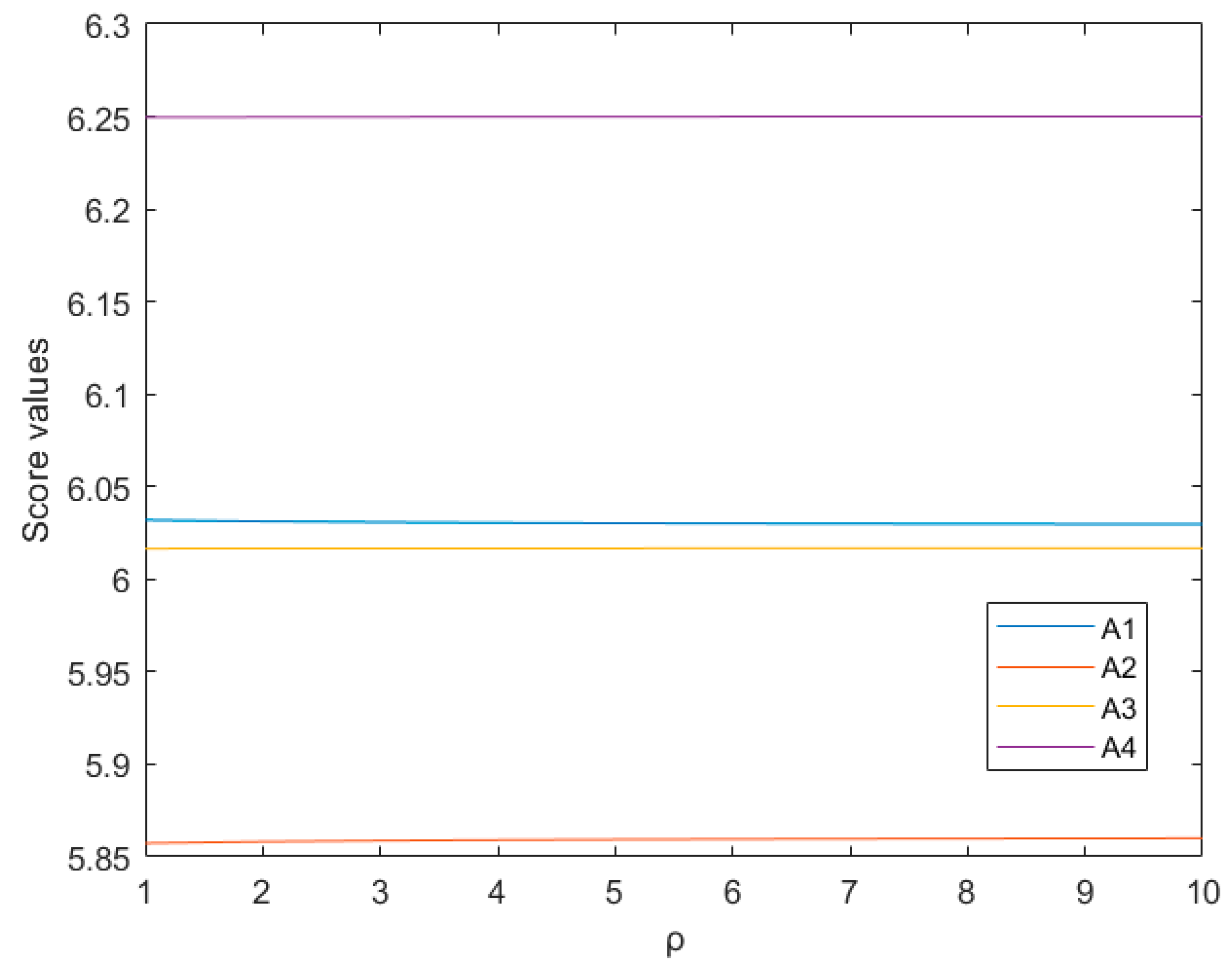
In this section, we investigate the influence of different operational rules on the final decision results. As mentioned above, our method is based on ATT and, when a different generator is used, then different operational rules of alternatives are derived, which reflect the flexibility of our proposed method. Hence, we employ different operational rules of LIBPFNs in the calculation process, and the corresponding score values and ranking orders of alternatives are listed in

Table 6. The score values and ranking orders of alternatives using different operational rules ($\rho =1$).

Operations	Parameters	$\mathbf{Score}\mathbf{Values}\mathit{S}\mathbf{\left(}{\mathbf{\alpha }}_{\mathit{i}}\mathbf{\right)}\mathbf{\left(}\mathit{i}\mathbf{=}\mathbf{1}\mathbf{,}\mathbf{2}\mathbf{,}\mathbf{3}\mathbf{,}\mathbf{4}\mathbf{\right)}$	Ranking Order
Algebraic	None	$S\left({\alpha }_1\right)=s_{5.9654}$$,S\left({\alpha }_2\right)=s_{5.7544}$$,S\left({\alpha }_3\right)=s_{5.9914},$$S\left({\alpha }_4\right)=s_{6.1914}$	$A_4\succ A_3\succ A_1\succ A_2$
Einstein	None	$S\left({\alpha }_1\right)=s_{2.6872}$$,S\left({\alpha }_2\right)=s_{2.2488}$$,S\left({\alpha }_3\right)=s_{2.5336},$$S\left({\alpha }_4\right)=s_{6.1914}$	$A_4\succ A_1\succ A_3\succ A_2$
Hamacher	$\gamma =1$	$S\left({\alpha }_1\right)=s_{2.6657}$$,S\left({\alpha }_2\right)=s_{2.2163}$$,S\left({\alpha }_3\right)=s_{2.4860},$$S\left({\alpha }_4\right)=s_{2.9502}$	$A_4\succ A_1\succ A_3\succ A_2$
Frank	$\delta =2$	$S\left({\alpha }_1\right)=s_{5.9577}$$,S\left({\alpha }_2\right)=s_{5.7459}$$,S\left({\alpha }_3\right)=s_{5.9895},$$S\left({\alpha }_4\right)=s_{6.1829}$	$A_4\succ A_3\succ A_1\succ A_2$
Dombi	$\tau =1$	$S\left({\alpha }_1\right)=s_{6.0320}$$,S\left({\alpha }_2\right)=s_{5.8574}$$,S\left({\alpha }_3\right)=s_{6.0166},$$S\left({\alpha }_4\right)=s_{6.2496}$	$A_4\succ A_1\succ A_3\succ A_2$

.

As seen from Table 6, when a different generator in ATT is employed, i.e., different operational rules for LIVPFNs are used, different score values of alternatives are obtained. In addition, different ranking orders of alternatives are derived. More specifically, when algebraic operational rules are used, the ranking order $A_4\succ A_3\succ A_1\succ A_2$ is produced, and $A_4$ and $A_2$ are the best and worst alternatives. When Einstein operational rules are employed, we can obtain the ranking order $A_4\succ A_1\succ A_3\succ A_2$, and the best and worst alternatives are still $A_4$ and $A_2$. When Hamacher operational rules are used in the calculation process, the ranking order $A_4\succ A_1\succ A_3\succ A_2$ is derived. In addition, when Dombi operational rules of alternatives are used, the same ranking order of alternatives is gained. Finally, when Frank operational rules of LIVPFNs are used, it produces the ranking order $A_4\succ A_3\succ A_1\succ A_2$. Moreover, when different operational rules of LIVPFNs are used, the final ranking orders of alternatives are slightly different, and the best and worst alternatives are always $A_4$ and $A_2$, respectively. In real decision-making problems, DMs can select appropriate operational rules according to actual needs.

6.2.2. The Impact of the Parameter $\rho$ on the Final Decision Results

In this section, we continue to study the influence of the parameter $\rho$ on the final decision results. In this section, we employ Dombi operational rules in the calculation process. We use different values of $\rho$ in the LIVPFAEPWA operator, and the corresponding decision results of alternatives are derived, which is presented as Figure 2.

As it is seen from Figure 2, when different $\rho$ are used in the LIVPFAEPWA operator, then different score values of alternatives are obtained, and the final ranking orders of alternatives are the same, i.e., $A_4\succ A_1\succ A_3\succ A_2$. As a matter of fact, the parameter is a notably important parameter in the EPA operator, as it reflects its strength. As mentioned above, one of the prominent advantages of our proposed AOs is that they can adjust the weights assigned into aggregated LIVPFNs. Hence, DMs can select the appropriate value of $\rho$ according to actual needs.

6.3. Comparative Analysis

In this subsection, we compare our proposed method with some existing ones. First, we compare our method with that developed by Garg [28] based on the LIVPFWA operator. Second, we compare our method with that proposed by Garg and Kumar [39].

6.3.1. Compare with Garg’s [28] Method

Example 3. 

(Revised from [28]). There are three experts,$D_1$,$D_2$, and$D_3$, which are invited to evaluate the five companies$A_1$,$A_2$,$A_3$,$A_4$, and$A_5$for investment. To comprehensively evaluate the performance of the five companies, the four experts evaluate those under four attributes, i.e., the enterprise management level ($C_1$), the business growth ($C_2$), the economic benefit ($C_3$), and the corporate reputation ($C_4$). Weight vectors of attributes and DMs are$w={\left(0.40,0.25,0.20,0.15\right)}^T$and$\lambda ={\left(0.35,0.40,0.25\right)}^T$. Let S = {s₀ = ‘Extremely poor’, s₁ = ‘Very poor’, s₂ = ‘Poor’, s₃ = ‘Slightly poor’, s₄ = ‘Medium’, s₅ = ‘Slightly good’, s₆ = ‘Good’, s₇ = ‘Very good’, s₈ = ‘Extremely good’} be a linguistic term set and DMs employ LIVPFNs to express the evaluation information and three original decision matrices are listed in

Table 7. The decision matrix given by expert $D_1$ in Example 3.

	${\mathit{C}}_1$	${\mathit{C}}_2$	${\mathit{C}}_3$	${\mathit{C}}_4$
$A_1$	$\left(\left[s_2,s_4\right],\left[s_2,s_3\right]\right)$	$\left(\left[s_3,s_5\right],\left[s_2,s_3\right]\right)$	$\left(\left[s_4,s_5\right],\left[s_2,s_3\right]\right)$	$\left(\left[s_2,s_3\right],\left[s_4,s_5\right]\right)$
$A_2$	$\left(\left[s_3,s_4\right],\left[s_3,s_4\right]\right)$	$\left(\left[s_2,s_4\right],\left[s_1,s_2\right]\right)$	$\left(\left[s_1,s_2\right],\left[s_4,s_5\right]\right)$	$\left(\left[s_1,s_3\right],\left[s_4,s_5\right]\right)$
$A_3$	$\left(\left[s_4,s_5\right],\left[s_2,s_3\right]\right)$	$\left(\left[s_2,s_4\right],\left[s_2,s_3\right]\right)$	$\left(\left[s_2,s_4\right],\left[s_1,s_3\right]\right)$	$\left(\left[s_4,s_5\right],\left[s_1,s_3\right]\right)$
$A_4$	$\left(\left[s_4,s_5\right],\left[s_1,s_2\right]\right)$	$\left(\left[s_2,s_3\right],\left[s_2,s_4\right]\right)$	$\left(\left[s_4,s_5\right],\left[s_2,s_3\right]\right)$	$\left(\left[s_3,s_4\right],\left[s_2,s_3\right]\right)$
$A_5$	$\left(\left[s_2,s_3\right],\left[s_1,s_2\right]\right)$	$\left(\left[s_2,s_3\right],\left[s_1,s_3\right]\right)$	$\left(\left[s_3,s_4\right],\left[s_2,s_4\right]\right)$	$\left(\left[s_2,s_3\right],\left[s_3,s_5\right]\right)$

,

Table 8. The decision matrix given by expert $D_2$ in Example 3.

	${\mathit{C}}_1$	${\mathit{C}}_2$	${\mathit{C}}_3$	${\mathit{C}}_4$
$A_1$	$\left(\left[s_2,s_4\right],\left[s_2,s_4\right]\right)$	$\left(\left[s_4,s_5\right],\left[s_2,s_3\right]\right)$	$\left(\left[s_3,s_4\right],\left[s_1,s_3\right]\right)$	$\left(\left[s_2,s_5\right],\left[s_1,s_2\right]\right)$
$A_2$	$\left(\left[s_2,s_5\right],\left[s_2,s_3\right]\right)$	$\left(\left[s_2,s_3\right],\left[s_1,s_4\right]\right)$	$\left(\left[s_1,s_3\right],\left[s_3,s_4\right]\right)$	$\left(\left[s_3,s_6\right],\left[s_1,s_2\right]\right)$
$A_3$	$\left(\left[s_2,s_4\right],\left[s_3,s_4\right]\right)$	$\left(\left[s_5,s_6\right],\left[s_1,s_2\right]\right)$	$\left(\left[s_3,s_5\right],\left[s_2,s_3\right]\right)$	$\left(\left[s_1,s_3\right],\left[s_4,s_5\right]\right)$
$A_4$	$\left(\left[s_5,s_6\right],\left[s_1,s_2\right]\right)$	$\left(\left[s_2,s_3\right],\left[s_3,s_4\right]\right)$	$\left(\left[s_2,s_3\right],\left[s_3,s_4\right]\right)$	$\left(\left[s_2,s_3\right],\left[s_1,s_2\right]\right)$
$A_5$	$\left(\left[s_2,s_4\right],\left[s_2,s_3\right]\right)$	$\left(\left[s_2,s_3\right],\left[s_2,s_4\right]\right)$	$\left(\left[s_3,s_4\right],\left[s_2,s_4\right]\right)$	$\left(\left[s_2,s_3\right],\left[s_4,s_5\right]\right)$

and

Table 9. The decision matrix given by expert $D_3$ in Example 3.

	${\mathit{C}}_1$	${\mathit{C}}_2$	${\mathit{C}}_3$	${\mathit{C}}_4$
$A_1$	$\left(\left[s_2,s_4\right],\left[s_1,s_3\right]\right)$	$\left(\left[s_2,s_3\right],\left[s_2,s_4\right]\right)$	$\left(\left[s_2,s_5\right],\left[s_2,s_3\right]\right)$	$\left(\left[s_4,s_6\right],\left[s_1,s_2\right]\right)$
$A_2$	$\left(\left[s_2,s_4\right],\left[s_2,s_4\right]\right)$	$\left(\left[s_3,s_5\right],\left[s_2,s_3\right]\right)$	$\left(\left[s_3,s_4\right],\left[s_2,s_4\right]\right)$	$\left(\left[s_3,s_4\right],\left[s_2,s_3\right]\right)$
$A_3$	$\left(\left[s_3,s_4\right],\left[s_2,s_3\right]\right)$	$\left(\left[s_4,s_5\right],\left[s_2,s_3\right]\right)$	$\left(\left[s_4,s_5\right],\left[s_1,s_2\right]\right)$	$\left(\left[s_2,s_5\right],\left[s_2,s_3\right]\right)$
$A_4$	$\left(\left[s_1,s_2\right],\left[s_2,s_3\right]\right)$	$\left(\left[s_2,s_3\right],\left[s_2,s_4\right]\right)$	$\left(\left[s_4,s_5\right],\left[s_1,s_2\right]\right)$	$\left(\left[s_3,s_5\right],\left[s_1,s_2\right]\right)$
$A_5$	$\left(\left[s_3,s_4\right],\left[s_2,s_3\right]\right)$	$\left(\left[s_2,s_4\right],\left[s_1,s_2\right]\right)$	$\left(\left[s_1,s_2\right],\left[s_1,s_2\right]\right)$	$\left(\left[s_1,s_3\right],\left[s_4,s_5\right]\right)$

. We use Garg’s [28] method based on the linguistic interval-valued Pythagorean fuzzy weighted average (LIVPFWA) operator and our proposed method based on the LIVPFAEPWA operator to solve Example 3, and the corresponding decision results are listed in

Table 10. The decision results of Example 3 by using different methods.

Decision-Making Methods	$\mathbf{Score}\mathbf{Values}S\mathbf{\left(}{\mathit{\alpha }}_{\mathit{i}}\mathbf{\right)}\mathbf{\left(}\mathit{i}\mathbf{=}\mathbf{1}\mathbf{,}\mathbf{2}\mathbf{,}\mathbf{3}\mathbf{,}\mathbf{4}\mathbf{,}\mathbf{5}\mathbf{\right)}$	Ranking Order
Garg’s [28] method based on the LIVPFWA operator	$S\left({\alpha }_1\right)=s_{6.1152}$$,S\left({\alpha }_2\right)=s_{5.9396}$$,S\left({\alpha }_3\right)=s_{6.2231}$ $S\left({\alpha }_4\right)=s_{6.1832}$$,S\left({\alpha }_5\right)=s_{5.7648}$	$A_3\succ A_4\succ A_1\succ A_2\succ A_5$
Our proposed method based on the LIVPFAEPWA	$S\left({\alpha }_1\right)=s_{6.0108}$$,S\left({\alpha }_2\right)=s_{5.9548}$$,S\left({\alpha }_3\right)=s_{6.1258}$ $S\left({\alpha }_4\right)=s_{6.1232}$$,S\left({\alpha }_5\right)=s_{5.8945}$	$A_3\succ A_4\succ A_1\succ A_2\succ A_5$

.

It is seen from Table 10 that, when different decision-making methods are employed, different score values of alternatives are obtained, and the same ranking order is derived, i.e., $A_3\succ A_4\succ A_1\succ A_2\succ A_5$, which indicates that $A_3$ and $A_4$ are the best and worst alternatives, respectively. However, our proposed method is still more powerful and flexible than Garg’s [28] method. Firstly, Garg’s [28] method is based on the simple algebraic operational rules while our proposed method is based on ATT. As mentioned above, algebraic operational rules are a special case of our proposed operational rules for LIVPFNs. Second, Garg’s [28] method is based on the simple weighted average operator, while our proposed method is based on the EPA operators. It is known that the EPA operator is capable of effectively handling DMs’ extreme or unreasonable evaluation values. In some realistic MAGDM problems, due to many reasons, such as lack of time or expertise, DMs sometimes may provide some unreasonable evaluation values, which obviously negatively affect the final decision results. Hence, it is necessary to reduce the bad influence of DMs’ unreasonable evaluation values. Therefore, our proposed method is more powerful and flexible than that introduced by Garg [28].

6.3.2. Compare with Garg and Kumar’s [39] Method

Example 4. 

(Revised from [39]). Jharkhand is the eastern state of the India. In order to avoid people moving to the urban cities, the Jharkhand government is now considering to establish the industry system based on the agriculture in the rural areas. The government plans to evaluate the potential of four companies and invest in one of them. The four companies are taken as in the form of the alternatives, namely, Surya Food and Agro Pvt. Ltd. ($A_1$), Mother Dairy Fruitand Vegetable Pvt. Ltd. ($A_2$), Parle Products Ltd. ($A_3$), and Heritage Food Ltd. ($A_4$). Three experts ($D_1$,$D_2$, and$D_3$) are invited to evaluate the four companies from four attributes, i.e., project cost ($G_1$), technical capability ($G_2$), financial status ($G_3$), and company background ($G_4$). The weight vector of the four attributes is$w={\left(0.4,0.25,0.2,0.15\right)}^T$. Let S = {s₀ = ‘Extremely poor’, s₁ = ‘Very poor’, s₂ = ‘Poor’, s₃ = ‘Slightly poor’, s₄ = ‘Medium’, s₅ = ‘Slightly good’, s₆ = ‘Good’, s₇ = ‘Very good’, s₈ = ‘Extremely good’} be a linguistic term set and DMs use linguistic interval-valued Atanassov intuitionistic fuzzy numbers (LIVAIFNs) defined on S to express their evaluation information. DMs’ original matrices are listed in

Table 11. The decision matrix given by expert $D_1$ in Example 4.

	${\mathit{C}}_1$	${\mathit{C}}_2$	${\mathit{C}}_3$	${\mathit{C}}_4$
$A_1$	$\left(\left[s_5,s_6\right],\left[s_1,s_2\right]\right)$	$\left(\left[s_4,s_6\right],\left[s_1,s_1\right]\right)$	$\left(\left[s_4,s_5\right],\left[s_2,s_3\right]\right)$	$\left(\left[s_6,s_7\right],\left[s_1,s_1\right]\right)$
$A_2$	$\left(\left[s_3,s_5\right],\left[s_2,s_3\right]\right)$	$\left(\left[s_5,s_6\right],\left[s_1,s_2\right]\right)$	$\left(\left[s_2,s_4\right],\left[s_3,s_4\right]\right)$	$\left(\left[s_3,s_4\right],\left[s_2,s_3\right]\right)$
$A_3$	$\left(\left[s_5,s_6\right],\left[s_1,s_2\right]\right)$	$\left(\left[s_5,s_6\right],\left[s_1,s_2\right]\right)$	$\left(\left[s_3,s_5\right],\left[s_2,s_3\right]\right)$	$\left(\left[s_3,s_5\right],\left[s_1,s_3\right]\right)$
$A_4$	$\left(\left[s_4,s_5\right],\left[s_2,s_3\right]\right)$	$\left(\left[s_1,s_3\right],\left[s_3,s_4\right]\right)$	$\left(\left[s_3,s_5\right],\left[s_1,s_3\right]\right)$	$\left(\left[s_6,s_7\right],\left[s_1,s_1\right]\right)$

,

Table 12. The decision matrix given by expert $D_2$ in Example 4.

	${\mathit{C}}_1$	${\mathit{C}}_2$	${\mathit{C}}_3$	${\mathit{C}}_4$
$A_1$	$\left(\left[s_2,s_4\right],\left[s_1,s_3\right]\right)$	$\left(\left[s_4,s_5\right],\left[s_1,s_2\right]\right)$	$\left(\left[s_4,s_5\right],\left[s_1,s_3\right]\right)$	$\left(\left[s_3,s_6\right],\left[s_1,s_2\right]\right)$
$A_2$	$\left(\left[s_3,s_5\right],\left[s_1,s_3\right]\right)$	$\left(\left[s_1,s_2\right],\left[s_1,s_4\right]\right)$	$\left(\left[s_2,s_3\right],\left[s_3,s_4\right]\right)$	$\left(\left[s_3,s_5\right],\left[s_1,s_3\right]\right)$
$A_3$	$\left(\left[s_3,s_4\right],\left[s_1,s_2\right]\right)$	$\left(\left[s_3,s_6\right],\left[s_1,s_2\right]\right)$	$\left(\left[s_2,s_5\right],\left[s_2,s_3\right]\right)$	$\left(\left[s_3,s_4\right],\left[s_2,s_3\right]\right)$
$A_4$	$\left(\left[s_4,s_5\right],\left[s_1,s_2\right]\right)$	$\left(\left[s_3,s_3\right],\left[s_3,s_5\right]\right)$	$\left(\left[s_3,s_3\right],\left[s_2,s_3\right]\right)$	$\left(\left[s_4,s_6\right],\left[s_1,s_1\right]\right)$

and

Table 13. The decision matrix given by expert $D_3$ in Example 4.

	${\mathit{C}}_1$	${\mathit{C}}_2$	${\mathit{C}}_3$	${\mathit{C}}_4$
$A_1$	$\left(\left[s_2,s_4\right],\left[s_1,s_2\right]\right)$	$\left(\left[s_2,s_3\right],\left[s_1,s_4\right]\right)$	$\left(\left[s_3,s_5\right],\left[s_2,s_3\right]\right)$	$\left(\left[s_5,s_7\right],\left[s_1,s_1\right]\right)$
$A_2$	$\left(\left[s_1,s_4\right],\left[s_2,s_3\right]\right)$	$\left(\left[s_4,s_5\right],\left[s_1,s_2\right]\right)$	$\left(\left[s_2,s_4\right],\left[s_1,s_3\right]\right)$	$\left(\left[s_3,s_4\right],\left[s_2,s_4\right]\right)$
$A_3$	$\left(\left[s_2,s_3\right],\left[s_1,s_5\right]\right)$	$\left(\left[s_3,s_5\right],\left[s_1,s_2\right]\right)$	$\left(\left[s_3,s_5\right],\left[s_1,s_3\right]\right)$	$\left(\left[s_2,s_5\right],\left[s_2,s_3\right]\right)$
$A_4$	$\left(\left[s_3,s_4\right],\left[s_2,s_3\right]\right)$	$\left(\left[s_1,s_2\right],\left[s_3,s_4\right]\right)$	$\left(\left[s_3,s_5\right],\left[s_1,s_2\right]\right)$	$\left(\left[s_5,s_6\right],\left[s_1,s_1\right]\right)$

. The weight vector of DMs is$\lambda ={\left(0.243,0.514,0.243\right)}^T$. We use Garg and Kumar’s [39] method based on the linguistic interval-valued Atanassov intuitionistic fuzzy weighted average (LIVAIFWA) operator and our proposed method based on the LIVPFAEPWA operator to solve Example 4 and present the decision results in

Table 14. The decision results of Example 4 by using different methods.

Decision-Making Methods	$\mathbf{Score}\mathbf{Values}\mathit{S}\left({\mathit{\alpha }}_{\mathit{i}}\right)\left(\mathit{i}=1,2,3,4\right)$	Ranking Order
Garg and Kumar’s [39] method based on a LIVAIFWA operator	$S\left({\alpha }_1\right)=s_{5.1532}$$,S\left({\alpha }_2\right)=s_{4.4817}$$,S\left({\alpha }_3\right)=s_{4.9492}$ $S\left({\alpha }_4\right)=s_{4.5542}$	$A_1\succ A_3\succ A_4\succ A_2$
Our proposed method based on the LIVPFAEPWA	$S\left({\alpha }_1\right)=s_{5.3698}$$,S\left({\alpha }_2\right)=s_{4.3018}$$,S\left({\alpha }_3\right)=s_{4.8661}$ $S\left({\alpha }_4\right)=s_{4.3119}$	$A_1\succ A_3\succ A_4\succ A_2$

.

It is seen from Table 14 that both Garg and Kumar’s [39] and our proposed methods can solve Example 4. Although score values of alternatives obtained by the two methods are different, the ranking orders produced by the two methods are the same i.e., $A_1\succ A_3\succ A_4\succ A_2$, which also indicates the effectiveness of our proposed method. In addition, our proposed method is still more powerful than that developed by Garg and Kumar [39]. First, the application range of our proposed method is much wider than that of Garg and Kumar’s [39]. This is because Garg and Kumar’s [39] method is based on LIVAIFNs, while our method is based on LIVPFNs. As it is known, LIVAIFN is a special case of LIVPFNs. In other word, our method is capable of handling MAGDM problems in which DMs’ preference information is denoted by LIVAIFNs. However, Garg and Kumar’s [39] method is impossible to deal with decision-making problems with LIVPFNs. In addition, Garg and Kumar’s [39] method is based on the simple average operator, and it is powerless to effectively handle DMs’ reasonable evaluation values. Therefore, our proposed method is more powerful and flexible than Garg and Kumar’s [39] method.

7. Conclusions

SBMS is extremely important for modern cement and building industries. As analyzed above, the process of SBMS can be regarded as MAGDM. The main contribution of this paper is to propose a novel MAGDM method and apply it in SBMS. We first introduced some new operational rules for LIVPFNs. The new developed operational laws for LIVPFNs are powerful and flexible, and some special cases are obtained when different t-norms and t-conorms are employed. Moreover, some collections of AOs for LIVPFNs based on EPA and EPG are developed. These operators are capable of capturing the relationship among LIVPFNs, and they can model different MAGDM problems by different parameters and measure diverse correlations among input LIVPFNs by different support functions. In this study, we studied desirable properties of these AOs in detail. Afterwards, based on the new operational rules and AOs, a novel MAGDM method was developed. Last but not least, the new MAGDM method was used to solve an SBMS problem in the cement industry. Parameter analysis showed the flexibility and powerfulness of our method. Comparing analyses demonstrated the advantages and superiorities of our method over some existing ones.

In the future, we shall continue our research from the following aspects. First, in this study, we investigated decision-making problems wherein DMs use LIVPFNs to express their evaluation values. However, in some realistic decision-making problems, DMs would like to use preference relations to express their evaluations, due to many reasons, such as lack of time and expertise. Hence, it is necessary to study preference relations and their applications in decision-making. Similar research has been conducted. For example, Meng et al. [40] generalized LIFSs into linguistic intuitionistic fuzzy preference relations, and studied their desirable properties. In addition, the authors introduced an approach to handle group decision-making problems with incomplete linguistic intuitionistic fuzzy preference relations. Hence, it is necessary and important to propose linguistic interval-valued Pythagorean fuzzy preference relations, investigate their properties, and apply them in decision-making problems. Second, in this study, we assume that DMs are independent. However, in reality, the relationship between DMs and social networks between DMs in decision-making situations has received scholars’ attention. In [41,42,43,44], scholars studied social networks-based group decision-making methods in IFSs, hesitant fuzzy sets, Pythagorean fuzzy sets, hesitant fuzzy linguistic term sets, etc. Hence, in the future, we shall study social network-based decision-making methods under LIVPFSs. Finally, our study does not consider the consensus levels of DMs. As matter of fact, considering the importance of consensus in group decision-making, more and more scholars have focused on group decision-making methods by considering the consensus reaching process [45,46,47,48,49]. Therefore, in the future, we will study group decision-making methods.

References

1. Akadiri, P.O.; Olomolaiye, P.O.; Chinyio, E.A. Multi-criteria evaluation model for the selection of sustainable materials for building projects. Autom. Constr. 2013, 30, 113–125. [Google Scholar] [CrossRef]
2. Mahmoudkelaye, S.; Azari, K.T.; Pourvaziri, M.; Asadian, E. Sustainable material selection for building enclosure through ANP method. Case Stud. Constr. Mater. 2018, 9, e00200. [Google Scholar] [CrossRef]
3. Roy, J.; Das, S.; Kar, S.; Pamucar, D. An extension of the CODAS approach using interval-valued intuitionistic fuzzy set for sustainable material selection in construction projects with incomplete weight information. Symmetry 2019, 11, 393. [Google Scholar] [CrossRef] [Green Version]
4. Meng, F.Y.; Dong, B.H. Linguistic intuitionistic fuzzy PROMETHEE method based on similarity measure for the selection of sustainable building materials. J. Ambient Intel. Hum. Comp. 2022, 13, 4415–4435. [Google Scholar] [CrossRef]
5. Chen, Z.S.; Martinez, L.; Chang, J.P.; Wang, X.J.; Xiong, S.H.; Chin, K.S. Sustainable building material selection: A QFD-and ELECTRE III-embedded hybrid MCGDM approach with consensus building. Eng. Appl. Artif. Intel. 2019, 85, 783–807. [Google Scholar] [CrossRef]
6. Khoshnava, S.M.; Rostami, R.; Valipour, A.; Ismail, M.; Rahmat, A.R. Rank of green building material criteria based on the three pillars of sustainability using the hybrid multi criteria decision making method. J. Clean. Prod. 2018, 173, 82–99. [Google Scholar] [CrossRef]
7. Ahmed, M.; Qureshi, M.N.; Mallick, J.; Ben Kahla, N. Selection of sustainable supplementary concrete materials using OSM-AHP-TOPSIS approach. Adv. Mater. Sci. Eng. 2019, 2019, 2850480. [Google Scholar] [CrossRef] [Green Version]
8. Chen, Z.S.; Yang, L.L.; Chin, K.S.; Yang, Y.; Pedrycz, W.; Chang, J.P.; Martínez, L.; Skibniewski, M.J. Sustainable building material selection: An integrated multi-criteria large group decision making framework. Appl. Soft Comput. 2021, 113, 107903. [Google Scholar] [CrossRef]
9. Siksnelyte-Butkiene, I.; Streimikiene, D.; Balezentis, T.; Skulskis, V. A systematic literature review of multi-criteria decision-making methods for sustainable selection of insulation materials in buildings. Sustainability 2021, 13, 737. [Google Scholar] [CrossRef]
10. Mukherjee, I.; Singh, U.K.; Chakma, S. Evaluation of groundwater quality for irrigation water supply using multi-criteria decision-making techniques and GIS in an agroeconomic tract of Lower Ganga basin, India. J. Environ. Manag. 2022, 309, 114691. [Google Scholar] [CrossRef]
11. Sajjad, M.; Sałabun, W.; Faizi, S.; Ismail, M.; Watrobski, J. Statistical and analytical approach of multi-criteria group decision-making based on the correlation coefficient under intuitionistic 2-tuple fuzzy linguistic environment. Expert Syst. Appl. 2022, 193, 116341. [Google Scholar] [CrossRef]
12. Li, Z.Y.; Zhang, X.Y.; Wang, W.J.; Li, Z. Multi-criteria probabilistic dual hesitant fuzzy group decision making for supply chain finance credit risk assessments. Expert Syst. 2022, 39, e13015. [Google Scholar] [CrossRef]
13. Haseena, S.; Saroja, S.; Revathi, T. A fuzzy approach for multi criteria decision making in diet plan ranking system using cuckoo optimization. Neural Comput. Appl. 2022, 34, 13625–13638. [Google Scholar] [CrossRef]
14. Tian, C.; Peng, J.J.; Long, Q.Q.; Wang, J.Q.; Goh, M. Extended picture fuzzy MULTIMOORA method based on prospect theory for medical institution selection. Cogn. Comput. 2022, 14, 1446–1463. [Google Scholar] [CrossRef]
15. Zadeh, L.A. The concept of a linguistic variable and its application to approximate reasoning—I. Inf. Sci. 1975, 8, 199–249. [Google Scholar] [CrossRef]
16. Zadeh, L.A. The concept of a linguistic variable and its application to approximate reasoning—II. Inf. Sci. 1975, 8, 301–357. [Google Scholar] [CrossRef]
17. Atanassov, K.T. Intuitionistic fuzzy sets. Fuzzy Sets Syst. 1986, 20, 87–96. [Google Scholar] [CrossRef]
18. Yager, R.R. Pythagorean membership grades in multicriteria decision making. IEEE Trans. Fuzzy Syst. 2014, 22, 958–965. [Google Scholar] [CrossRef]
19. Zhang, H. Linguistic intuitionistic fuzzy sets and application in MAGDM. J. Appl. Math. 2014, 2014, 432092. [Google Scholar] [CrossRef] [Green Version]
20. Garg, H. Linguistic Pythagorean fuzzy sets and its applications in multiattribute decision-making process. Int. J. Intell. Syst. 2018, 33, 1234–1263. [Google Scholar] [CrossRef]
21. Sarkar, B.; Biswas, A. Linguistic Einstein aggregation operator-based TOPSIS for multicriteria group decision making in linguistic Pythagorean fuzzy environment. Int. J. Intell. Syst. 2021, 36, 2825–2864. [Google Scholar] [CrossRef]
22. Lin, M.W.; Wei, J.C.; Xu, Z.S.; Chen, R.Q. Multiattribute group decision-making based on linguistic Pythagorean fuzzy interaction partitioned Bonferroni mean aggregation operators. Complexity 2018, 2018, 9531064. [Google Scholar] [CrossRef] [Green Version]
23. Lin, M.W.; Huang, C.; Xu, Z.S. TOPSIS method based on correlation coefficient and entropy measure for linguistic Pythagorean fuzzy sets and its application to multiple attribute decision making. Complexity 2019, 2019, 6967390. [Google Scholar] [CrossRef]
24. Ping, Y.J.; Liu, R.; Wang, Z.L.; Liu, H.C. New approach for quality function deployment with an extended alternative queuing method under linguistic Pythagorean fuzzy environment. Eur. J. Ind. Eng. 2022, 16, 349–370. [Google Scholar] [CrossRef]
25. Han, Q.; Li, W.M.; Lu, Y.L.; Zheng, M.F.; Quan, W.; Song, Y.F. TOPSIS method based on novel entropy and distance measure for linguistic Pythagorean fuzzy sets with their application in multiple attribute decision making. IEEE Access 2019, 8, 14401–14412. [Google Scholar] [CrossRef]
26. Liu, H.C.; Quan, M.Y.; Li, Z.W.; Wang, Z.L. A new integrated MCDM model for sustainable supplier selection under interval-valued intuitionistic uncertain linguistic environment. Inf. Sci. 2019, 486, 254–270. [Google Scholar] [CrossRef]
27. Mu, Z.M.; Zeng, S.Z.; Wang, P.Y. Novel approach to multi-attribute group decision-making based on interval-valued Pythagorean fuzzy power Maclaurin symmetric mean operator. Comput. Ind. Eng. 2021, 155, 107049. [Google Scholar] [CrossRef]
28. Garg, H. Linguistic interval-valued Pythagorean fuzzy sets and their application to multiple attribute group decision-making process. Cogn. Comput. 2020, 12, 1313–1337. [Google Scholar] [CrossRef]
29. Beliakov, G.; Pradera, A.; Calvo, T. Aggregation Functions: A Guide for Practitioners; Springer: Berlin/Heidelberg, Germany; New York, NY, USA, 2007. [Google Scholar]
30. Wang, L.; Garg, H. Algorithm for multiple attribute decision-making with interactive Archimedean norm operations under Pythagorean fuzzy uncertainty. Int. J. Comput. Intell. Syst. 2021, 14, 503–527. [Google Scholar] [CrossRef]
31. Qin, Y.C.; Qi, Q.F.; Shi, P.Z.; Scott, P.J.; Jiang, X.Q. Linguistic interval-valued intuitionistic fuzzy Archimedean prioritised aggregation operators for multi-criteria decision making. J. Intell. Fuzzy Syst. 2020, 38, 4643–4666. [Google Scholar] [CrossRef]
32. Yager, R.R. The power average operator. IEEE Trans. Syst. Man Cybern.-Part A 2001, 31, 724–731. [Google Scholar] [CrossRef]
33. Xu, Z.S.; Yager, R.R. Power geometric operators and their use in group decision making. IEEE Trans. Fuzzy Syst. 2009, 18, 94–105. [Google Scholar]
34. Xu, Z.S. Approaches to multiple attribute group decision making based on intuitionistic fuzzy power aggregation operators. Knowl.-Based Syst. 2011, 24, 749–760. [Google Scholar] [CrossRef]
35. He, Y.D.; He, Z.; Wang, G.D.; Chen, H.Y. Hesitant fuzzy power Bonferroni means and their application to multiple attribute decision making. IEEE Trans. Fuzzy Syst. 2014, 23, 1655–1668. [Google Scholar] [CrossRef]
36. Xiong, S.H.; Chen, Z.S.; Chang, J.P.; Chin, K.S. On extended power average operators for decision-making: A case study in emergency response plan selection of civil aviation. Comput. Ind. Eng. 2019, 130, 258–271. [Google Scholar] [CrossRef]
37. Li, L.; Ji, C.; Wang, J. A novel multi-attribute group decision-making method based on q-rung dual hesitant fuzzy information and extended power average operators. Cogn. Comput. 2021, 13, 1345–1362. [Google Scholar] [CrossRef]
38. Klir, G.J.; Yuan, B. Fuzzy Sets and Fuzzy Logic; Prenticehall: Hoboken, NJ, USA, 1995. [Google Scholar]
39. Meng, F.Y.; Tang, J.; Fujita, H. Linguistic intuitionistic fuzzy preference relations and their application to multi-criteria decision making. Inf. Fusion 2019, 46, 77–90. [Google Scholar] [CrossRef]
40. Garg, H.; Kumar, K. Linguistic interval-valued Atanassov intuitionistic fuzzy sets and their applications to group decision making problems. IEEE Trans. Fuzzy. Syst. 2019, 27, 2302–2311. [Google Scholar] [CrossRef]
41. Pei, F.; He, Y.W.; Yan, A.; Zhou, M.; Chen, Y.W.; Wu, J. A consensus model for intuitionistic fuzzy group decision-making problems based on the construction and propagation of trust/distrust relationships in social networks. Int. J. Fuzzy Syst. 2020, 22, 2664–2679. [Google Scholar] [CrossRef]
42. Chen, H.P. Hesitant fuzzy multi-attribute group decision making method based on weighted power operators in social network and their application. J. Intell. Fuzzy Syst. 2021, 40, 9383–9401. [Google Scholar] [CrossRef]
43. Liu, Y.; Diao, W.X.; Yang, J.; Yi, J.H. A visual social network group consensus approach with minimum adjustment based on Pythagorean fuzzy set. Iran. J. Fuzzy Syst. 2021, 18, 167–183. [Google Scholar]
44. Ren, R.X.; Tang, M.; Liao, H.C. Managing minority opinions in micro-grid planning by a social network analysis-based large scale group decision making method with hesitant fuzzy linguistic information. Knowl.-Based Syst. 2020, 189, 105060. [Google Scholar] [CrossRef]
45. Li, Y.H.; Kou, G.; Li, G.X.; Peng, Y. Consensus reaching process in large-scale group decision making based on bounded confidence and social network. Eur. J. Oper. Res. 2022, 303, 790–802. [Google Scholar] [CrossRef]
46. Gai, T.T.; Cao, M.S.; Chiclana, F.; Wu, J.; Laing, C.Y.; Herrera-Viedma, E. A decentralized feedback mechanism with compromise behavior for large-scale group consensus reaching process with application in smart logistics supplier selection. Expert Syst. Appl. 2022, 204, 117547. [Google Scholar] [CrossRef]
47. Zha, Q.B.; Cai, J.F.; Gu, J.P.; Liu, G.W. Information learning-driven consensus reaching process in group decision-making with bounded rationality and imperfect information: China’s urban renewal negotiation. Appl. Intell. 2022. [Google Scholar] [CrossRef]
48. Li, Z.L.; Zhang, Z.; Yu, W.Y. Consensus reaching with consistency control in group decision making with incomplete hesitant fuzzy linguistic preference relations. Comput. Ind. Eng. 2022, 170, 108311. [Google Scholar] [CrossRef]
49. Zha, Q.B.; Dong, Y.C.; Chiclana, F.; Herrera-Viedma, E. Consensus reaching in multiple attribute group decision making: A multi-stage optimization feedback mechanism with individual bounded confidences. IEEE Trans. Fuzzy Syst. 2022, 30, 3333–3346. [Google Scholar] [CrossRef]
Figure 1. The flowchart of our proposed MAGDM method.
Sustainability 15 00106 g001
Figure 2. Score values of A i when τ = 1 , ρ [ 1 ,   10 ] .
Sustainability 15 00106 g002