Abstract
This paper develops a multi-objective mixed-integer linear programming model for the problem of robust rescheduling for capacitated urban rail transit (URT) trains to serve passengers from delayed high-speed railway (HSR) trains. The capacity of each extra train is not assumed to be unlimited in this paper. Robust passenger assignment constraints are developed to ensure that delayed passengers can board the URT trains under different random delay scenarios of HSR operations. Robust dispatching constraints of URT trains are designed for a stable disrupting number of URT trains across different scenarios. The multi-objective model is used to maximize the number of expected transported passengers and minimize the number of extra trains and operation-ending time of all extra trains. An iterative solution approach based on a revised version of the epsilon-constraint method combined with the weighted-sum method is designed for the computation of the multi-objective model. Computational experiments are performed on the Beijing URT lines and the Beijing-Shanghai HSR line. We evaluate the impact of the robustness constraints of passenger assignment and the number of extra trains to ensure that the number of trains are maintained and the passengers can successfully take the trains during different delayed scenarios.
1. Introduction
Urban rail transit (URT) lines are typically connected with high speed-railway (HSR) lines at hub transfer stations to provide transfer services for passengers. The URT system is of crucial importance for the urban transportation system to meet the transportation demands of passengers from HSR trains, especially when there are fewer buses and taxis operated late at night. For instance, HSR passengers prefer taking URT trains at Beijing South Railway Station since it always takes more than one hour to wait for a taxi, and it is inconvenient to take buses at night.
Inevitably unplanned events such as adverse weather conditions, rolling stock break-down, signal problems, or infrastructure failures often occur during HSR operations. HSR trains will arrive at the transfer stations very late and miss the last URT trains if the disruptions occur late at night. Therefore, rescheduling URT trains to serve delayed passengers is very meaningful and challenging, especially when disruptions occur during HSR operations under an uncertain and stochastic environment. Considering delays under an uncertain environment leads to forms of robust timetabling [1]. There are numerous studies that focus on designing a robust timetable in the train timetabling stage. The robust timetable could accommodate uncertainties unfolding in real-time dispatching [2,3,4,5,6,7,8,9,10,11,12,13,14]. Furthermore, the robust dispatching timetables could provide a robust train meet-pass sequence [8] or a stable train routing [12]. However, a limited number of researchers considered designing a robust rescheduling timetable from the perspective of passengers and operating companies [15].
This paper studies the problem of Robust Rescheduling for Capacitated URT trains (RRCU) to serve passengers from delayed HSR trains late at night. We consider studying the robustness of the assigning of delayed passengers and the dispatching of URT trains. It should be noted that the disruption occurs during HSR operations instead of the URT operations. Moreover, the disruption occurs with an uncertain duration, which results in a series of different arrival times of HSR trains at their destination. We formulate robust “scheduling policies” of the URT system, corresponding to a series of reactive decisions under uncertain predicated operational conditions of the HSR system with probabilistic data input.
In daily operation, the dispatchers of the URT system always consider the following four typical train dispatching measures to serve delayed passengers: (1) rescheduling the train timetable by adjusting arrival and departure times at passing stations; (2) adjusting the train stopping pattern; (3) adjusting the train routing; and (4) running extra trains. Although some studies in the literature [16,17] begin to study this problem, most dispatchers still currently make these decisions manually on the basis of their experiences and professional judgments, which is typically in lacking in rigorous computation and optimization [18]. In this paper, we consider developing a mathematically rigorous optimization model that could be solved using commercial solvers such as CPLEX. Besides this, we consider running extra trains as the primary scheduling policy, and hereby we define extra trains as trains that operate in emergency cases and later than the last train on the same URT line.
This paper develops a mixed-integer linear programming model to solve the problem of RRCU. In our model, the capacity of each extra train is not assumed to be unlimited since there are many passengers from delayed HSR trains at transfer stations. A robust passenger assignment constraint is developed to ensure that delayed passengers board the URT trains under different random delay scenarios of HSR operations. Robust dispatching constraints of URT trains guarantee that URT dispatchers implement rescheduling timetables smoothly with the uncertain arrival time of delayed HSR trains at transfer stations. Furthermore, both the objectives of delayed passengers and of URT operators need to be identified and described when disruption occurs under an uncertain and stochastic environment late at night. The resulting multi-objective optimization problem is to maximize the expected transported passengers and minimize the number of extra trains and operation-ending time of all extra trains. Three objectives mutually influence and restrict each other. Therefore, an iterative approach based on a revised version of the epsilon-constraint method combined with the weighted-sum method is designed for the computation of the multi-objective model.
The remainder of this paper proceeds as follows. In Section 2, a detailed literature review on the Train Timetable Rescheduling (TTR) problem and Timetable Synchronization Problem (TSP) is presented. In Section 3, a problem statement and model assumptions are given first, which are followed by a multi-objective model that formalizes the problem of RRCU. Then, we designed an iterative approach based on a revised version of the epsilon-constraint method combined with the weighted-sum method for the computation of the multi-objection model. Numerical experiments based on the Beijing-Shanghai (Jing-Hu) High-Speed Railway (HSR) line and Beijing Urban Rail Transit (URT) lines are given in Section 4 to evaluate the performance and effectiveness of the bi-objective model. We conclude this paper in Section 5.
2. Literature Review
The problem of Robust Rescheduling for Capacitated Urban rail transit trains (RRCU) is a Train Timetable Rescheduling (TTR) problem. It is also a Timetable Synchronization Problem (TSP), since we need to synchronize the timetables of Urban Rail Transit trains (URT) trains to serve delayed passengers of High-Speed Railway (HSR) trains when disruption occurs during HSR operations. In this section, we review state of the art for two directions: (1) Train Timetable Rescheduling (TTR) problem; (2) Timetable Synchronization Problem (TSP).
The Train Timetable Rescheduling (TTR) problem has been well studied in the past few decades. The TTR problem is viewed as a huge job shop scheduling problem with no-store constraints by D’Ariano et al. [19]. They used a combination of a job shop and an alternative graph model to solve the TTR problem. Corman et al. [20] employed the alternative graph to reschedule trains with different classes of priority. Schöbel [21] considered the convenience of all passengers and presented a path-based and activity-based linear programming model to minimize the average delay of a passenger when arriving at their destination. Recently, the TTR problem in an uncertain and stochastic environment has been studied by some researchers. For example, Meng et al. [8] proposed a rescheduling model to minimize the expected additional delay under different forecasted operational conditions, where uncertain segment running times, segment recovery times, and the possibilities of rescheduling decisions are considered. Meng et al. [12] proposed an integer programming model based on the cumulative flow variables for dispatching trains in a stochastic environment. They introduced stable train routing constraints to ensure that trains traverse on the same route under different capacity scenarios. Some review papers [13,22,23] present detailed information about the real-time TTR problem.
There are some trade-offs among the objectives of each subsystem during the real-time train rescheduling. For example, dispatchers want to recover the initial timetable as soon as possible and minimize the total deviation time of all trains involved. While passengers expect to arrive at their destination with shorter waiting times and travel times, operating companies want trains to run in order and have the lowest operating expense. Corman et al. [24] used a detailed alternative graph model to solve the rescheduling problem while considering the needs of dispatchers and passengers. The resulting bi-objective problem is supposed to minimize train delays and missed connections. Two heuristic algorithms are developed to obtain the Pareto front of the bi-objective problem. Luan et al. [25] have proposed a mixed-integer linear programming model to formalize the inequity of competitors and represent the competing relationship of multiple train operating companies. A model is further reformulated with the objective of maximizing the individual deviation of competitors’ delay cost from the average delay cost to provide a more flexible framework.
Many researchers have studied timetable synchronization for regional or national rail transit systems. On the one hand, many researchers have studied timetable synchronization during peak hours [26,27,28,29,30,31,32,33,34,35,36,37,38], in which the primary focus is to minimize the inconvenience of passengers who must transfer between different lines at transfer stations. On the other hand, researchers [39,40,41,42,43,44] who have studied timetable synchronization during late-night operation are concerned with network accessibility, since passengers may fail to transfer after operation has ended at some connected lines.
As shown above, although a variety of studies have focused on the Train Timetable Rescheduling (TTR) problem and the Timetable Synchronization Problem (TSP), the problem of rescheduling URT trains to serve passengers from delayed HSR trains is still neglected. Moreover, few researchers [1,8,10,11,12,13,44,45,46] pay attention to the uncertain and stochastic factors of real-world operations in rescheduling the timetable.
This paper aims to offer the following contributions:
- We present a rigorous mixed-integer programming model to solve the problem of robust rescheduling for capacitated URT trains, in which multiple scenarios are used to represent the uncertainty of arrival time at destinations of delayed HSR trains. The robust passenger assignment constraint is introduced to ensure the decision robustness of passenger assignment under different scenarios. Finally, the robust dispatching constraint is designed for the stable disrupting number of URT trains across different scenarios.
- We consider both objectives of delayed passengers and URT operators in the model. The resulting multi-objective optimization problem is to maximize the expected transported passengers and minimize the number of extra trains and operation-ending time of all extra trains.
- We design a novel iterative solution approach based on a revised version of the epsilon-constraint method combined with the weighted-sum method, which is designed for the computation of the multi-objective model.
3. Mathematical Formulation
3.1. Problem Statement
The inputs of the problem include:
- A High-Speed Railway (HSR) line and Urban Rail Transit (URT) lines
A network including an HSR line and URT lines is given as some lines and stations. Clearly, one HSR line and two URT lines are shown in the illustrative network Figure 1.
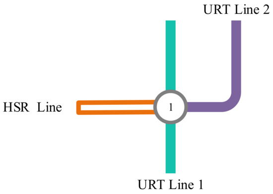
Figure 1.
An illustrative network.
- 2.
- A set of extra trains of the URT system
For each extra train, we know its origin and destination stations, the free-flow running time between two adjacent stations, the stopping pattern, the minimum and maximum dwell time at intermediate stations, and the passenger carrying capacity.
- 3.
- A set of delayed HSR trains with uncertain delay information
For each delayed HSR train, we know its uncertain characteristic of arrival time at the destination station and passenger carrying volume.
Three objectives are considered for optimization: maximize the expected transported passengers of delayed HSR train, minimize the number of extra trains, and minimize the operation-ending time of all extra trains.
The problem includes the following three key decisions, based on which a detailed timetable of extra URT trains as the major output can be obtained.
- For each URT lines, we need to determine the number of extra trains that operate on it.
- For each extra URT train, we need to determine the departure time at the first station, the arrival time at the last station, the arrival and departure time at the intermediate stations, and the headway between two adjacent trains in the same line.
- For passengers of the delayed train, we need to determine which parts of it transfer to which extra train.
In our model, we make the following assumptions:
- We do not consider passenger transfer activities between URT trains.
- The rescheduling for the rolling stock plan of URT system is neglected.
- The passenger transfer walking time at the transfer station is known and fixed.
- In each station, passengers will always ride the first arriving train after they reach the platform to reduce their waiting time [40].
- We do not consider the train rescheduling of HSR system.
3.2. Formulation of the Multi-Objective Model
In Table 1, Table 2 and Table 3, we introduce the notation that will be used to define our model. The tables contain, in order, general subscripts, input parameters, and decision variables.

Table 1.
General subscripts.
Table 2.
Input parameters.
Table 3.
Decision variables.
3.2.1. Objective Functions
The problem of Robust Rescheduling for Capacitated URT trains (RRCU) requires an optimization from the viewpoint of the delayed passengers and URT operating company. On the one hand, we model the objective function of delayed passengers as the maximization of the expected transported passengers of delayed HSR trains. This objective function can be formulated as follows:
On the other hand, the operating company prefers to operate fewer extra trains to reduce operating expenses and finish operation earlier for vehicle cleaning and maintenance. As a result, we formulate the URT operating company’s objectives as the minimization of the number of extra URT trains and the operation-ending time of all extra trains. The objective functions can be formulated as follows:
3.2.2. Constraints
This section describes the constraints for the problem of Robust Rescheduling for Capacitated URT trains (RRCU).
- Start time constraints at the origin station:
Constraints (4) specify that the routing of each extra train must start from its origin node after its predetermined earliest start time.
- Departure time constraints:
Constraints (5) define that the departure time of each extra train at intermediate station is equal to the sum of its arrival time and dwell time at station .
- Arrival time constraints:
Constraints (6) specify that the arrival time of each extra train at station is more than or equal to the sum of its departure time at station and travel time from station to station .
- Headway time constraints at origin station
Constraints (7) define the headway time between two adjacent trains. Constraints (8) make sure that the headway time is more than or equal to the minimum headway time.
- Minimum and maximum dwell time constraints at the intermediate station:
Constraints (9) specify that the dwell time of each extra train at intermediate station is more (less) than or equal to its minimum (maximum) planned dwell time. Specifically, the difference between the minimum and maximum planned dwell times is more than 0 only if there is a scheduled stop in the timetable for extra train at station .
- Dwell time constraints of two adjacent trains:
Constraints (10) ensure the equal dwell time of two adjacent trains on the same line.
Train connection time constraints:
Constraints (11) define the train connection time by the departure time of connecting extra train, the arrival time of feeder train, and the walking time from feeder line to connecting line at transfer station .
- Transfer direction constraints:
Constraints (12) specify the transfer direction of delayed passengers. Recall that is the probability of passengers from train being assigned to extra train . is the subscript of and indicates a transfer direction from line (i.e., HSR line) to (i.e., the URT line which operates extra train ). It should be noted that we need to distinguish the direction of the URT lines, since some URT lines are bi-directional. Constraints (12) guarantee that the number of delayed passengers from train who are assigned to the connecting train and following train is less than or equal to the passengers who could be assigned to the transfer direction to .
- Passenger flow balance constraints:
Constraints (13) require that the total number of passengers assigned to the connected trains be less than or equal to the volume of impacted passengers
- Train capacity constraints:
Constraints (14) guarantee that the passenger carrying capacity of each connected train is not violated.
- Mapping constraints between passenger assignment and extra train passenger assignment constraints:
Constraints (15) and (16) are imposed on mapping the passenger assignment variable to the extra train passenger assignment variable . Constraints (15) and (16) represent the following if-then constraints:
- Mapping constraints between transfer connection time and extra train connection constraints:
Constraints (17) and (18) are imposed on mapping the connection time variable to the extra train connection variable . Constraints (17) and (18) represent the following if-then constraints:
- Extra train constraints:
Constraints (19) and (20) are imposed on mapping the extra train passenger assignment variable and extra train connection variable to extra train operation variable . will be equal to1 if and only if and were both equal to 1, otherwise, will be 0. The if-then constraints are as follows:
- Mapping constraints between passenger assignment and extra train operation constraints:
Constraints (22) and (23) are imposed on mapping the extra train operation variable to passenger assignment variable . Constraints (22) and (23) represent the following if-then constraints:
- Robust passenger assignment constraints:
Constraints (24) ensure that the number of passengers of delayed train assigned to the train is identical under different random scenarios.
- Robust train rescheduling constraints:
Constraints (25) ensure that the operational situations of each extra train are identical under different random scenarios. Constraints (24) and (25) impose the robustness of passenger assignment and the number of extra trains for the rescheduling timetables.
- Passenger assignment constraints:
Constraints (26) and (27) impose the order of the passenger assignment and extra train operation between two adjacent trains.
3.3. Solution Approach of the Multi-Objective Model
This section describes an iterative approach of the -constraint method combined with the weighted-sum method for the computation of a multi-objection model as illustrated in Section 3.1 and Section 3.2.
D’Ariano et al. [1] proposed an iterative procedure based on the “weighted-sum” or “-constraint” approach to solve the model with two objectives. Inspired by their research, we design an iterative procedure based on the -constraint method combined with the weighted-sum method to solve the proposed multi-objective model. The multi-objective function is separated into two parts by the -constraint method: one is a bi-objective function of the expected transported passengers and operation-ending time of all extra trains of Urban Rail Transit (URT) system, another one is a single-objective function of the number of extra URT trains. The weighted-sum method is designed to solve the bi-objective function. The method is achieved using two input parameters and as the weights of the two objectives, respectively, defined by the decision maker. The following conditions followed: .
Algorithm 1 illustrates the steps of the iterative procedure. Recall that , , and is the objective of the expected transported passengers, number of extra URT trains, and the operation-ending time of all extra trains, respectively. We let , , and be the value of the solution for the problem of robust rescheduling for capacitated URT trains with max , min , and min , respectively. In addition, we let () be the value of () for the optimal solution with the objective function max . Additionally, we define as the value of the performance indicator regarding the optimal solution of the problem with max at iteration .
The iterative procedure is based on three steps: Step One is the initialized phase, Step Two is the iterative phase, and Step Three filters the solutions in .
| Algorithm 1 The solution approach for the multi-objective model |
| Input: |
| Begin |
| Step 1: Initialization, set |
| 1.1 max subject to constraints (4) –(27), and set |
| 1.2 min subject to constraints (4) –(27), and set |
| 1.3 min subject to constraints (4) –(27), and set , . is the lower bound as well as is the upper bound of objective. We vary the from to , and set the iteration interval as |
| 1.4 set , , |
| 1.5 max subject to constraints (4) –(27), and set , |
| 1.6 insert the pair in the set of solution values |
| Step 2: while do |
| Begin |
| 2.1 Set |
| 2.2 max subjective to Constraints (4)–(28) plus constraint: , |
| 2.3 set , |
| 2.4 insert the pair in the set of solution values |
| End |
| Step 3: return the non-dominated pairs from the set of |
| End |
Regarding the fractional steps in Step One, Steps 1.1 and 1.2 are required for the computation of and ; Step 1.3 is used to obtain , the lower and upper bound of the objective. We could vary the values or and repeat Steps 1.4, 1.5, and 1.6 to search for new compromise solutions. Once the decision makers give a fixed value of or , the two objective functions of and will be a single objective function by weighted-sum function . Thanks to this revised weighted-sum method, we only need to solve a model with one objective at each iteration in Step 2.
Step Two is the iterative phase; at each iteration, we solve a single-objective formulation, and performance indicators of the expected transported passengers and the operation-ending time of all extra trains are directly optimized in the objective function .
4. Numerical Experiments
To test how well the models may be applied in the real-world network, we performed numerical experiments using operational data from the Beijing-Shanghai (Jing-Hu) High-Speed Railway (HSR) line and Beijing Urban Rail Transit (URT) lines. The experiments are performed with reasonable assumptions: (1) The delay time of all HSR trains arriving at their destination is identical under the same scenario; (2) the loading rate of each HSR train is known from the HSR operating company. Before reporting the experimental results, we describe the dataset in Section 4.1. We adopt the CPLEX solver version 12.3 with default settings to solve the model. The following experiments are all performed on a computer Intel(R) Core(TM) i7-4770 CPU @ 3.40 GHz processor and 4 GB RAM.
4.1. Test Case Description
- Network data:
Figure 2 shows the network that consists of 44 stations and 3 lines (i.e., the Jing-Hu HSR line, lines 4 and 14 of the Beijing URT system). Lines 4 and 14 of the Beijing URT system connect with the Jing-Hu HSR line at Beijing South Railway Station (BSRS) for passengers transferring.
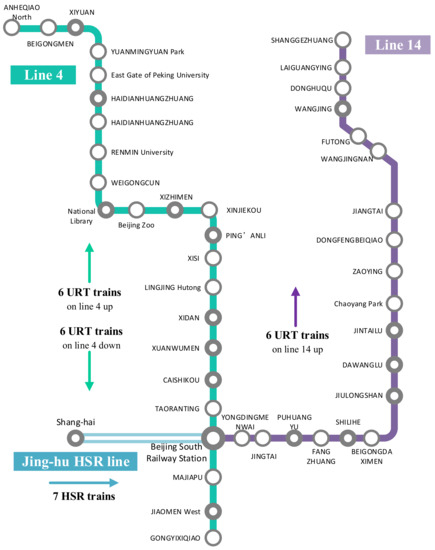
Figure 2.
The studied network.
- URT trains data:
The free-flow running time and passenger-carrying capacity of trains that operate on the same line are identical. Figure 3 illustrates the free-flow running time of a URT train on lines 4 and 14. The capacity of trains on lines 4 and 14 are 1480 and 1960 (unit: person), respectively.
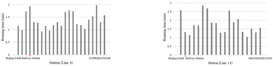
Figure 3.
The free-flow running time of URT trains between two adjacent stations. (* is the hub).
- Delayed HSR trains data:
Seven HSR trains of Jing-Hu HSR line are considered: G150, G152, G18, G154, G44, G22, and G158. Table 4 illustrates the planned arrival time and passenger carrying volume of delayed trains.
Table 4.
Planned arrival time and passenger carrying volume of HSR trains.
The delayed time arriving at destinations of each HSR trains is subject to a Weibull distribution as shown in Figure 4. We consider ten delay scenarios of the arrival delays following a 2-parameter Weibull distribution, as illustrated in Table 5. The following parameters in the form of [scale, shape] are used as scale = 15.2248 and shape = 1.30277. These values of arrival delay time come from fitting to the real-life data of the Jing-hu HSR line from September to December in 2017.
where is the delayed time of scenario , is the scale parameter, and is the shape parameter of the distribution. is the cumulative distribution function for the Weibull distribution.
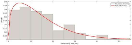
Figure 4.
Weibull distribution of delayed time arriving at destinations of HSR trains.
Table 5.
Delayed time and occurrence probability of ten scenarios.
4.2. Performance Evaluation of Single-Objective Model
We use the Jing-Hu HSR line and lines 4 and 14 of the Beijing URT system in Figure 5 as the test bed, considering several instances with different numbers of URT trains in order to assess the performance of the proposed model and the influence of the number of URT trains considered to be the objective of expected transported passengers of delayed HSR trains. We here range the numbers of URT trains from 3 to 18, a subset of the 18 trains described in Figure 2. The objective function used in this section is as followed:
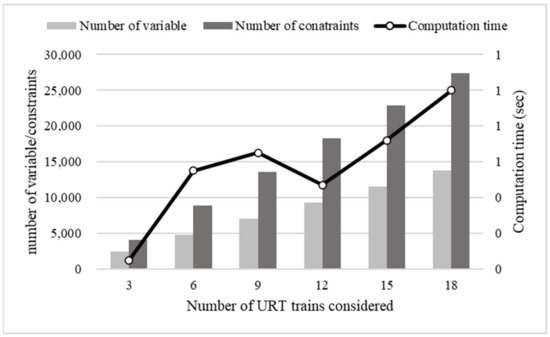
Figure 5.
Number of variables, constraints, and computational time.
In this section, we only focus on the maximization of expected transported passengers of delayed HSR trains and neglect minimizing number of extra trains and total operation-ending time. The bars indicate the number of variables or constraints in Figure 5 and refer to the Y-axis on the left-hand side. The lines (with symbols) indicate computation time in Figure 5 and refer to the Y-axis on the right-hand side. As listed in Table 6 and shown in Figure 5, the number of variables and constraints increases with the increasing number of URT trains considered. Since the computational time of 6 experiments is less than 1 s, we conclude that the solver can quickly solve the model, and the analysis on the computational time can be ignored in the following experiments.
Table 6.
Number of variables, constraints, computational time, and optimal solutions of three objectives.
We report the optimal solutions of three objectives in Table 6 and Figure 6. Recall that , , and are the objective functions of the expected transported passengers, the number of extra URT trains, and the operation-ending time of all extra trains, respectively. We define to be the value of the optimal solution of the single-objective model with max . Additionally, we define () as the value of the performance indicator () regarding the optimal solution of the single objective with max . The bars indicate optimal values for the objective of expected transported passengers in Figure 6a, the number of extra URT trains in Figure 6b, and the operation-ending time in Figure 6c, respectively.
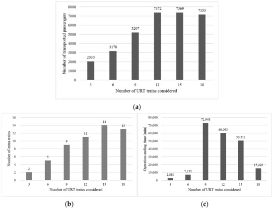
Figure 6.
Optimal solutions of three objectives. (a) Expected transported passengers (), (b) Number of extra URT trains ( ), (c) Operation-ending time of all extra trains ( ).
We can see that the optimal values of operation-ending time and the number of extra trains increase with an increase in the number of URT trains considered (when the number of URT trains considered is less than 15). The number of transported passengers increases when the number of URT trains considered is less than 12. In Section 4.3 and Section 4.4, further experiments will be performed in the instances with 12 URT trains considered that are solved to optimality in a short computational time.
4.3. Search for Pareto-Optimal Solutions
4.3.1. Parameter Analysis of the Weighted-Sum Method
This section studies the multi-objective problem, for instance (Table 6), with URT trains. We tested several settings of for the iterative approach. Recall that two objective functions of the expected transported passengers () and the operation-ending time of all extra trains () will be a single objective function by using the weighted-sum method with a fixed value on or .
We now study the influences of different values of on the optimal values. The value of is proportional to the value of , which is the weight for the objective . At each iteration, the optimal value increases with an increase in the value of , as illustrated in Figure 7. The bars indicate optimal values of the function (i.e., objectives of expected transported passengers and operation-ending time) and refer to the Y-axis on the left-hand side. The lines (with symbols) indicate optimal values for the objective of the number of extra trains in Figure 7 and refer to the Y-axis on the right-hand side.
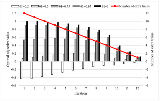
Figure 7.
Results of the parameter analysis experiments.
We conclude that the optimal values are better when the weight for the objective of expected transported passengers () is increased. Overall, the objective of the expected transported passengers is more important than the objective of the operation-ending time of all extra trains in the RRCU problem.
4.3.2. Results of the Pareto-Optimal Solutions
This section studies the experimental results of the iterative approach by varying the upper bound (ranging from 1 to 12) of the objective of with the fixed value of and . The surface with symbols in Figure 8 indicates the Pareto frontier. The instance generated by the iterative approach based on a revised version of the -constraint method combined with the weighted-sum method is quick to solve, since this iterative approach treats the multi-objective problem as an iterative single-objective optimization problem.
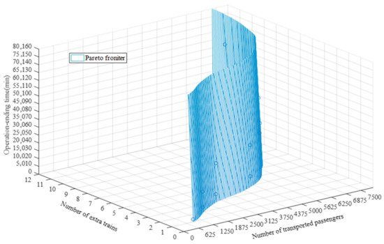
Figure 8.
Pareto frontier.
4.3.3. Further Analysis of the Experimental Results of the Single-Objective Model and Multi-Objective Model
Recall that three objectives are considered as maximizing expected transported passengers , minimizing the number of extra URT trains , and minimizing the operation-ending time of all extra trains in the multi-objective model. The single-objective model focuses on the maximization of expected transported passengers and neglects minimizing the number of extra trains and total operation-ending time. We report the values of three objectives obtained by single-objective and multi-objective models in Figure 9. The bars indicate the expected transported passengers in Figure 9a and operation-ending time in Figure 9b, respectively, and refer to the Y-axis. The values of the objective of the number of extra trains are reported in the X-axis in Figure 9a,b.
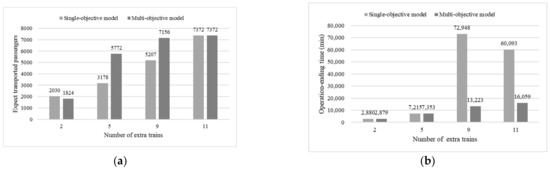
Figure 9.
Results of the single-objective model and multi-objective model (), (a) Objectives of expected transported passengers and number of extra URT trains, (b) Objectives of operation-ending time and number of extra URT trains.
Regarding the objective of expected transported passengers in Figure 9a, the multi-objective model performs better than the single-objective when we fixed the value of . This is because we considered minimizing the number of extra trains in the multi-objective model and neglected it in the single-objective model. A similar reason leads to the values of objective obtained by the multi-objective model being less than the values obtained by the single-objective model in Figure 9b. In summary, the multi-objective model is better than the single-objective model for solving the problem of robust rescheduling for capacitated URT trains, and is the optimal solution with more expected transported passengers, a smaller number of extra trains, and less operation-ending time.
4.4. Impact of Uncertainty towards Robustness
This section presents computational results on the stochastic modeling environment in stochastic optimization. The value of is 0.5 for four cases.
- WAR: Iterative approach with robustness consideration of both passenger assignment and number of extra trains.
- WPR: Iterative approach with robustness consideration of passenger assignment solutions and without robustness consideration of the number of extra trains.
- WER: Iterative approach with robustness consideration of the number of extra trains and without robustness consideration of passenger assignment solutions.
- NAR: Iterative approach without robustness consideration of both passenger assignment and number of extra trains.
Table 7 shows the critical characteristic of the robust case studies. Recall that ten scenarios of the arrival delays of each HSR train at its destination station are considered. The constraints (24) guarantee an identical number of transported passengers under different random scenarios, which lead to the robustness of passenger assignment. Constraints (25) ensure that the operational situations of each extra train are identical under different random scenarios.
Table 7.
Essential characteristic of the robust case studies.
Analysis of the Experimental Results of Four Cases
Figure 10 illustrates the results of case WAR, WPR, WER, and NAR. The bars indicate the optimal objective value and refer to the Y-axis on the left-hand side; the line (with symbols) indicates the gap of optimal objective value between WAR and NAR and refers to the Y-axis on the right-hand side. Figure 10 does not show the gap of the optimal objective value between WAR, WPR, WER, and NAR, for the optimal objective values of WAR, WPR, and WER are identical at each iteration.
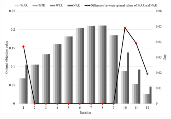
Figure 10.
Experimental results of WAR, WPR, WTR, and NAR.
We now study the reason why the optimal objective values of WAR, WPR, and WER are identical at each iteration. Recall that constraints (24) are and is the passenger assignment variables, meaning the number of passengers from delayed train that are assigned to the extra connecting train under scenario . Constraints (25) are , and is the extra train operation variables, which indicate if train operates on line under scenario . Constraints (15), (16), (19), and (20) imposed that the extra train operation variable is if the passenger assignment variable is .
Constraints (22) and (23) are imposed on mapping the extra train operation variable to the passenger assignment variable . If , the is more than 0, which corresponds with the number of passengers from delayed train that are assigned to the extra connecting train under scenario . In summary, constraints (24) and (25) are mutual restraint by constraints (15), (16), (19), (20), (22), and (23).
Figure 11 illustrates the optimal values for the objective of the number of extra URT trains. As shown, the value of the number of extra URT trains is identical for iteration 2 to 12 as a linear decrement function of the iteration. The reason why it is a linear decrement function is that we use the -constraint method to set the upper bound of as , in which , as illustrated in Step 2.2 in Algorithm 1, and we set at each iteration.
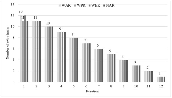
Figure 11.
Number of extra trains () of WAR, WPR, WTR, and NAR.
Regarding the optimal solution quality as shown in Figure 10 and Figure 11, the NAR approach yields the best performance since its range is maximum among four cases. The reason why its range is maximum is that it does not consider the robustness of both passenger assignment and the number of extra trains. From the results of Figure 10 and Figure 11, we conclude that the WPR, WTR, and WAR approaches have the same performances at every iteration. A robust rescheduling solution obtained by the WPR, WTR, and WAR approaches is better than NAR for passengers and dispatchers in reality.
5. Conclusions and Future Research
This paper investigated the mathematical models and methods for managing a multi-objective problem of practical interest for railway managers who have to reschedule Urban Rail Transit (URT) trains to serve passengers from delayed High-Speed Railway (HSR) trains. We presented a mixed-integer linear programming model to address this problem, in which the capacity of each extra train is not assumed to be unlimited. A robust passenger assignment constraint is introduced to ensure the decision robustness of passenger assignment under different scenarios, and a robust dispatching constraint is designed for the stable disrupting number of URT trains across different scenarios. Three objectives are to maximize the number of expected transported passengers, minimize the number of extra trains, and minimize the operation-ending time of all extra trains. An iterative approach based on a revised version of the -constraint method combined with the weighted-sum method is designed for the computation of a multi-objective model.
Computational experiments on Beijing URT lines and the Beijing-Shanghai HSR line show that the proposed methodology could be applied in real-world operations. First, our method could be used to identify Pareto optimal solutions, measuring the performance of the proposed model and the influence of the number of extra trains considered against the three objectives. Then, the model could find a trade-off between the indicators of three objectives. Besides this, we evaluate the impact of the robustness constraints of passenger assignment and the number of extra trains among the different delayed scenarios.
Our future work will address the following research directions: Passenger ODs should be considered in the model to study which lines of the URT system need to run extra trains. The rolling stock rescheduling of extra trains could be developed to achieve a lower operating expense of the URT system.
Author Contributions
Data curation, Y.B.; Formal analysis, S.L.; Methodology, S.L; Software, Y.B.; Writing—review & editing, W.W. All authors have read and agreed to the published version of the manuscript.
Funding
This work was funded by a project from Science and Technology Research and Development Program of the China National Railway Group Limited grant number [P2021S012], National Natural Science Foundation of China grant number [71571012, 61790573]. And The APC was funded by [P2021S012].
Institutional Review Board Statement
Not applicable.
Informed Consent Statement
Not applicable.
Data Availability Statement
Some or all data, models, or code that support the findings of this study are available from the corresponding author upon reasonable request.
Acknowledgments
The generous assistance of Francesco Corman from ETH Zurich, Shuge Yao and Xiaofeng Chai from Beijing Jiaotong University are greatly appreciated. The authors are of course responsible for all results and opinions expressed in this paper.
Conflicts of Interest
The authors declare no conflict of interest.
References
- D’Ariano, A.; Meng, L.; Centulio, G.; Corman, F. Integrated stochastic optimization approaches for tactical scheduling of trains and railway infrastructure maintenance. Comput. Ind. Eng. 2019, 127, 1315–1335. [Google Scholar] [CrossRef]
- Carey, M.; Kwieciński, A. Stochastic approximation to the effects of headways on knock-on delays of trains. Transp. Res. Part B Methodol. 1994, 28, 251–267. [Google Scholar] [CrossRef]
- Carey, M. Optimizing scheduled times, allowing for behavioural response. Transp. Res. Part B Methodol. 1998, 32, 329–342. [Google Scholar] [CrossRef]
- Zhou, X.; Khan, M.B. Slack time allocation in robust double-track train timetabling applications. IEEE Trans. Intell. Transp. Syst. 2010, 11, 81–89. [Google Scholar]
- Shafia, M.A.; Aghaee, M.P.; Sadjadi, S.J.; Jamili, A. Robust Train Timetabling Problem: Mathematical Model and Branch and Bound Algorithm. IEEE Trans. Intell. Transp. Syst. 2011, 13, 307–317. [Google Scholar] [CrossRef]
- Bešinović, N.; Goverde, R.M.; Quaglietta, E.; Roberti, R. An integrated micro–macro approach to robust railway timetabling. Transp. Res. Part B Methodol. 2016, 87, 14–32. [Google Scholar] [CrossRef] [Green Version]
- Burggraeve, S.; Bull, S.H.; Vansteenwegen, P.; Lusby, R.M. Integrating robust timetabling in line plan optimization for railway systems. Transp. Res. Part C Emerg. Technol. 2017, 77, 134–160. [Google Scholar] [CrossRef] [Green Version]
- Meng, L.; Zhou, X. Robust single-track train dispatching model under a dynamic and stochastic environment: A scenario-based rolling horizon solution approach. Transp. Res. Part B: Methodol. 2011, 45, 1080–1102. [Google Scholar] [CrossRef]
- Cacchiani, V.; Toth, P. Nominal and robust train timetabling problems. Eur. J. Oper. Res. 2012, 219, 727–737. [Google Scholar] [CrossRef]
- Quaglietta, E.; Corman, F.; Goverde, R.M. Stability of railway dispatching solutions under a stochastic and dynamic environment. In Proceedings of the RailCopenhagen2013: 5th International Seminar on Railway Operations Modelling and Analysis (IAROR), Copenhagen, Denmark, 13–15 May 2013; Institute for Transport Planning and Systems, ETH Zurich: Zurich, Switzerland, 2013. [Google Scholar]
- Larsen, R.; Pranzo, M.; D’Ariano, A.; Corman, F.; Pacciarelli, D. Susceptibility of optimal train schedules to stochastic disturbances of process times. Flex. Serv. Manuf. J. 2014, 26, 466–489. [Google Scholar] [CrossRef]
- Meng, L.; Luan, X.; Zhou, X. A train dispatching model under a stochastic environment: Stable train routing constraints and reformulation. Netw. Spat. Econ. 2016, 16, 791–820. [Google Scholar] [CrossRef]
- Cavone, G.; Dotoli, M.; Epicoco, N.; Seatzu, C. A decision making procedure for robust train rescheduling based on mixed integer linear programming and Data Envelopment Analysis. Appl. Math. Model. 2017, 52, 255–273. [Google Scholar] [CrossRef]
- Hong, X.; Meng, L.; Corman, F.; D’Ariano, A.; Veelenturf, L.P.; Long, S. Robust Capacitated Train Rescheduling with Passenger Reassignment under Stochastic Disruptions. Transp. Res. Rec. J. Transp. Res. Board 2021, 2675, 214–232. [Google Scholar] [CrossRef]
- Long, S.; Meng, L.; Miao, J.; Hong, X.; Corman, F. Synchronizing Last Trains of Urban Rail Transit System to Better Serve Passengers from Late Night Trains of High-Speed Railway Lines. Networks Spat. Econ. 2020, 20, 599–633. [Google Scholar] [CrossRef]
- Cacchiani, V.; Huisman, D.; Kidd, M.; Kroon, L.; Toth, P.; Veelenturf, L.; Wagenaar, J. An overview of recovery models and algorithms for real-time railway rescheduling. Transp. Res. Part B Methodol. 2014, 63, 15–37. [Google Scholar] [CrossRef] [Green Version]
- Corman, F.; D’Ariano, A.; Pacciarelli, D.; Pranzo, M. Optimal inter-area coordination of train rescheduling decisions. Transp. Res. Part E Logist. Transp. Rev. 2012, 48, 71–88. [Google Scholar] [CrossRef] [Green Version]
- Yin, J.; Tang, T.; Yang, L.; Gao, Z.; Ran, B. Energy-efficient metro train rescheduling with uncertain time-variant passenger demands: An approximate dynamic programming approach. Transp. Res. Part B Methodol. 2016, 91, 178–210. [Google Scholar] [CrossRef]
- D’Ariano, A.; Pacciarelli, D.; Pranzo, M. A branch and bound algorithm for scheduling trains in a railway network. Eur. J. Oper. Res. 2007, 183, 643–657. [Google Scholar] [CrossRef]
- Corman, F.; D’Ariano, A.; Hansen, I.A.; Pacciarelli, D. Optimal multi-class rescheduling of railway traffic. J. Rail Transp. Plan. Manag. 2011, 1, 14–24. [Google Scholar] [CrossRef]
- Schöbel, A. Integer programming approaches for solving the delay management problem. In Algorithmic Methods for Railway Optimization; Springer: Berlin/Heidelberg, Germany, 2007; pp. 145–170. [Google Scholar]
- Fang, W.; Yang, S.; Yao, X. A survey on problem models and solution approaches to rescheduling in railway networks. IEEE Trans. Intell. Transp. Syst. 2015, 16, 2997–3016. [Google Scholar] [CrossRef]
- Corman, F.; Meng, L. A Review of Online Dynamic Models and Algorithms for Railway Traffic Management. IEEE Trans. Intell. Transp. Syst. 2014, 16, 1274–1284. [Google Scholar] [CrossRef]
- Corman, F.; D’Ariano, A.; Pacciarelli, D.; Pranzo, M. Bi-objective conflict detection and resolution in railway traffic management. Transp. Res. Part C Emerg. Technol. 2012, 20, 79–94. [Google Scholar] [CrossRef]
- Luan, X.; Corman, F.; Meng, L. Non-discriminatory train dispatching in a rail transport market with multiple competing and collaborative train operating companies. Transp. Res. Part C Emerg. Technol. 2017, 80, 148–174. [Google Scholar] [CrossRef]
- Goverde, R. Transfer Stations and Synchronization; Delft University of Technology: Delft, The Netherlands, 1999. [Google Scholar]
- Daduna, J.R.; Voß, S. Practical experiences in schedule synchronization. In Computer-Aided Transit Scheduling; Springer: Berlin/Heidelberg, Germany, 1995; pp. 39–55. [Google Scholar]
- Domschke, W. Schedule synchronization for public transit networks. Oper.-Res.-Spektrum 1989, 11, 17–24. [Google Scholar] [CrossRef]
- Ceder, A.; Tal, O. Timetable synchronization for buses. In Computer-Aided Transit Scheduling; Springer: Berlin/Heidelberg, Germany, 1999; pp. 245–258. [Google Scholar]
- Nachtigall, K. Periodic network optimization with different arc frequencies. Discret. Appl. Math. 1996, 69, 1–17. [Google Scholar] [CrossRef] [Green Version]
- Odijk, M.A. A constraint generation algorithm for the construction of periodic railway timetables. Transp. Res. Part B Methodol. 1996, 30, 455–464. [Google Scholar] [CrossRef]
- Zwaneveld, P.J.; Kroon, L.G.; Romeijn, H.E.; Salomon, M.; Dauzère-Pérès, S.; Van Hoesel, S.P.M.; Ambergen, H.W. Routing Trains Through Railway Stations: Model Formulation and Algorithms. Transp. Sci. 1996, 30, 181–194. [Google Scholar] [CrossRef] [Green Version]
- Kroon, L.G.; Romeijn, H.E.; Zwaneveld, P.J. Routing trains through railway stations: Complexity issues. Eur. J. Oper. Res. 1997, 98, 485–498. [Google Scholar] [CrossRef] [Green Version]
- Wong, R.C.W.; Yuen, T.W.Y.; Fung, K.W.; Leung, J.M.Y. Optimizing Timetable Synchronization for Rail Mass Transit. Transp. Sci. 2008, 42, 57–69. [Google Scholar] [CrossRef]
- Shafahi, Y.; Khani, A. A practical model for transfer optimization in a transit network: Model formulations and solutions. Transp. Res. Part A Policy Pr. 2010, 44, 377–389. [Google Scholar] [CrossRef]
- Cevallos, F.; Zhao, F. Minimizing transfer times in public transit network with genetic algorithm. Transp. Res. Rec. 2006, 1971, 74–79. [Google Scholar] [CrossRef]
- Chen, C.H.; Yan, S.; Tseng, C.H. Inter-city bus scheduling for allied carriers. Transportmetrica 2010, 6, 161–185. [Google Scholar] [CrossRef]
- Yan, F.; Goverde, R.M. Combined line planning and train timetabling for strongly heterogeneous railway lines with direct connections. Transp. Res. Part B Methodol. 2019, 127, 20–46. [Google Scholar] [CrossRef]
- Zhou, W.; Deng, L.; Xie, M.; Yang, X. Coordination optimization of the first and last trains’ departure time on urban rail transit network. Adv. Mech. Eng. 2013, 5, 848292. [Google Scholar] [CrossRef]
- Kang, L.; Zhu, X.; Wu, J.; Sun, H.; Siriya, S.; Kanokvate, T. Departure time optimization of last trains in subway networks: Mean-variance model and GSA algorithm. J. Comput. Civ. Eng. 2015, 29, 04014081. [Google Scholar] [CrossRef]
- Kang, L.; Wu, J.; Sun, H.; Zhu, X.; Gao, Z. A case study on the coordination of last trains for the Beijing subway network. Transp. Res. Part B Methodol. 2015, 72, 112–127. [Google Scholar] [CrossRef]
- Kang, L.; Wu, J.; Sun, H.; Zhu, X.; Wang, B. A practical model for last train rescheduling with train delay in urban railway transit networks. Omega 2015, 50, 29–42. [Google Scholar] [CrossRef]
- Li, W.; Xu, R.; Luo, Q.; Jones, S. Coordination of last train transfers using automated fare collection (AFC) system data. J. Adv. Transp. 2016, 50, 2209–2225. [Google Scholar] [CrossRef]
- Yang, S.; Yang, K.; Gao, Z.; Yang, L.; Shi, J. Last-Train Timetabling under Transfer Demand Uncertainty: Mean-Variance Model and Heuristic Solution. J. Adv. Transp. 2017, 2017, 5095021. [Google Scholar] [CrossRef] [Green Version]
- Li, X.; Yang, X. A stochastic timetable optimization model in subway systems. Int. J. Uncertain. Fuzziness Knowl.-Based Syst. 2013, 21 (Suppl. S1), 1–15. [Google Scholar] [CrossRef]
- Wu, Y.; Tang, J.; Yu, Y.; Pan, Z. A stochastic optimization model for transit network timetable design to mitigate the randomness of traveling time by adding slack time. Transp. Res. Part C Emerg. Technol. 2015, 52, 15–31. [Google Scholar] [CrossRef]
Publisher’s Note: MDPI stays neutral with regard to jurisdictional claims in published maps and institutional affiliations. |
© 2022 by the authors. Licensee MDPI, Basel, Switzerland. This article is an open access article distributed under the terms and conditions of the Creative Commons Attribution (CC BY) license (https://creativecommons.org/licenses/by/4.0/).