Stacking Model for Photovoltaic-Power-Generation Prediction

Abstract

Despite the clean and renewable advantages of solar energy, the instability of photovoltaic power generation limits its wide applicability. In order to ensure stable power-grid operations and the safe dispatching of the power grid, it is necessary to develop a model that can accurately predict the photovoltaic power generation. As a widely used prediction method, the stacking model has been applied in many fields. However, few studies have used stacking models to predict photovoltaic power generation. In the research, we develop four different stacking models that are based on extreme gradient boosting, random forest, light gradient boosting, and gradient boosting decision tree to predict photovoltaic power generation, by using two datasets. The results show that the prediction accuracy of the stacking model is higher than that of the single ensemble-learning model, and that the prediction accuracy of the Stacking-GBDT model is higher than the other stacking models. The stacking model that is proposed in this research provides a reference for the accurate prediction of photovoltaic power generation.

1. Introduction

With the increasing shortage of nonrenewable energy, environmental pollution is becoming more and more serious, and the development of renewable energy is becoming a common goal. As one of the countries with the highest carbon emissions in the world, China aims to peak its carbon emissions by 2030, and to become carbon neutral by 2060. China will continue to further optimize its energy structure and gradually improve the safe, efficient, clean, and low-carbon modern-energy-source system, and it will achieve carbon peak and carbon neutrality according to the established goals. As the main substitute for fossil energy, solar energy plays a very important strategic role in carbon-emission reduction. With the gradually increasing attention to solar energy resources, photovoltaic power generation (PV generation) has been vigorously promoted, and its scale has been expanding. Photovoltaic energy is becoming an important basic energy in social production and in life. According to the United Nations Madrid Climate Change Conference on China’s 2050 photovoltaic development outlook, China will soon enter the period of the large-scale and accelerated deployment of photovoltaic energy; by 2050, photovoltaic energy will become the largest power source in China, and it will account for about 40 percent of the country’s electricity consumption that year [1]. However, meteorological factors, such as temperature and humidity, fluctuate greatly with time and show intermittent and random characteristics, which lead to constant fluctuations in the photovoltaic power generation and bring challenges to the operation of the power-supply system. Therefore, the prediction of photovoltaic power generation remains an important and challenging research field.

According to the time range, photovoltaic predictions can be divided into four types: very-short-term predictions, short-term predictions, medium-term predictions, and long-term predictions [2]. Dimd et al. (2022) defined the prediction range of the min–hour as very-short-term prediction, the hour–week as short-term prediction, the day–month as medium-term prediction, and the month–year as long-term prediction [2]. In order to develop an energy policy according to future photovoltaic energy generation, the government mainly pays attention to the long-term prediction. In order to prepare a power-production plan, to control power reserves, and to evaluate purchase and sales contracts, electric power enterprises mainly carry out short-term or very-short-term predictions. In this research, we propose a short-term forecasting model from the perspective of enterprises.

There are two types of prediction methods: traditional forecasting methods and machine-learning methods. The traditional prediction methods mainly include linear regression (LR) [3], auto-regression (AR) [4], regression moving average with exogenous variables (ARMAX) [5,6], and others. These traditional methods are mostly based on linear relationships and they have limited abilities to reflect nonlinear relationships. The relationship between the power generation and the influencing factors is mostly nonlinear. Machine learning is different from traditional statistical methods in that it does not have strict requirements on data distribution, it can deal with high-dimensional data, and dimension reduction is easy. Thanks to the development of machine-learning methods and the availability of photovoltaic-power-generation data and meteorological data, data-based machine-learning methods have become more and more popular in the field of photovoltaic forecasting [7,8,9,10,11,12,13,14,15]. However, most studies use a single machine-learning model, and the generalization and the robustness of this research are not sufficient. In recent years, researchers have developed different ensemble-learning algorithms, including bagging, boosting, and stacking. On the basis of the above three algorithms, scholars developed three models: the bagging model, the boosting model, and the stacking model [16,17,18]. The stacking model differs from the bagging and boosting models in two main ways. Firstly, the stacking model usually considers heterogeneous weak learners (different learning algorithms are combined together), while bagging and boosting mainly consider homogeneous weak learners. Secondly, the stacking model combines base models with the meta-model, while bagging and boosting combine weak learners according to deterministic algorithms. In this study, we attempt to develop four stacking models. More than three years of data from Australia, as well as data from a Chinese photovoltaic power station, were used in this study. Although there have been studies that use ensemble-learning-based models to predict the photovoltaic power generation, our study is quite different from theirs. Lee et al. (2020) compared the prediction performances of different ensemble-learning-based models, while we constructed stacking models on the basis of different ensemble-learning-based models and compared the prediction performances of different stacking models [14]. Some scholars have also used stacking models to predict the photovoltaic power generation [19,20], in which only the results of the first layer were taken as the input of the second layer. We not only take the results of the first layer as the input of the second layer, but we also consider the input data of the first layer comprehensively. In addition, the previous authors built only one stacking model, while we built different stacking models and compared their predictive performances, which is one of the main contributions of this paper.

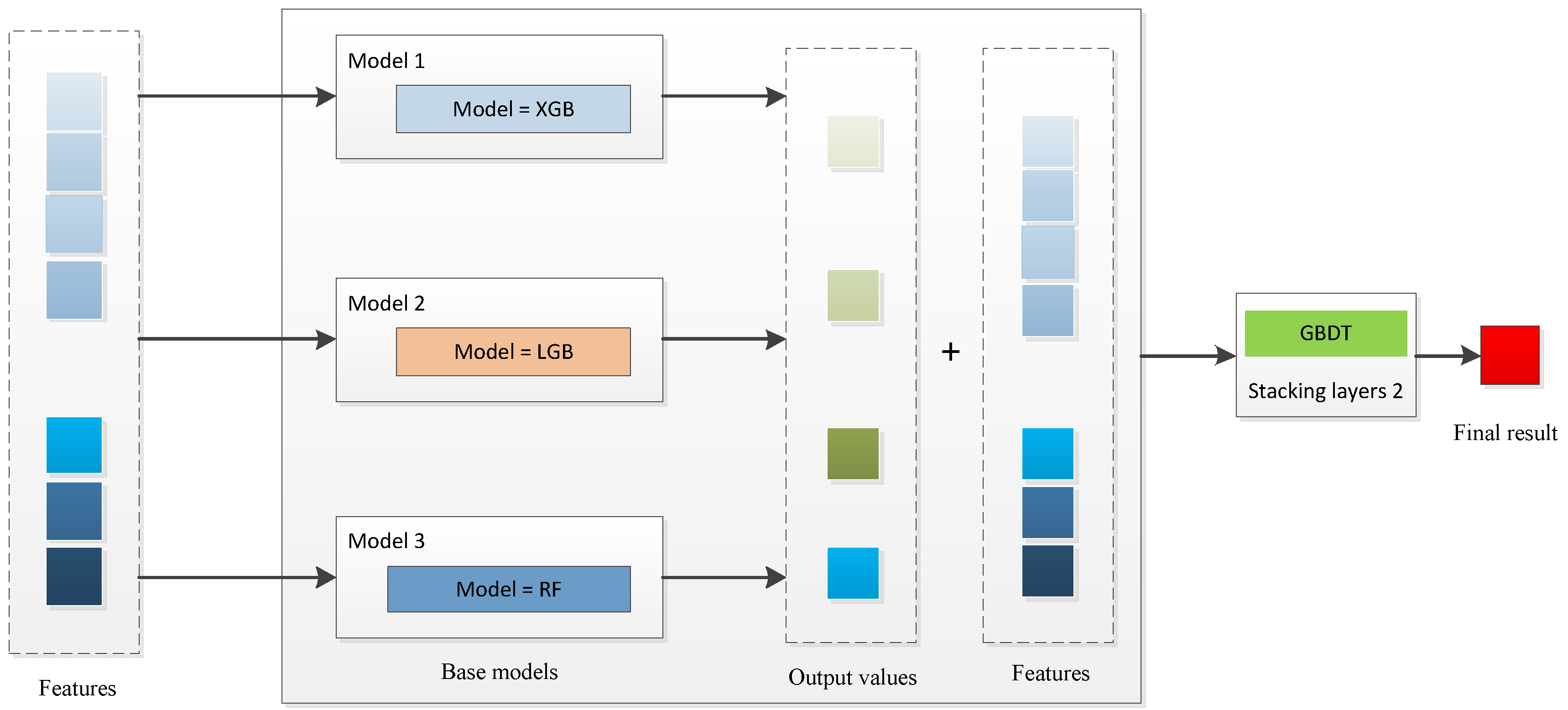
The contributions of this paper are as follows. (1) The first innovation was to propose a stacking model that is based on different ensemble algorithms (XGB, RF, GBDT, and LGB). We not only take the results of the first layer as the input of the second layer, but we also consider the input data of the first layer comprehensively. This is the first stacking model to predict photovoltaic power generation by using different ensemble algorithms, and by considering the input data and the output results of the first layer comprehensively. (2) The second innovative idea of this paper was to determine which stack model has the best predictive performance. As far as we know, this research is the first to systematically develop and compare the application of four different stacking models to the prediction of photovoltaic power generation. (3) Previous studies mainly used a single data source; however, this study used Australian panel and Chinese cross-sectional data. A comparative analysis of the various data not only verifies the robustness of the model, but also demonstrates its universality.

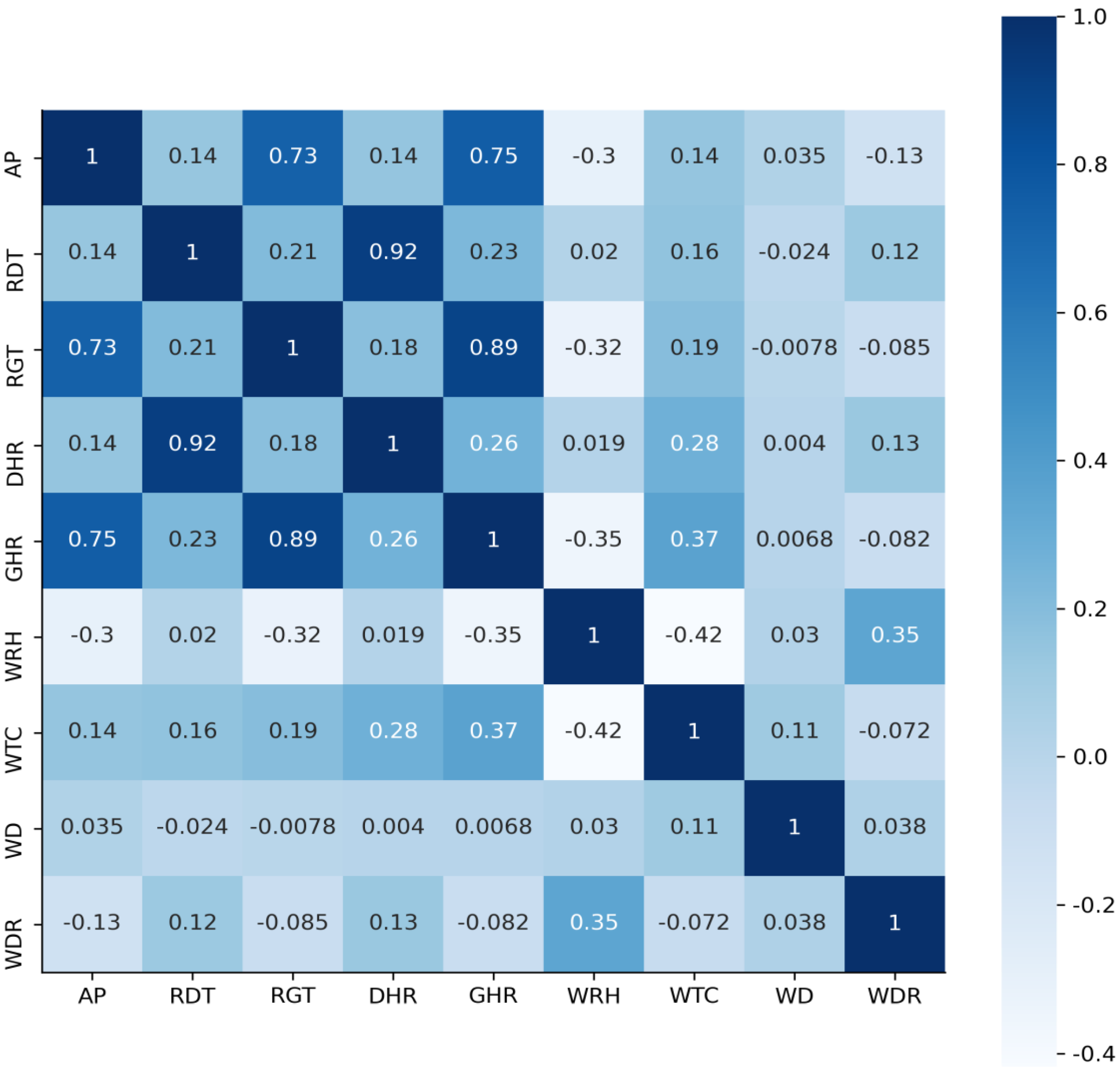
The rest of the study is arranged as follows. Section 2 presents a literature review of the photovoltaic-power-generation-prediction models. Section 3 introduces the sources and the processing of the data. In this section, the pre-processing of relevant features, such as filling in missing values, is conducive to improving the performance of the prediction model. Section 4 describes the four stacking models. 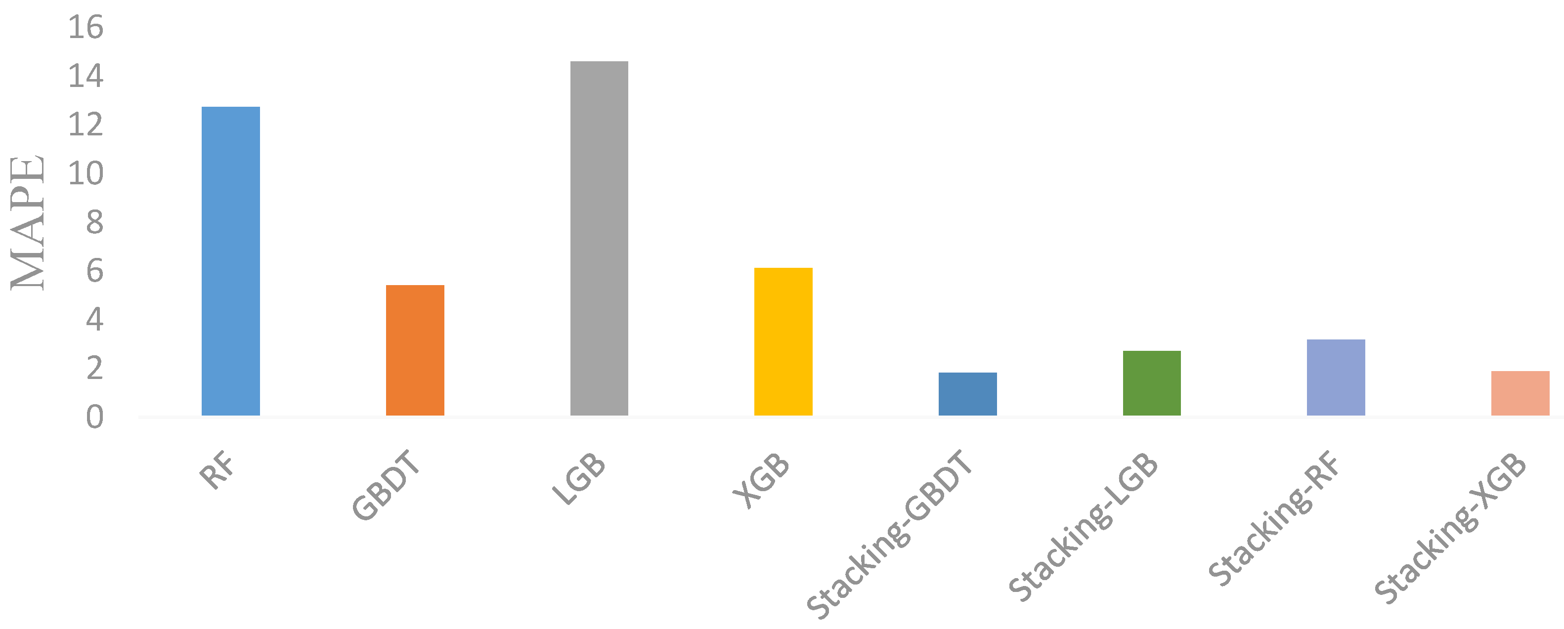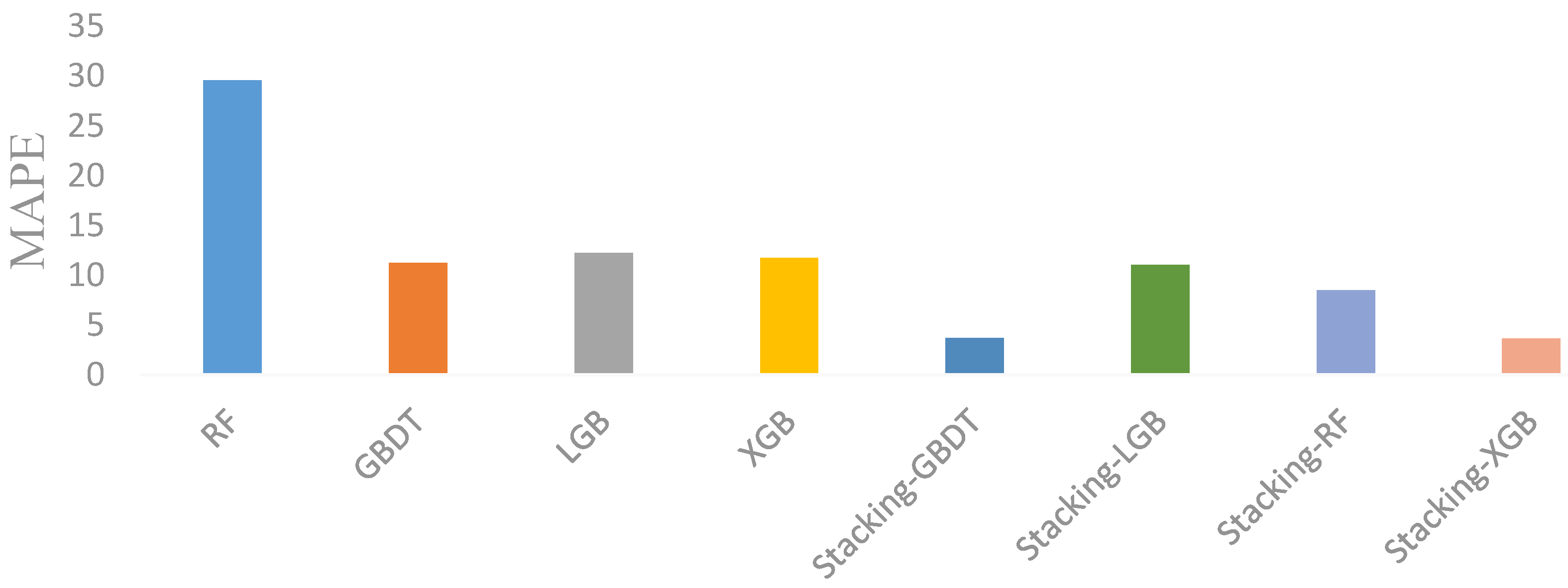Section 5 presents the empirical results of this study, which show that the stacking model has a better prediction accuracy than the single machine-learning model. The Stacking-GBDT model has the highest predictive accuracy among the stacking models that are presented in this study. In Section 6, we draw a conclusion and suggest future directions for research.

2. Related Work

PV-generation prediction is very important in power-grid dispatching and for power-market transactions. The accurate prediction of the PV generation is not only beneficial to power-enterprise decisionmakers for improvement in the operation planning of power systems, but it can also provide valuable guidance for power enterprises in the formulation of power production plans and control power reserves, and in the evaluation of purchase and sales contracts. The research on photovoltaic-power-generation prediction has obtained a significant number of research results. According to the different research methods, the research can be divided into traditional models and machine-learning models.

Among the traditional models, the auto-regression comprehensive moving average is the most widely used. For example, Chu et al. (2015) predicted the photovoltaic power generation of an American power station by constructing an ARMA model [5]. Li et al. (2014) improved the ARMA model and proposed the auto-regressive moving average with exogenous variables, and they tested the model by using Chinese data [6]. Some scholars have also used the spatial auto-regression ARMA model to predict the photovoltaic power generation of Portugal. Compared to the ARMA model, the ARMAX model has higher accuracy [4]. In addition, bottom-up and up-scaling approaches are also used to forecast PV generation. For example, Koster et al. (2019) used a bottom-up approach to predict the PV generation of a power station in Germany [21]. Iea et al. (2020) used an up-scaling approach to forecast the PV generation of power stations in Italy and The Netherlands [22]. Although the traditional method can forecast photovoltaic power, it has a limited ability to deal with the nonlinear relationship between multidimensional data and variables. However, the factors that affect the photovoltaic power generation are multidimensional, and their relationship with the power generation is nonlinear, which leads to the poor prediction performance of traditional statistical methods.

Machine learning is a multidisciplinary specialty that covers probability theory, statistical approximation theory, and complex algorithms. It uses algorithms to extract valuable information and knowledge from existing data [23]. Machine learning is common in many fields of research because of its advantages in processing multidimensional and nonlinear data [23]. Over the years, researchers have adopted classical machine-learning models, such as SVR, SVM, and neural networks, to forecast photovoltaic power generation. Rana et al. (2016) constructed an SVR model to forecast the PV power generation of power stations located in Australia [24]. Gigoni et al. (2018) constructed an SVR model to forecast the PV power generation of power stations located in Italy [25]. Dewangan et al. (2020) constructed an SVR model to forecast the PV power generation of power stations located in Australia [26]. Some scholars also use SVM models to predict the photovoltaic power generation, such as Shi et al. (2012), who constructed an SVM model to forecast the PV power generation of power stations located in China [27]. Liu et al. (2019) constructed an SVM model to forecast the PV power generation of power stations located in Australia [28]. Neural networks are computing systems that are inspired by, but are not identical to, the biological neural networks that make up the brains of animals, and they include ANN, DNN, RNN, and others. Neural networks are nonlinear statistical-data-modeling tools that are used to model the complex relationship between input and output. A number of scholars have used ANN models to predict photovoltaic power generation with different datasets [25,27,29,30,31,32,33,34]. Ramsami and Oree (2015) predicted Britain’s photovoltaic power generation by using an RNN model [35]. Sharadga et al. (2020) constructed an RNN model to forecast the photovoltaic power generation in Mauritius [36]. When RNN cells face long sequences of data, it is easy to encounter gradient discretization, which endows the RNN with only a short-term memory. In other words, when faced with long sequences of data, an RNN can only obtain the information of the relatively recent sequence; however, it does not have the memory function of the earlier sequence, and it thus loses the information. Therefore, researchers have proposed the LSTM method to solve such problems [37]. Many scholars use the LSTM model to forecast photovoltaic power generation [38,39,40]. For example, Dewangan et al. (2020) constructed an LSTM model to forecast photovoltaic power generation in Australia [26]. Li et al. (2020 compared the prediction accuracies of the LSTM model and the RNN model, and the research results show that the LSTM model has a high prediction accuracy [41].

With the development of technology, scholars continue to develop ensemble-learning algorithms, and they have found that ensemble-learning algorithms can improve the prediction accuracies of models [42]. Ensemble learning is a machine-learning method that uses a series of models to learn, and it uses certain rules to integrate the learning results of each model so as to achieve better prediction results than a single model. Ensemble learning is a very popular machine-learning algorithm. It is not a single machine-learning algorithm; instead, it builds multiple models on the data and integrates the modeling results of all of the models. So far, scholars have developed a variety of ensemble-learning algorithms, which can be divided into bagging, boosting, and stacking, according to different integration strategies. (1) The bagging algorithm uses all of the features to train the basic learning-machine model, it samples a large amount of data in parallel at one time, and it outputs the predicted results of each basic learner through a combination strategy. RF is a machine-learning model that is based on bagging ideas. Random forest is an algorithm that integrates multiple trees through the idea of ensemble learning, and its basic units are decision trees [43]. Sun et al. (2016) constructed an RF model to forecast the solar radiation of different photovoltaic power stations in China [44]. (2) The boosting algorithm was first proposed by Kearns (1988) [17]. On the basis of this algorithm, scholars have proposed the gradient boosting decision tree (GBDT), extreme gradient boosting (XGB), and light gradient boosting (LGB) [45]. Hassan et al. (2017) compared the GBDT model to the corresponding MLP, SVR, and DT [8]. They found that the GBDT model is relatively simple, but that it has high reliability and accuracy in photovoltaic power prediction. Pedro et al. (2018) found that the GBDT has a higher accuracy than the KNN model [10]. Kumari and Toshniwal (2021) combined XGB with DNN and proposed the XGB-DNN model [46]. (3) Stacking is an ensemble framework of the layered model that was proposed by Wolpert (1992) [47]. In simple terms, stacking is learning a new learner through the use of the prediction results of several base learners as a new training set after learning several base learners from the initial training data. Stacking models can prevent over-fitting and can improve the accuracy of prediction. Ting and Witten (1999) confirm that the stacking model has a higher accuracy than the basic model [48]. Ke et al. (2021) constructed an XGB model, an LR model, an LGB model, and a stacking model to predict the subjective wellbeing of residents, and they found that the stacking model had a significant advantage in terms of accuracy [49]. Cao et al. (2019) used a stacking model to forecast individual credit. The results show that the stacking model has high prediction accuracy [50].

Although the models that have been developed and that are based on ensemble algorithms have been widely used in photovoltaic power prediction, there are still some limitations in the related research. Most studies use one of the ensemble algorithms to construct a model. In this article, we focus on a stacking model that is based on an ensemble-algorithm model. It consists of multiple base models (XGB, RF, GBDT, and LGB).

3. Data and Preprocessing

3.1. Data

In this study, we used two datasets: one from Australia and the other from China. The data points from the Australian dataset (Dataset A) were taken every five minutes, and the time span was from 1 January 2018 to 10 September 2021. The dataset includes power-generation data and meteorological data (light, temperature, humidity, rainfall, etc.). The variable definitions are shown in

Table 1. Variables and definitions (Dataset A).

Variable	Definition	Unit	Mean
Active Power (AP)	Sampled at 10-s intervals and average power over five min.	kW	2.2877
Weather Temperature Celsius (WTC)	Weather temperature Celsius sampled at 10-s intervals and averaged over 5 min.	°C	26.0944
Weather Relative Humidity (WRH)	Weather relative humidity sampled at 10-s intervals and averaged over 5 min.	%	24.6945
Global Horizontal Radiation (GHR)	Intensity of solar power received by a horizontal plane at the surface of the Earth.	W/m2	574.7895
Diffuse Horizontal Radiation (DHR)	Light that has been scattered by atmospheric particles not in the line of direct radiation from the sun.	W/m2	106.2074
Wind Direction (WD)	Wind direction sampled at 10-s intervals and averaged over 5 min.	°	44.3423
Weather Daily Rainfall (WDR)	Weather daily rainfall sampled at 10-s intervals and averaged over 5 min.	mm	0.3100
Radiation Diffuse Tilted (RDT)	Light that has been scattered by atmospheric particles not in the line of direct radiation from the sun.	W/m2	114.1550
Radiation Global Tilted (RGT)	Intensity of solar power received by the array tilted plane at the surface of the Earth.	W/m2	611.6500

. We chose this dataset as the core dataset of our model because the sampling frequency of the data points is high and it generates a lot of data, which meets the machine-learning-data requirements in this paper. The time series of the sampling (every five minutes) matches the prediction level that we wanted. Photovoltaic power is affected by weather factors that vary from moment to moment. Therefore, the more detailed the time, the higher the accuracy of the prediction, and the more conducive to the adjustment of the power-supply scheme at any time by power enterprises.

The PV power time-series diagram of a particular day is shown in Figure 1. As is shown in the figure, the power that was generated before 6 a.m. and after 8 p.m. is 0; this is because the photovoltaic power generation is mainly determined by the solar illumination intensity. In this paper, datasets between 6 a.m. and 8 p.m. were selected in order to ensure that the power that is generated is greater than 0. Throughout the day, the generating power fluctuates with time, and it reaches its peak at noon.

A cross-sect’'s generality and robustness. There are 17,295 records in this dataset, and each record includes power-generation data, meteorological data (light intensity, temperature, wind direction, etc.), and generator-board-performance data (the heat dissipation performance and the conversion efficiency of the generator board). The variable definitions are shown below (See

Table 2. Variables and definitions (Dataset B).

Variable	Definition	Unit	Mean
Active Power (AP)	Average power of photovoltaic panels over time.	W	3080.3921
Photoelectric Plate Temperature (PPT)	Average temperature of photovoltaic panels over time.	°C	6.7673
Weather Temperature (WT)	Average ambient temperature over time.	°C	0.1890
Light Intensity (LI)	Average light intensity over time.	-	342.5009
Transfer Efficiency (TE)	Historical average conversion efficiency of photovoltaic panels.	-	60.0630
Wind Direction (WD)	Average wind speed over time.	°	223.6044
Wind Speed (WS)	Average wind direction over time.	m/s	2.3855

).

3.2. Preprocessing

For general machine learning, the classification and prediction usually require data entry, data cleaning, feature extraction, feature screening, model training, model evaluation, and other steps. Among them, data cleaning and screening are the preparatory work before model training. Data cleaning is performed mainly in order to process the data that are exported from the information system, to a certain extent, to remove the nonstandard data and some useless and disorderly data, which include data anomalies, and to check missed value processing and abnormal value processing. For missing data, we took the average value of the data at two nearby similarity points and filled it in. For data that suddenly become abnormally large, or suddenly become zero, we filled them in with the average value of the data. In Dataset A, as all of the wind-speed variables were missing, the influence of the wind speed on the predicted results was not considered in the model. A thermal diagram of the correlation coefficients was drawn (Figure 2). As shown in Figure 2, except for rainfall and relative humidity, which were negatively correlated with tilted PV power, other variables showed positive correlations, with the global horizontal radiation and the tilted global radiation having the largest correlation coefficients.

4. Prediction model

4.1. Random Forest

Random forest is an integration model that is based on bagging, and it establishes many decision trees and form forests in a random way [51]. Random forest is a representative ensemble algorithm. All of its base estimators are decision trees. The forest that is composed of classification trees is called the “random forest classifier”, and the forest ensemble by regression trees is called “random forest regression”. The basic steps of training a random forest model can be described as follows: (1) bootstrap sampling is used to form k training subsets (D_k); (2) m features are randomly selected from the original features; (3) we train the training subset (D_k), make the optimal segmentation of m randomly selected features, and obtain k decision tree prediction results; and (4) we determine the final result from the k predictions.

In the bagging process, the algorithm builds multiple models from the same original sample dataset in order to reduce the variance (shown in Figure 3). Random forest is an application of bagging in addition to building trees that are based on different bagging samples from the original training data. Random forest algorithms constrain the features that can be used to build the trees, which forces the trees to be different. To date, random forest models have been widely applied to various research fields [51].

4.2. Extreme Gradient Boosting

Extreme gradient boosting (XGB) is a new method that was proposed by Chen and Guestrin [16]. Different from RF models that use the bagging integration method, XGB is an ensemble tree model that integrates CART tree with the boosting method, which has the advantages of a faster training speed than other common machine-learning methods, since it can efficiently process large amounts of data in a parallel way [42]. The output is the sum of the predicted scores of all the CART trees, which can be expressed as Equation (1):

$$\stackrel{\wedge }{y}={\displaystyle {\sum }_{n=1}^N{f}_m(X)}$$

(1)

where $N$ is the number of trees in the model; $f_m$ is the independent CART of the model; and $\stackrel{\wedge }{y}$ is the predicted value of the model.

The base learner of XGB is a regression tree, and its residual fitting process can be expressed as Equation (2):

$$\{\begin{array}{c}{\stackrel{\wedge }{y_l}}^{(0)}=0\\ {\stackrel{\wedge }{y_l}}^{(1)}={\stackrel{\wedge }{y_l}}^{(0)}+f_1(x_i)\\ {\stackrel{\wedge }{y_l}}^{(2)}={\stackrel{\wedge }{y_l}}^{(1)}+f_2(x_i)\\ {\stackrel{\wedge }{y_l}}^{(t)}={\stackrel{\wedge }{y_l}}^{(t+1)}+f_t(x_i)\end{array}$$

(2)

where ${\stackrel{\wedge }{y_l}}^{(t)}$ is the predicted value of t iterations of the i sample; and ${\stackrel{\wedge }{y_l}}^{(0)}$ is the initial value of the i sample.

According to the iterative process of residuals, the objective optimization function (loss function) of the algorithm can be obtained as shown in Equation (3):

$$f_{obi}^{(t)}={\displaystyle {\sum }_{i=1}^{n}l(y_i},{\stackrel{\wedge }{y_l}}^{(t)})+{\displaystyle {\sum }_{i=1}^t\mathsf{\Omega }(f_i})$$

(3)

XGB performs second-order Taylor expansion for general loss functions in order to extract more information about gradients and to better train gradient descent methods by removing constant terms. The loss function of the t step is shown in Equation (4):

$$\{\begin{array}{c}{g}_i={\partial }_{y_i^{(t-1)}}l(y_i,{\stackrel{\wedge }{y_l}}^{(t)})\\ h_i={\partial }_{{}_{y_i^{(t-1)}}}^{2}l(y_i,{\stackrel{\wedge }{y_l}}^{(t)})\end{array}$$

(4)

where $g_i$ is the first-order partial derivative of the function, and $h_i$ is the second-order partial derivative of the function.

4.3. GBDT and LGB

The gradient boost decision tree (GBDT) is a boosting ensemble-learning algorithm that uses a gradient-lifting algorithm to train the decision-tree model. The model is composed of multiple classification regression trees, and a high-performance learning method is formed by integrating the weak-learner decision tree into the training. The optimal division of the decision tree is found by finding the minimum mean square deviation, and the real value is gradually iterated to optimize the prediction accuracy of the model. Gradient boost decision tree has excellent performance in processing multifeature input classification and regression, and the model training speed is fast, and the accuracy is high.

LGB is a distributed-gradient-lifting framework that is based on a decision-tree algorithm, which is a variant of the gradient boost decision tree. Its basic principle is basically consistent with the GBDT principle. However, through the linear combination of weak regression trees into strong regression trees, and because of the adoption of the histogram and leaf-wise decision-tree optimization algorithm, LGB can reduce the memory occupation of the data calculation, ensure the use of as many data as possible without sacrificing speed, realize parallel computing learning, and support large-scale data processing.

The stacking algorithm is an ensemble learning method. It differs from bagging and boosting in that stacking algorithms can integrate different types of models, while bagging and boosting are generally the same type of model. The great advantage of stacking algorithms is that the benefits of combining different models can be analyzed from a variety of perspectives, which results in the better predictive performance of the model. On the basis of the stacking algorithm, we built four stack models. The four stack models are shown below (See

Table 3. The four proposed models.

Model Name	Base Models	Stacking Layers
Stacking-GBDT	XGB, LGB, and RF	GBDT
Stacking-LGB	XGB, GBDT, and RF	LGB
Stacking-RF	XGB, LGB, and GBDT	RF
Stacking-XGB	GBDT, LGB, and RF	XGB

).

For the Stacking-GBDT model, XGB, LGB, and RF are used as the base models and the gradient boosting decision tree (GBDT) is used as the stacking-layers-2 model, as is shown in Figure 4. For the Stacking-LGB model, GBDT, LGB, and RF are used as the base models and XGB as the stacking-layers-2 model. For the Stacking-LGB model, GBDT, XGB, and RF are used as the base models, and LGB as the stacking-layers-2 model. For the Stacking-RF model, GBDT, XGB, and LGB are used as the base models, and RF as the stacking-layers-2 model.

4.4. Model-Performance Evaluation

To determine which model is highly predictive, the mean absolute error (MAE), the root mean absolute error (RMAE), the mean squared error (MSE), the root mean squared error (RMSE), and the mean absolute percent error (MAPE), which are commonly used in the field of statistics to measure the prediction accuracy of models, were selected as the evaluation criteria for the models’ performances in this study.

5. Experiments and Results

5.1. Test Environment

To determine which model is highly predictive, the experiment was carried out on a computer. All of the model results were implemented by using the machine-learning library that is provided by Python.

5.2. Dataset-A Results

We chose 70% of the data as the training dataset, and the rest as the test dataset. Figure 5 shows the optimal model (Stacking-GBDT) iteration process. As can be seen from the figure, the model loss decreases with the increase in the iteration times, and then the stable value is preserved. Moreover, the decreased speed of the loss of the test set is lower than that of the training set. When the loss function reaches a stable value, the test-set loss-function value is always higher than the train-set loss-function value.

Table 4. The results for different prediction methods (Dataset A).

Model Classification	Model	MAE	RMAE	MSE	RMSE	MAPE
Traditional model	LR	0.6687	0.8177	1.1308	1.0634	14.2064
Single machine-learning model	RF	0.4787	0.6919	0.6982	0.8356	12.7396
	GBDT	0.2747	0.5241	0.2892	0.5378	5.4112
	LGB	0.3311	0.5754	0.2605	0.5104	14.6022
	XGB	0.3084	0.5553	0.3637	0.6031	6.1291
Stacking model	Stacking-GBDT	0.1269	0.3562	0.0990	0.3147	1.8175
	Stacking-LGB	0.1509	0.3885	0.1626	0.4032	2.7157
	Stacking-RF	0.1463	0.3825	0.1103	0.3321	3.1861
	Stacking-XGB	0.1276	0.3572	0.0989	0.3145	1.8765

shows that the LR model has the lowest prediction accuracy. The prediction performance of the single machine-learning model is better than that of the LR model. By comparing the prediction accuracy of RF, GBDT, LGB, and XGB, it is shown that the MAEs of the four models increase gradually in the following order: GBDT (0.2747) < XGB (0.3084) < LGB (0.3311) < RF (0.4787). It is shown that the forecast error of the stacking model is generally lower than that of the single ensemble-learning model. We further compared the prediction accuracies of different stacking models, and we found that the MAEs of the stacking models increase gradually in the following order: Stacking-GBDT (0.1269) < Stacking-XGB (0.1276) < Stacking-RF (0.1463) < Stacking-LGB (0.1509). However, for the MSEs, the order is: Stacking-XGB (0.0989) < Stacking-GBDT (0.0990) < Stacking-RF (0.1103) < Stacking-LGB (0.1626).

Table 5. The prediction errors for a small testing set (Dataset A).

Actual Values	Predicted Values	Absolute Values of Prediction Errors
2.2000	2.0785	0.1215
3.1071	3.0989	0.0082
0.2888	0.3189	0.0301
1.3631	1.4277	0.0646
4.0310	4.0548	0.0237
0.0302	0.0250	0.0052
4.5923	4.6104	0.0181
3.3361	3.2962	0.0399
1.4187	1.4191	0.0004
0.2576	0.2319	0.0257

shows the actual values, the predicted values, and the prediction errors of some of the datasets of the Stacking-GBDT model. The results show that the prediction error is small, which indicates that the model has good prediction performance.

Figure 6 also shows that the forecast performance of the Stacking-GBDT model is better than the other stacking models. The results show that Stacking-GBDT is a promising photovoltaic-power-generation-capability-prediction method. Overall, the Stacking-GBDT model has the best predictive performance.

5.3. Dataset-B Results

Unlike Dataset A, Dataset B contains cross-sectional data. Dataset B, from a photovoltaic power station in China, was used to test the model’s generality and robustness. We chose 70% of the data as the training dataset, and the rest as the test dataset. The prediction errors of the different models are shown below.

Table 6. The results for different methods (Dataset B).

Model Classification	Model	MAE	RMAE	MSE	RMSE	MAPE
Traditional model	LR	942.9077	30.7068	6953.7619	83.3892	66.8734
Single machine-learning model	RF	431.2076	20.7655	2367.1626	48.6535	29.5431
	GBDT	178.6581	13.3663	2143.8647	46.3019	11.2456
	LGB	245.1807	15.6582	3724.2502	61.0266	12.2411
	XGB	208.3785	14.4353	2492.8748	49.9287	11.7427
Stacking model	Stacking-GBDT	106.0726	10.2992	2283.1803	47.7826	3.6621
	Stacking-LGB	125.5729	11.2059	2332.5951	48.2969	11.0491
	Stacking-RF	161.7984	12.7200	2313.3848	48.0977	8.4549
	Stacking-XGB	111.3737	10.5534	2506.2799	50.0628	3.6494

shows that the LR model has the lowest prediction accuracy. The prediction performance of the single machine-learning model is better than that of the LR model. We further compared the prediction accuracies of different stacking models, and we found that the MAEs of the stacking models increase gradually in the following order: Stacking-GBDT (106.0726) < Stacking-XGB (111.3737) < Stacking-RF (125.5729) < Stacking-LGB (161.7984). The MSEs of the stacking models increase gradually in the following order: Stacking-GBDT (2283.1803) < Stacking-RF (2313.3848) < Stacking-LGB (2332.5951) < Stacking-XGB (50.0628).

Table 7. The prediction errors for a small testing set (Dataset B).

Actual Values	Predicted Values	Absolute Values of Prediction Errors
3416.6700	3435.3855	18.7155
4360.2200	4371.3931	11.1731
3334.5600	3340.9911	6.4311
1761.7900	1758.2486	3.5413
2105.1600	2093.7150	11.4449
1093.7500	1085.9514	7.7985
1811.4700	1813.4159	1.9459
907.7200	901.6197	6.1002
4347.2500	4372.0754	24.8254
5023.2700	5031.0504	7.7804

shows the actual values, the predicted values, and the prediction errors of some datasets of the Stacking-GBDT model. The results show that the prediction error is small, which indicates that the model has good prediction performance.

Figure 7 also shows that the Stacking-GBDT and Stacking-XGB models have better prediction accuracies than the Stacking-RF and Stacking-LGB models for different prediction horizons. To summarize, the Stacking-GBDT model has the best predictive performance.

6. Discussion and Conclusions

The most effective way to achieve peak carbon and carbon neutrality is to reduce carbon emissions by using renewable energy. Solar energy is a renewable energy that can reduce carbon emissions and achieve carbon neutrality. However, the unique random intermittency and the fluctuation of solar energy present many challenges to the safety of power grids with the increasing demand for photovoltaic installed capacities. The accurate forecasting of PV power generation is helpful for grid-planning improvement, scheduling optimization, and management development. Machine-learning models have high predictive accuracies, and they are widely used in various fields, including in photovoltaic power generation.

Although machine learning has been used by scholars to predict photovoltaic power generation, most studies use the single machine-learning model. In recent years, scholars have developed ensemble-learning algorithms that can significantly improve the performance of the model. The stacking model is one of the most popular ensemble-learning algorithms that is currently being applied to different prediction models.

In this work, four ensemble-learning algorithms (XGB, RF, LGB, and GBDT) were selected to build four stacking models to predict photovoltaic power generation. The four stacking models are: Stacking-GBDT, Stacking-XGB, Stacking-RF, and Stacking-LGB. We used two datasets to test the predictive performances of the different models. Data points from the Australian dataset (Dataset A) were taken every five minutes, and the time span was from 1 January 2018 to 10 September 2021. The results show that the stacking model has high prediction performance. Our results lead us to the following conclusions:

• The prediction performance of the four stacked models is better than that of the single machine-learning model. First, by using Australian panel data, the prediction performance of the stacked model is better than that of the single machine-learning model. Second, by using Chinese cross-sectional data, the robustness of the conclusion is verified again;
• The Stacking-GBDT model has a higher prediction accuracy than the Stacking-XGB model, the Stacking-RF model, and the Stacking-LGB model. By comparing the prediction accuracies of the above models by using the Australian dataset, it was found that the Stacking-GBDT model had the highest prediction accuracy, which was also verified by the Chinese dataset;
• Machine-learning models have better prediction accuracies than traditional LR models, on the whole. In the research, we compared the prediction accuracy of a single machine-learning model with that of a traditional linear regression model. We found that the prediction accuracy of the single machine-learning model is higher than the traditional linear regression model. This conclusion is consistent with previous studies.

Although this study contributes to the literature on photovoltaic-power-generation prediction, it has several limitations. In this work, LGB, XGB, and random forest were only used as the base models of the stacking model to predict the photovoltaic power generation. In the future, more machine-learning models could be used as the first layer of the stacking model in order to conduct a more detailed division and analysis of the model architecture. Data from Australia and China were used in this study. Data from other countries can be considered in future studies to overcome the limitations in the two countries, and to expand the universal applicability of the model.

References

1. In 2050, Photovoltaics Will Become the Largest Power Source in China. Available online: https://new.qq.com/omn/20211025/20211025A0AWI700.html (accessed on 4 April 2022).
2. Dimd, B.D.; Call, S.V.U.; Midtgard, O.M. A Review of Machine Learning-Based photovoltaic Output Power Forecasting: Nordic Context. IEEE Access 2022, 10, 26404–26425. [Google Scholar] [CrossRef]
3. Bacher, P.; Madsen, H.; Nielsen, H.A. Online short-term solar power forecasting. Sol. Energy 2009, 83, 1772–1783. [Google Scholar] [CrossRef] [Green Version]
4. Bessa, R.J.; Trindade, A.; Silva, C.; Miranda, V. Solar power forecasting in smart grids using distributed information. Int. J. Electr. Power Energy Syst. 2015, 72, 16–23. [Google Scholar] [CrossRef] [Green Version]
5. Chu, Y.; Urquhart, B.; Gohari, S.; Pedro, H.T.; Kleissl, J.; Coimbra, C.F. Short-term reforecasting of power output from a 48 MWe solar PV plant. Sol. Energy 2015, 112, 68–77. [Google Scholar] [CrossRef]
6. Li, Y.; Yan, S.; Shu, L. An ARMAX model for forecasting the power output of a grid connected photovoltaic system. Renew. Energy 2014, 66, 78–89. [Google Scholar] [CrossRef]
7. Lou, S.; Li, D.; Lam, J.C.; Chan, W.W.H. Prediction of diffuse solar irradiance using machine learning and multivariable regression. Appl. Energy 2016, 181, 367–374. [Google Scholar] [CrossRef]
8. Hassan, M.A.; Khalil, A.; Kaseb, S.; Kassem, M.A. Exploring the potential of tree-based ensemble methods in solar radiation modeling. Appl. Energy 2017, 203, 897–916. [Google Scholar] [CrossRef]
9. Fouilloy, A.; Voyant, C.; Notton, G.; Motte, F.; Paoli, C.; Nivet, M.-L.; Guillot, E.; Duchaud, J.-L. Solar irradiation prediction with machine learning: Forecasting models selection method depending on weather variability. Energy 2018, 165, 620–629. [Google Scholar] [CrossRef]
10. Pedro, H.; Coimbra, C.; David, M.; Lauret, P. Assessment of machine learning techniques for deterministic and probabilistic intra-hour solar forecasts. Renew. Energy 2018, 123, 191–203. [Google Scholar] [CrossRef]
11. Yagli, G.M.; Yang, D.Z.; Srinivasan, D. Automatic hourly solar forecasting using machine learning models. Renew. Sustain. Energy Rev. 2019, 105, 487–498. [Google Scholar] [CrossRef]
12. Babar, B.; Luppino, L.T.; Bostrm, T.; Anfinsen, S.N. Random forest regression for improved mapping of solar irradiance at high latitudes. Sol. Energy 2020, 198, 81–92. [Google Scholar] [CrossRef]
13. Narvaez, G.; Giraldo, L.F.; Bressan, M.; Pantoja, A. Machine Learning for Site-adaptation and Solar Radiation Forecasting. Renew. Energy 2021, 167, 333–342. [Google Scholar] [CrossRef]
14. Lee, J.; Wang, W.; Harrou, F.; Sun, Y. Reliable solar irradiance prediction using ensemble learning-based models: A comparative study. Energy Convers. Manag. 2020, 208, 112582. [Google Scholar] [CrossRef] [Green Version]
15. Gupta, P.; Singh, R. PV power forecasting based on data driven models: A review. Int. J. Sustain. Eng. 2021, 14, 1733–1755. [Google Scholar] [CrossRef]
16. Chen, T.Q.; Guestrin, C. XGBoost: A scalable tree boosting system. In Proceedings of the 22nd ACM SIGKDD International Conference on Knowledge Discovery and Data Mining, San Francisco, CA, USA, 13–17 August 2016; pp. 785–794. [Google Scholar]
17. Kearns, M. Thoughts on Hypothesis Boosting. 1988. Available online: https://www.studocu.com/en-us/document/university-of-pennsylvania/the-algorithmic-foundations-of-data-privacy/thoughts-on-hypothesis-boosting-old-class-project-for-notes/725678 (accessed on 18 March 2022).
18. Breiman, L. Bagging Predictors. Mach. Learn. 1996, 46, 50. [Google Scholar] [CrossRef] [Green Version]
19. Guo, X.; Gao, Y.; Zheng, D.; Ning, Y.; Zhao, Q.N. Study on short-term photovoltaic power prediction model based on the Stacking ensemble learning. Energy Rep. 2020, 6, 1424–1431. [Google Scholar] [CrossRef]
20. Eom, H.; Son, Y.; Choi, S. Feature-Selective Ensemble Learning-Based Long-Term Regional PV Generation Forecasting. IEEE Access 2020, 8, 54620. [Google Scholar] [CrossRef]
21. Koster, D.; Minette, F.; Braun, C.; O’Nagy, O. Short-term and regionalized photovoltaic power forecasting, enhanced by reference systems, on the example of Luxembourg. Renew. Energy 2019, 132, 55–470. [Google Scholar] [CrossRef]
22. Iea, D.; Pierro, M.; Cornaro, C.; Moser, D. Regional Solar Power Forecasting. Available online: https://www.researchgate.net/publication/345163894_Regional_solar_power_forecasting (accessed on 4 April 2022).
23. Molina, M.; Garip, F. Machine Learning for Sociology. Annu. Rev. Sociol. 2019, 45, 27–45. [Google Scholar] [CrossRef] [Green Version]
24. Rana, M.; Koprinska, I.; Agelidis, V.G. Univariate and multivariate methods for very short-term solar photovoltaic power forecasting. Energy Convers. Manag. 2016, 121, 380–390. [Google Scholar] [CrossRef]
25. Gigoni, L.; Betti, A.; Crisostomi, E.; Franco, A.; Tucci, M.; Bizzarri, F.; Mucci, D. Day-Ahead Hourly Forecasting of Power Generation from photovoltaic Plants. IEEE Trans. Sustain. Energy 2017, 9, 831–842. [Google Scholar] [CrossRef] [Green Version]
26. Dewangan, C.L.; Singh, S.N.; Chakrabarti, S. Combining forecasts of day-ahead solar power. Energy 2020, 202, 117743. [Google Scholar] [CrossRef]
27. Shi, J.; Lee, W.J.; Liu, Y.Q.; Yang, Y.Y.; Wang, P. Forecasting Power Output of photovoltaic Systems Based on Weather Classification and Support Vector Machines. IEEE Trans. Ind. Appl. 2012, 48, 1064–1069. [Google Scholar] [CrossRef]
28. Liu, L.; Zhan, M.; Bai, Y. A recursive ensemble model for forecasting the power output of photovoltaic systems. Sol. Energy 2019, 189, 291–298. [Google Scholar] [CrossRef]
29. Pedro, H.; Coimbra, C. Assessment of forecasting techniques for solar power production with no exogenous inputs. Sol. Energy 2012, 86, 2017–2028. [Google Scholar] [CrossRef]
30. Zhu, H.; Li, X.; Sun, Q.; Nie, L.; Yao, J.; Zhao, J. A Power Prediction Method for photovoltaic Power Plant Based on Wavelet Decomposition and Artificial Neural Networks. Energies 2016, 9, 11. [Google Scholar] [CrossRef] [Green Version]
31. Rosiek, S.; Alonso-Montesinos, J.; Batlles, F.J. Online 3-h forecasting of the power output from a BIPV system using satellite observations and ANN. Int. J. Electr. Power Energy Syst. 2018, 99, 261–272. [Google Scholar] [CrossRef]
32. Bae, K.Y.; Han, S.J.; Bang, C.J.; Sung, D.K. Effect of Prediction Error of Machine Learning Schemes on photovoltaic Power Trading Based on Energy Storage Systems. Energies 2019, 12, 1249. [Google Scholar] [CrossRef] [Green Version]
33. Yang, H.T.; Huang, C.M.; Huang, Y.C.; Pai, Y.S. A Weather-Based Hybrid Method for 1-Day Ahead Hourly Forecasting of PV Power Output. IEEE Trans. Sustain. Energy 2014, 5, 917–926. [Google Scholar] [CrossRef]
34. Eseye, A.T.; Zhang, J.; Zheng, D. Short-term photovoltaic solar power forecasting using a hybrid Wavelet-PSO-SVM model based on SCADA and Meteorological information. Renew. Energy 2017, 118, 357–367. [Google Scholar] [CrossRef]
35. Ramsami, P.; Oree, V. A hybrid method for forecasting the energy output of photovoltaic systems. Energy Convers. Manag. 2015, 95, 406–413. [Google Scholar] [CrossRef]
36. Sharadga, H.; Hajimirza, S.; Balog, R.S. Time series forecasting of solar power generation for large-scale photovoltaic plants. Renew. Energy 2020, 150, 797–807. [Google Scholar] [CrossRef]
37. Hochreiter, S.; Schmidhuber, J. Long Short-Term Memory. Neural Comput. 1997, 9, 1735–1780. [Google Scholar] [CrossRef] [PubMed]
38. Zang, H.; Liu, L.; Sun, L.; Cheng, L.; Wei, Z.; Sun, G. Short-term global horizontal irradiance forecasting based on a hybrid CNN-LSTM model with spatiotemporal correlations. Renew. Energy 2020, 160, 26–41. [Google Scholar] [CrossRef]
39. Gao, B.; Huang, X.; Shi, J.; Tai, Y.; Zhang, J. Hourly forecasting of solar irradiance based on CEEMDAN and multi-strategy CNN-LSTM neural networks. Renew. Energy 2020, 162, 1665–1683. [Google Scholar] [CrossRef]
40. Zheng, J.; Zhang, H.; Dai, Y.; Wang, B.; Zheng, T.; Liao, Q.; Song, X. Time series prediction for output of multi-region solar power plants. Appl. Energy 2020, 257, 114001. [Google Scholar] [CrossRef]
41. Li, P.; Zhou, K.; Lu, X.; Yang, S.L. A hybrid deep learning model for short-term PV power forecasting. Appl. Energy 2020, 259, 114216. [Google Scholar] [CrossRef]
42. Dietterich, T.G. Ensemble Methods in Machine Learning; Springer: Berlin/Heidelberg, Germany, 2000; pp. 1–15. [Google Scholar]
43. Yu, Z.; Haghighat, F.; Fung, B.C.M.; Yoshino, H. A decision tree method for building energy demand modeling. Energy Build. 2010, 42, 1637–1646. [Google Scholar] [CrossRef] [Green Version]
44. Sun, H.; Gui, D.; Yan, B.; Liu, Y.; Liao, W.; Zhu, Y.; Lu, C.; Zhao, N. Assessing the potential of random forest method for estimating solar radiation using air pollution index. Energy Convers. Manag. 2016, 119, 121–129. [Google Scholar] [CrossRef] [Green Version]
45. Ke, G.; Meng, Q.; Finley, T.; Wang, T.; Chen, W.; Ma, W.; Ye, Q.; Liu, T.-Y. LightGBM: A highly efficient gradient boosting decision tree. In Proceedings of the 31st Conference on Neural Information Processing Systems (NIPS 2017), Long Beach, CA, USA, 4–9 December 2017. [Google Scholar]
46. Kumari, P.; Toshniwal, D. Extreme gradient boosting and deep neural network based ensemble learning approach to forecast hourly solar irradiance. J. Clean. Prod. 2021, 279, 123285. [Google Scholar] [CrossRef]
47. Wolpert, D.H. Stacked generalization. Neural Netw. 1992, 5, 241–259. [Google Scholar] [CrossRef]
48. Ting, K.M.; Witten, I. Issues in Stacked Generalization. J. Artif. Intell. Res. 1999, 10, 271–289. [Google Scholar] [CrossRef] [Green Version]
49. Ke, N.; Shi, G.; Zhou, Y. Stacking Model for Optimizing Subjective Well-Being Predictions Based on the CGSS Database. Sustainability 2021, 13, 11833. [Google Scholar] [CrossRef]
50. Cao, Z.; Yu, D.; Shi, J.; Zong, S. The Two-layer Classifier Model and its Application to Personal Credit Assessment. Control. Eng. China 2019, 26, 2231–2234. (In Chinese) [Google Scholar]
51. Reiman, L. Random forests. Mach. Learn. 2001, 45, 5–32. [Google Scholar] [CrossRef] [Green Version]
Figure 1. PV output on 1 January 2018.
Sustainability 14 05669 g001
Figure 2. Correlation relationship between PV power and feature variables.
Sustainability 14 05669 g002
Figure 3. RF algorithm flow chart.
Sustainability 14 05669 g003
Figure 4. Example of stacking model (Stacking-GBDT).
Sustainability 14 05669 g004
Figure 5. Loss-function value of train and test (Dataset A).
Sustainability 14 05669 g005
Figure 6. MAPEs of different models (Dataset A).
Sustainability 14 05669 g006
Figure 7. MAPEs of different models (Dataset B).
Sustainability 14 05669 g007