Fuzzy Demand Vehicle Routing Problem with Soft Time Windows

Abstract

Considering the vehicle routing problem with fuzzy demand and fuzzy time windows, a vehicle routing optimization method is proposed considering both soft time windows and uncertain customer demand. First, a fuzzy chance-constrained programming model is established based on credibility theory, minimizing the total logistics cost. At the same time, a random simulation algorithm is designed to calculate the penalty cost of delivery failures caused by demand that cannot be satisfied. In order to overcome the shortcomings of GA, which easily falls into the local optimum in the process of searching, and the slow convergence speed of SA when the population is too large, a hybrid simulated annealing–genetic algorithm is adopted to improve the solution quality and efficiency. Finally, the Solomon standard example is used to verify the effectiveness of the algorithm, and the influence of decision-makers’ subjective cost preference is analyzed.

1. Introduction

The vehicle routing problem with fuzzy demand (VRPFD) is an important research issue regarding vehicle routing with uncertain demand that has been extensively studied in the field of logistics and supply chain management [1]. Almost all customers have demands for pickup and/or delivery of goods within time windows in real logistics distribution processes that cannot be known in advance. Therefore, their demands are set within a fuzzy range. Meanwhile, demands that do not meet the time window and that can lead to delivery failure are addressed by imposing a penalty cost in the model. For example, Hoogeboom et al. [2] proposed an adaptive variable neighborhood search algorithm and an exact polynomial–time algorithm for recalculating path durations based on forward and backward start time intervals. Kuo et al. [3] established a dynamic vehicle routing model with uncertain service time using fuzzy theory, and proposed an improved fuzzy ant colony system (ACS) algorithm to solve the model. The authors employed a cluster insertion algorithm embedded into the ACS, improving the algorithm’s performance.

Based on fuzzy reliability theory, Nadizadeh et al. [4] designed a four-stage heuristic algorithm (HHA) to solve the dynamic capacitated location-routing problem with fuzzy demands (DCLRP-FD). Li et al. [5] proposed a new two-stage tabu search algorithm based on the idea of pre-optimization and then rescheduling to solve the vehicle routing problem with fuzzy demand. Zhang and Fan [6] studied the multi-trip vehicle routing problem with fuzzy demand and time window preferences, considering vehicle travel restrictions and customers’ time window preferences. Lei et al. [7] designed a capacitated vehicle routing problem with stochastic demands (CVRPSD) and time windows and employed an adaptive large neighborhood search (ALNS) heuristic to solve it. They obtained good performance based on testing the modified Solomon instances. Unlike the above studies, a fuzzy chance-constrained programming model is applied to solve the problem of fuzzy requirements in this paper.

Aiming to solve the vehicle routing problem with time windows (VRPTW), Ferreira et al. [8] designed a new variable neighborhood search algorithm that only searches feasible solutions based on a hybrid variable neighborhood tabu search (HVNTS). Qi et al. [9] designed a routing improvement method considering the spatiotemporal proximity of customers, and used the genetic algorithm to conduct spatiotemporal clustering of customers to solve the vehicle routing problem with time windows. Most of the above studies focused on the problem from a single perspective, with less consideration of the impact of soft time windows on delivery cost under the condition of uncertain demand and the setting of penalty factors when the decision-maker’s risk preference leads to delivery failure.

The genetic algorithm has been widely used in logistics. Amiri-Aref et al. [10] established a new mixed-integer nonlinear programming (MINLP) method for a multi-period rectilinear distance center location-dependent relocation problem and used LINGO software to solve small-scale instances, applying two meta-heuristics, the genetic algorithm (GA) and competitive algorithm (ICA), for large-scale instances. These algorithms were also applied in two other papers. As the nonlinear constraints make the algorithm spend too much time on searching, Alizadeh et al. [11] converted them to linear constraints to solve the capacitated location–allocation problem with stochastic demands. They also applied the same software and the two meta-heuristics. The experimental results show that the three methods can achieve high efficiency under the constraints of linearization. Based on the above two studies, Shiripour et al. [12] designed a location–allocation–routing problem for the distribution of injured persons in a disaster response scenario, employing the GA and a discrete ICA algorithm to solve this problem. This case, in Iran, shows that the model is feasible and has high performance. Although the genetic algorithm was successfully applied in the above three papers, there is still room for further improvement due to its inherent disadvantages, such as sensitivity to the initial solution, slow search speed, and weakness in local search.

Multi-stage heuristic algorithms are also a hot research topic. Shen et al. [13] established a low-carbon multi-depot open vehicle routing problem with time windows (MDOVRPTW) model to reduce the cost of third-party logistics. A two-phase algorithm for soft time windows, using particle swarm optimization (PSO) first and tabu search (TS) second, was designed to solve the model. In a similar way, Shi et al. [14] proposed a two-stage heuristic algorithm to deal with the multi-depot vehicle routing problem (MDVRP) for urban households and solid waste collection. Two novel heuristics, sector combination optimization (SCO) for the initial solution and the merge-head and drop-tail (MHDT) strategy for intensification, were utilized to address this problem. Moreover, Wang and Zhou [15] proposed a three-stage heuristic for the vehicle routing problem with time windows and stochastic travel times (VRPTWSTT). They called the stages problem transformation, solution construction, and solution improvement. Yang and Sun [16] proposed a four-stage heuristic algorithm called SIGALNS to solve the electric vehicle routing problem. The sweep heuristic, the greedy heuristic, the adaptive large neighborhood search heuristic, and the intensified method were employed in the four stages. These multi-stage heuristic algorithms have achieved high-quality solutions.

Although the “serial” algorithms have the characteristics of simple structure and easy programming implementation, even if the optimal solution can be obtained by using each one individually, the global optimum may not be ultimately obtained. Once an error occurs in the previous stage, it can lead to propagation and even amplification in the subsequent stage. Shiripour et al. [17] constructed a capacitated location–multi-allocation–routing model to minimize total transportation time. Two heuristics, the standard genetic algorithm (GA) and a combined genetic algorithm and local search (GALS), were utilized for large-scale instances. The experimental results show that high performance can be achieved by using the local search algorithm in GA many times. Subsequently, the authors [18] formulated a mixed-integer linear programming model considering some random factors that influence the travel time between two nodes for the capacitated location–multi-allocation–routing problem. They designed a hybrid GALS and an evolutionary simulated annealing algorithm (ESA) to solve the problem. It easily converged prematurely and had poor local optimization ability, which is a disadvantage of the genetic algorithm. However, the simulated annealing algorithm makes up for the defects; it can effectively avoid falling into the local optimal solution and find the global optimal solution of the objective function by using the Metropolis criterion to optimize the process. Because of its dependence on the initial temperature and other parameters, global convergence required a higher temperature in the removal process, and the evolution rate was slow.

In this paper, the hybrid SA–GA algorithm was designed by combining the genetic algorithm with a simulated annealing algorithm. The simulated annealing algorithm controls the convergence of the algorithm and avoids falling into the local optimal solution. The two algorithms were combined to form a parallel genetic–simulated annealing algorithm, in which only one solution is reserved for each unit of time in the operation, to avoid the interference of useless information and historical data in the search process. The combination of simulated annealing and genetic algorithms can improve the evolutionary ability, optimization performance, and search ability.

In view of uncertain customer demand in the distribution process of e-commerce platforms, this paper proposes a method of vehicle routing optimization with fuzzy demand considering soft time windows and insufficient demand constraints. The fuzzy demand vehicle routing problem with soft time windows (FDVRPSTW) is studied based on the existing VRPFD literature. A model with minimum total cost is established based on the credibility measure theory, adding soft time windows and imposing an additional penalty on the total cost to deal with delivery failures when the demand cannot be satisfied. At the same time, the improved hybrid genetic algorithm is designed to solve the model. Finally, the influence of the decision-maker’s subjective preference on the total cost is analyzed, and the effectiveness of the model is verified by many instances.

The rest of this paper is organized as follows. In Section 2, we describe in detail the problem to be solved. In Section 3, we construct a fuzzy chance-constrained programming model. The implementation of the hybrid heuristic algorithm for solving the model is described in detail in Section 4. The computational results are reported in Section 5. Finally, Section 6 contains a summary and future works.

2. Problem Description

For the problem studied in this paper, only customer demands are fuzzy, and other relevant VRP parameters are known and determined. The soft time windows indicate that the customers have the expected service time window and the maximum tolerance range. When the customers are served within their expected time window, the maximum customer satisfaction is 100%. Customer satisfaction decreases gradually with the increased time beyond the ideal time window. However, service is not allowed outside the maximum time window customers can endure. When the customer demand for the current delivery cannot be satisfied, an additional penalty cost is imposed on the total cost, because the delivery vehicles need to return to the distribution center due to the failure. Finally, on the premise of meeting the demands of vehicle capacity and service time, our goal is to find an optimal distribution plan to minimize both logistics and time cost.

In Figure 1, there is only one distribution center (DC) in the distribution network. Each truck can serve multiple customers, and each customer can only be served at most once. Figure 1a shows a distribution route by which all customer requirements can be met, and Figure 1b shows an example of a distribution failure caused by a delivery vehicle without enough goods at node 5; in this situation, the vehicle needs to return to the distribution center for replenishment.

3. Constructing a Fuzzy Chance-Constrained Programming Model

Suppose consumers want to buy a product that has hit the market early. Based on past shopping experience, the product will be sold at a discount in the future. At this time, consumers are faced with two choices. If they purchase the product at the current original price, they may regret the expensive purchase. If they buy the product at a discount in the future, they may face uncertain factors such as the product being out of stock or code, which may lead to regret over missing the purchase opportunity. This kind of anticipation by the consumer over future risk before making a decision is called anticipated regret. This paper uses $p_d$ and $p_n$ to denote the original selling price and the discounted price of the product per unit, respectively, and $p_d=\delta \cdot p_n$ ($\delta$ is the discount level per product unit).

Sign Convention

In the problems studied in this paper, only customer demands are fuzzy, and other relevant VRP parameters are known and determined. There is only one distribution center (DC) in the distribution network. Each truck can serve multiple customers, and each customer can only be served at most once. At the same time, the soft time windows indicate that the customer has an expected service window and the maximum tolerance range. When the customers are served within the expected time window, the maximum customer satisfaction is 100%. Customer satisfaction decreases gradually with increased time beyond the ideal time window. However, service is not allowed outside the maximum time window customers can endure. When the customer demand for the current delivery cannot be satisfied, an additional penalty cost is imposed on the total cost, because the delivery vehicle needs to return to the distribution center due to the failure. Finally, on the premise of meeting the demands of vehicle capacity and service time, our goal is to find an optimal distribution plan to minimize both the logistics and time cost.

Let $\mathrm{G}=\left(V,E\right)$ denote the distribution network, where $V=\left\{0, 1, 2, \dots , n\right\}$ is the set of distribution center (0) and customers (1–n) and $\mathrm{E}=\left\{\left(i,j\right)|i,j\in V\right\}$ is the set of arcs between two nodes. $c_i$ and $t_{ij}$ denote the travel cost and travel time, respectively, between nodes $i$ and $j$. Available distribution vehicles are denoted by $\mathrm{K}=\left\{1, 2, \dots ,m\right\}$, and all vehicles have the same maximum load capacity $\mathrm{Q}$ and fixed cost $c_0$. Each customer has a time window $\left[E{T}_j^{\prime },E{T}_j,E{L}_j,E{L}_j^{\prime }\right]$, where $\left[E{T}_j,E{L}_j\right]$ denotes the expected service time interval and $\left[E{T}_j^{\prime },E{L}_j^{\prime }\right]$ denotes the maximum tolerance time window, and the four parameters are subject to $E{T}_j^{\prime }\le E{T}_j\le E{L}_j\le E{L}_j^{\prime }$.

In this paper, the fuzzy demands are described by triangular fuzzy numbers $\overline{d}=\left(d_1,d_2,d_3\right)$, where $d_1,d_3$ represents the left and the right boundaries, respectively, and $d_2$ denotes the point where the fuzzy number is 1. Then, the fuzzy demand of customer point $i \left(i\in V\backslash 0\right)$ is ${\overline{d}}_i$, ${\overline{d}}_i=\left(d_{1i},d_{2i},d_{3i}\right), \mathrm{where} d_{1i}\le d_{2i}\le d_{3i}\le Q$. When customer point $i$ has been served, the real-time residual load of the vehicle is ${\overline{Q}}_k=Q-\sum _{i=1}^k{\overline{d}}_i$, and

$${\overline{Q}}_k=\left[Q-{\displaystyle \sum _{i=1}^k{\overline{d}}_{3i}},Q-{\displaystyle \sum _{i=1}^k{\overline{d}}_{2i}},Q-{\displaystyle \sum _{i=1}^k{\overline{d}}_{1i}}\right]=\left(q_{1,k},q_{2,k},q_{3,k}\right)$$

(1)

The fuzzy opportunity constraint is introduced when vehicle $k$ continues to provide services for subsequent customers. At this time, the credibility of customer demand less than the vehicle’s current load can be defined as:

$$\begin{array}{l}{C}_r=C_r\left\{d_{k+1}\le {\overline{Q}}_k\right\}=C_r\left\{\left(d_{1,k+1}-q_{3,k},d_{2,k+1}-q_{2,k},d_{3,k+1}-q_{1,k})\le 0\right)\right\}\\ =\{\begin{array}{lll}0,& \mathrm{if}& d_{1,k+1}\ge q_{3,k}\\ \frac{q_{3,k}-d_{1,k+1}}{2\cdot (q_{3,k}-d_{1,k+1}+d_{2,k+1}-q_{2,k})},& \mathrm{if}& d_{1,k+1}\le q_{3,k},d_{2,k+1}\ge q_{2,k}\\ \frac{d_{3,k+1}-q_{1,k}-2\cdot (d_{2,k+1}-q_{2,k})}{2\cdot (q_{2,k}-d_{2,k+1}+d_{3,k+1}-q_{1,k})},& \mathrm{if}& d_{2,k+1}\le q_{2,k},d_{3,k+1}\ge q_{1,k}\\ 1,& \mathrm{if}& d_{3,k+1}\le q_{1,k}\end{array}\end{array}$$

(2)

The remaining load of the vehicle after serving a customer is a triangular fuzzy number because each customer’s demand is a fuzzy number. According to the theory of fuzzy credibility, only when credibility level $C_r$ of the next customer’s demand does not exceed the current vehicle load and is not higher than the confidence level $\alpha \left(\alpha \in \left[0,1\right]\right)$ can the current vehicle be used to continue the service; otherwise, it must return to the distribution center for replenishment and then continue its tasks. At this time, confidence level $\alpha$ indicates the subjective preference value with regard to whether to arrange for the vehicle to continue its tasks, which can reflect the risk preference of the decision-maker. When the decision-maker wants to make full use of the transport capacity of the vehicle, they will choose a smaller value of $\alpha$ even though they will face the situation that the failure point will occur due to the limited residual load of the vehicle. When the decision-maker is very sensitive to the risk and unwilling to venture, they will choose a higher value of confidence level $\alpha$ to ensure that the remaining load can best meet the needs of the next customer serviced on the route before the vehicle is sent to the next node.

For a given value $\alpha$, credibility $C_r$ indicates that the demand of the next customer is less than the current capacity of the vehicle. The vehicle will be set to continue its task in the process of planning the vehicle routings when $C_r\ge \alpha$. Otherwise, the vehicle will return to the depot and a new vehicle will complete the task. This process is repeated until all customers are scheduled. However, in the actual delivery process, the actual demand of a customer can be known when the vehicle arrives, which may lead to service failure due to insufficient residual load of the vehicle. Then, returning to the distribution center will increase the distance traveled as well as the delivery cost. Therefore, when evaluating the routing solution, we should consider not only the original routing cost, but also the penalty cost when the vehicle has to return to the distribution center for replenishment when its task fails.

Based on credibility theory, the fuzzy opportunity programming constraint model is established to deal with customer fuzzy demands. The model is shown as follows:

$$\begin{array}{l}\min c_0\cdot {\displaystyle \sum _{k\in K}{y}_k}+{\displaystyle \sum _{k\in K}{\displaystyle \sum _{i\in V}{\displaystyle \sum _{j\in V}{c}_{ij}{x}_{ijk}}}}+{\displaystyle \sum _{k\in K}\left\{c_1\cdot \max \left[\left({\overline{Q}}_k-d_{k+1}\right),0\right]\right\}}+\\ {\displaystyle \sum _{j\in J}\left\{c_2\cdot \max \left[\left(E{T}_j-{\displaystyle \sum _{k\in K}{\displaystyle \sum _{i\in V}{T}_{ijk}}}\right),0\right]\right\}}+{\displaystyle \sum _{j\in J}\left\{c_3\cdot \max \left[\left({\displaystyle \sum _{k\in K}{\displaystyle \sum _{i\in V}{T}_{ijk}}}-E{L}_j\right),0\right]\right\}}\end{array}$$

(3)

$$\mathrm{s}.\mathrm{t}. C_r\left\{d_{k+1}\le {\overline{Q}}_k\right\}\ge \alpha , \forall k\in K$$

(4)

$${\displaystyle \sum _{k\in K}{\displaystyle \sum _{i\in V}{x}_{ijk}}}=1, \forall j\in J$$

(5)

$$x_{ijk}=0, \forall i=j, \forall i,j\in V, \forall k\in K$$

(6)

$${\displaystyle \sum _{i\in V}{x}_{ijk}}-{\displaystyle \sum _{i\in V}{x}_{jik}}=0, \forall j\in V, \forall k\in K$$

(7)

$${\displaystyle \sum _{j\in V}{x}_{0jk}}={\displaystyle \sum _{j\in V}{x}_{j0k}}\le 1, \forall k\in K$$

(8)

$${\displaystyle \sum _{k\in K}{y}_{jk}}=1, \forall j\in J$$

(9)

$${\displaystyle \sum _{i\in J}{x}_{ijk}}=y_{jk}, \forall j\in J, \forall k\in K$$

(10)

$${\displaystyle \sum _{j\in J}{x}_{ijk}}=y_{jk}, \forall j\in J, \forall k\in K$$

(11)

$${\displaystyle \sum _{i\in S}{\displaystyle \sum _{j\in S}{x}_{ijk}}}\le \left|S\right|-1, \forall S\in J, \forall k\in K$$

(12)

$${\displaystyle \sum _{j\in J}{T}_{0jk}}={\displaystyle \sum _{j\in J}{t}_{0j}\cdot x_{0jk}}, \forall k\in K$$

(13)

$${\displaystyle \sum _{k\in K}{\displaystyle \sum _{i\in V}\left(T_{ijk}-t_{ji}\cdot x_{ijk}\right)}}=\left({\displaystyle \sum _{k\in K}{\displaystyle \sum _{i\in V}{T}_{ijk}}}\right)\vee E{T}_j+T_s, \forall j\in J$$

(14)

$$P_r\left(T_{ijk}\in \left[E{T^{\prime }}_j, E{T}_j,E{L}_j,E{L^{\prime }}_j\right]\cdot x_{ijk}\right)\le \beta , \forall i\in V, j\in J, k\in K$$

(15)

$$y_{jk}\in \left\{0,1\right\}, \forall k\in K,\forall j\in J$$

(16)

$$x_{ijk}\in \left\{0,1\right\}, \forall i,j\in V, \forall k\in K$$

(17)

Equation (3) is the objective function that aims to minimize the total cost, which includes the fixed distance and time cost, where $c_1$, $c_2$, and $c_3$ are punishment coefficients for replenishment, early arrival, and late arrival, respectively. Constraint (4) is the vehicle remaining capacity credibility constraint, ensuring that the reliability that the customer’s demand is less than the vehicle’s remaining load when it arrives is higher than the preset confidence level $\alpha$. Constraints (5) and (6) make sure that each customer belongs to only one route and there is no arc between the same nodes; $x_{ijk}$ indicates that vehicle k drives from node i to j. Constraint (7) is the flow balance of nodes. Constraint (8) ensures that each vehicle is assigned to at most one route starting from the distribution center. Constraint (9) indicates that each customer is served by only one vehicle; $y_{jk}$ indicates that vehicle k of type n completes the assignment task of node j. Constraints (10) and (11) represent the corresponding relationship between customers and service vehicles. Constraint (12) ensures the elimination of subtours. Constraint (13) covers the time when the vehicle arrives at the first node it services. Constraint (14) covers the vehicle arrival time interval; V represents the maximum value of the two and $T_{ijk}$ indicates the time spent on the delivery service for vehicle k from i to j. Constraint (15) denotes a membership function of time satisfaction, which can be calculated from Equation (18), and the relationship curve is shown in Figure 2. In time window $[E{T}_j,L{T}_j]$, it means that the customer is the most satisfied, but in time windows $[EE{T}_j,E{T}_j]$ and $[L{T}_j,EL{T}_j]$, it means that the customer satisfaction is reduced. Finally, Constraints (16) and (17) are binary decision variables.

$$P_r\left(T_{ijk}\in \left[E{T^{\prime }}_j, E{T}_j,E{L}_j,E{L^{\prime }}_j\right]\cdot x_{ijk}\right)=\{\begin{array}{ll}\frac{T_{ijk}-E{T^{\prime }}_j\cdot x_{ijk}}{E{T}_j\cdot x_{ijk}^r{-}_j\cdot x_{ijk}^r},& T_{ijk}\in \left[E{T^{\prime }}_j\cdot x_{ijk},E{T}_j\cdot x_{ijk}\right]\\ 1,& T_{ijk}\in \left[E{T}_j\cdot x_{ijk},L{T}_j\cdot x_{ijk}\right]\\ \frac{E{L^{\prime }}_j\cdot x_{ijk}-T_{ijk}}{E{L^{\prime }}_j\cdot x_{ijk}-L{T}_j\cdot x_{ijk}},& T_{ijk}\in \left[L{T}_j\cdot x_{ijk},E{L^{\prime }}_j\cdot x_{ijk}\right]\\ 0,& T_{ijk}\in \left[E{T^{\prime }}_j\cdot x_{ijk},E{L^{\prime }}_j\cdot x_{ijk}\right]\end{array}$$

(18)

4. Designing an Algorithm for Solving the Model

The fuzzy demand vehicle routing problem with soft time windows is an NP-hard problem. Such a problem is usually solved using heuristic algorithms. The genetic algorithm (GA) is an intelligent optimization method that is used to search for the optimal solution of a problem by simulating the process of population reproduction and evolution in nature. The solution needs to be encoded in advance when applying the GA to optimization problems, and the elements that make up the code are called genes. Meanwhile, a fitness function is constructed according to the objective function, and individuals with excellent chromosomes are selected to form populations by the probability distribution of the value of the function. These populations produce new populations by randomly exchanging fragments of chromosomes or by mutating with a certain probability. After several iterations, the optimal solution is finally obtained.

The simulated annealing algorithm (SA), based on the principle of solid annealing, simulates the physical quenching process in thermodynamics. After the solid temperature is raised sufficiently, we then make it cool slowly. With a constant decrease in temperature, the internal particles reach the equilibrium state at each temperature, and the internal energy is reduced to a minimum to reach the ground state at normal temperature.

In order to overcome the shortcomings of GA, which easily falls into the local optimum in the process of searching, and the slow convergence speed of SA when the population is too large, a hybrid SA-GA framework was designed to solve the model mentioned in Section 3. A new population is generated by the selection, crossover, and mutation operators in the genetic algorithm, and then the simulated annealing operation is carried out. The specific algorithm framework used in this paper is shown in Figure 3.

The hybrid SA-GA has the following three features:

(1) It has a multi-channel search structure. A multi-channel parallel algorithm is established because the GA can be executed by multiple threads (each thread represents a channel) in parallel and the SA employs the output of GA in each channel. Therefore, the hybrid algorithm is capable of optimizing the populations in parallel.

(2) It combines the neighborhood search structure of GA and SA, and the whole optimization process includes the state generation function of selection, crossover, and mutation operators of both algorithms. The capability of searching SA’s neighborhood enhances the algorithm’s optimizing ability. Meanwhile, the selection operator in GA is beneficial in preserving individuals with high fitness for the next generation, the crossover operator can use whole gene fragments coming from its good predecessors, and the mutation operation can accelerate the convergence rate.

(3) It can control the annealing process in three aspects: initial temperature, annealing function, and sampling times. The hybrid algorithm can perform global random perturbation to search and lock the interval of the optimal solution when the initial temperature is high. On the contrary, when the initial temperature is low, the algorithm is prone to random local disturbance (narrow search space), which can boost its efficiency. The search ability at each temperature can be adjusted by controlling the number of samples, and then the stationary probability distribution of the homogeneous Markov chain corresponding to the search process can be affected.

4.1. Random Simulation Operator

As customer demand is fuzzy, this paper adopts the random simulation algorithm to generate additional penalty costs when a vehicle returns to the distribution center due to insufficient load. The specific algorithm steps are shown in

Table 1. The specific algorithm steps.

Step 1. Randomly generate all customer demand data, which represent the fuzzy demand, as follows:         (1) Generate a number γ randomly according to the customer fuzzy demand and calculate its membership degree λ.         (2) Randomly generate a number ξ in the range [0, 1].         (3) If λ < ξ, then γ is the customer demand; otherwise, repeat the above steps.         (4) Repeat steps 1–3 until all customer demands are generated.

Step 2. Calculate the additional cost under the condition of customer demand.

Step 3. Repeat steps 1 and 2 N times.

Step 4. Take the average value of N simulations as the penalty cost.

:

4.2. Coding

The natural number coding method is used in this paper, and each number represents a customer. The initial temperature of simulated annealing is set as Temper, the counter-search of evolutionary algebra is 1, the crossover probability in the genetic algorithm is set to 0.9, and the mutation probability is set to 0.05. In this paper, the limiting factor of the time window is added, so combined with the constraints, ELL is set as the latest time window for the delivery time, and the early arrival penalty coefficient CL and late arrival penalty coefficient CT are added. At the same time, the initial population with customer numbers is randomly generated as the initial solution. For example, for a case involving 10 customers and 1 DC, if we use 1–10 to represent customers and 0 to represent the distribution center, then an initial population may be [0–1–3–10–5–4–2–8–6–7–9–0].

4.3. Neighborhood Search Algorithm

A new neighborhood solution was obtained by neighborhood transformation of the current solution. In this paper, four kinds of neighborhood search operators are designed and different neighborhood search methods are selected randomly in running time:

(1) 1-opt exchange operator: Positions $t_i$ and $t_j$ are randomly selected from 1–n customers, and a new solution is generated after inserting $t_i$ into the position behind $t_j$.

(2) 2-opt exchange operator: Positions $t_i$ and $t_j$ are randomly selected from 1–n customers, and the positions of $t_i$ and $t_j$ in the current solution and the remaining part are unchanged.

(3) 3-opt exchange operator: Positions $t_i$, $t_j$, and $t_k$ are randomly selected from 1–n customers, then positions $t_i$, $t_j$, and $t_k$ are exchanged in the current solution and the remaining part is unchanged.

(4) Reverse order operator: Continuous position $t_i–t_j$ is randomly selected from 1–n customers, and the customers between $t_i$ and $t_j$ are reversed in the current solution and the remaining part is unchanged.

4.4. Fitness Function

The fitness function, which evaluates the fitness of individuals, is defined during the operation of the genetic algorithm. The fitness value of individuals is proportional to the degree of individual quality. The fitness function is the foundation to evaluate the merits or defects of chromosomes. Therefore, the fitness function $fit\left(t\right)$ is the same as the objective function; that is, $fit\left(t\right)=G\left(t\right)$.

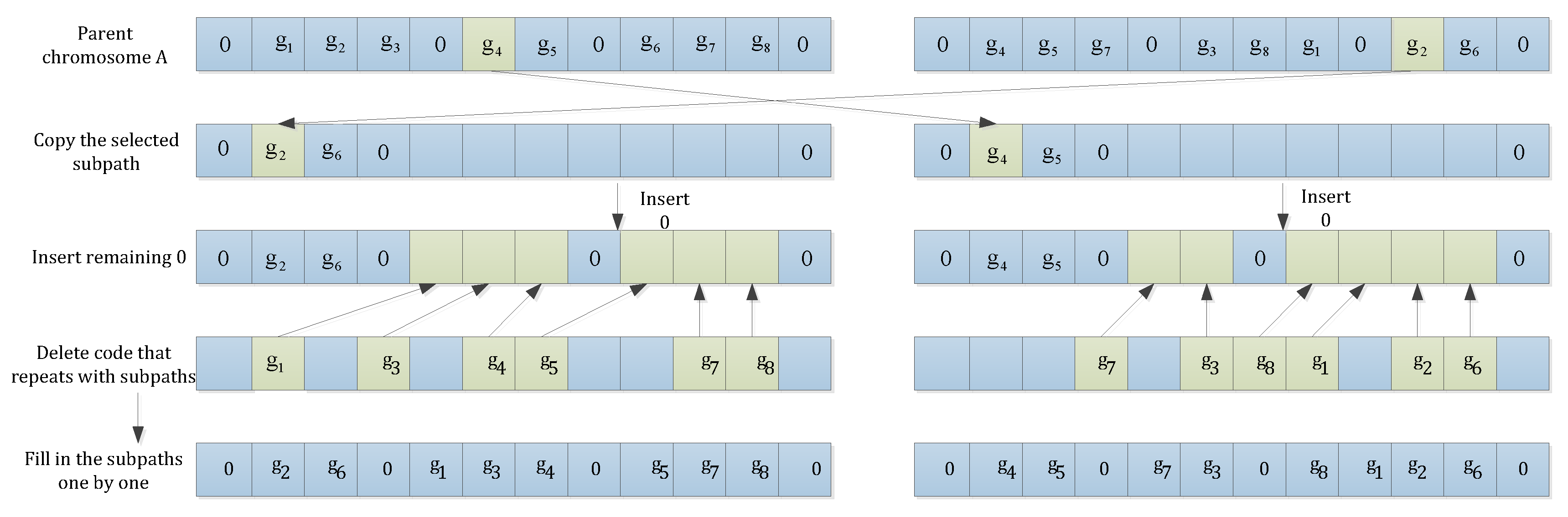
4.5. Selection, Crossover, and Mutation Operators

(1) Selection operator: The fitness values calculated by the fitness function are sorted, and individuals with higher fitness are selected and copied to the next generation. In this paper, the proportion selection method is adopted to pass on individuals with higher fitness to the next population with greater probability. Generally, the randomness of proportional selection may lead to the algorithm falling into a local optimum. For this reason, combining the simulated annealing and genetic algorithms can not only avoid too slow a convergence speed, but can also help the algorithm escape from the local optimum.

(2) Crossover operator: In this paper, we adopt partial matching crossover to achieve the purpose of optimization. Chromosome coding in the algorithm has the characteristics of intergroup disorder and intragroup order. The traditional crossover method can destroy good chromosome fragments, and no new individuals can be produced when two parents are the same. Selecting the distribution center (numbered 0) as the crossover location in the chromosome code string, we do not simply copy the substring, but move it to the first place during the crossing process, to protect the excellent chromosome fragments. The detailed operation is shown in Figure 4.

(3) Mutation operator: The mutation operator can accelerate the convergence speed of the algorithm, which improves the local search ability, avoids losing the opportunity to find the optimal solution, maintains the diversity of the population, and prevents premature phenomena. Chromosomes are randomly selected with a probability of 0.05 and two natural numbers $t_i$ and $t_j$ are randomly generated in the range $\left[1,n+m\right]$. The two numbers (denoting gene codes) are crossed to produce new individuals. If the generated numbers correspond to zero genes, it needs to regenerate. The specific operation is shown in Figure 5.

4.6. Termination Conditions

When the annealing temperature reaches the set minimum value or the current optimal solution remains unchanged for many times, the algorithm terminates and the optimal result is obtained. If the algorithm reaches the set maximum number of iterations or the population is not in the evolution, the entire operation is terminated, and the specific scheme and delivery cost of the optimal vehicle transportation obtained by this iteration are displayed.

5. Simulation Experiment and Result Analysis

5.1. Description of Instance and Experimental Environment

In order to verify the superiority of the algorithm proposed in this paper, partial data in the benchmark instance A-n37-k5 were used to test it, and sensitivity analysis of the variation of preference value $\alpha$ was performed. The model and algorithm presented in this paper were verified by simulation analysis performed on classical Solomon benchmarks, and the improved hybrid algorithm was compared with the standard simulated annealing algorithm and genetic algorithm.

The running software platform of this algorithm was the MATLAB 2018b integrated development environment in Windows 10, and the hardware platform was a computer with an Intel Core i5-8250 CPU and 8 GB RAM (The equipment is made by Huawei in Chengdu of China). The initial population was set to 300, the vehicle load was 500, the fixed cost of each vehicle was 100, and the unit transportation cost of the vehicle was 10. After many experiments, the crossover probability was set to 0.9, the mutation probability was 0.05, and the penalty fee was related to the total cost of the route.

5.2. Experiment in a Sample Instance

The A-n37-k5 instance has 37 customers, from which the first 30 items were selected for a demonstration. The first data item, number 1, represents the distribution center, and its coordinates are [38, 46], and the others represent 29 customers. Detailed information of the 29 customers is shown in

Table 2. Detailed information of nodes.

No.	x	y	Demand	No.	x	y	Demand
1	38	46	-----	16	36	48	5
2	59	46	16	17	45	36	16
3	96	42	18	18	73	57	7
4	47	61	1	19	10	91	4
5	26	15	13	20	98	51	22
6	66	6	8	21	92	62	7
7	96	23	23	22	43	43	23
8	37	25	7	23	53	25	16
9	68	92	27	24	78	65	2
10	78	84	1	25	72	79	2
11	82	28	3	26	37	88	9
12	93	90	6	27	16	73	2
13	74	42	24	28	75	96	12
14	60	20	19	29	11	66	1
15	78	58	2	30	9	49	9

.

The important parameters used in this experiment were as follows: The maximum number of iterations was 300, and the maximum number of unchanged current optimal solutions was 20. The crossover probability was 0.9 and the mutation probability was 0.05 in the GA. The fixed cost per vehicle was 100 and the variable cost per mile was 10. Under the condition that other parameters remained constant, preference value $\alpha$ increased from 0.1 to 1.0 gradually, and the average values obtained by the algorithm running 10 times are reported in

Table 3. Impact of variable $\alpha$ on costs.

A	Route Cost	Time Cost	Penalty Cost	Total Cost
0.1	3165.33	89.75	255.45	4351.15
0.2	3246.54	90.61	257.63	4339.37
0.3	3209.71	88.98	256.92	4277.83
0.4	3193.26	89.25	258.77	4196.46
0.5	3006.09	88.64	260.55	4138.41
0.6	3227.15	89.79	257.39	4375.34
0.7	3421.48	90.53	260.93	4299.71
0.8	3568.9	91.62	265.47	4239.53
0.9	3504.11	92.88	278.36	4447.68
1	3732.27	93.58	279.49	4585.27

.

The total cost consists of penalty cost, time cost, and route cost. As can be seen from Table 3, with the gradual increase in preference value $\alpha$ (i.e., slowly growing risk awareness of decision-makers), the punishment cost of distribution vehicle residual loads not satisfying customer demand also increases, which suggests that decision-makers have to pay a higher punishment cost when they judge that the remaining vehicle load is not enough to complete the current distribution task. In addition, when preference value $\alpha$ gradually increases from 0.1 to 0.5, the distribution, time, and total cost of the vehicle decrease little by little. Further, as preference value $\alpha$ increases from 0.5 to 1.0, those three costs gradually increase, showing a V-shape trend. Thus, it is reasonable to set preference value $\alpha$ to 0.5 or so in real operations.

5.3. Comparative Analysis of Algorithms

In order to verify the effectiveness of the model proposed in this paper, 10 instances with and without time window constraints modified from the Solomon 50 benchmarks were utilized to test the delivery costs for comparison. Preference value $\alpha =0.5$ was selected according to the analysis above, and other parameters were kept constant. The results reported in

Table 4. Cost comparison of instances with and without soft time windows.

e.g.,	With Soft Time Windows			Without Soft Time Windows
	k	Time Cost	Total Cost	k	Time Cost	Total Cost
C101	3	90.75	4277.01	3	73.35	4369.54
C102	3	88.61	4283.68	3	72.64	4354.27
C103	2	90.98	4159.93	2	77.58	4342.85
C104	4	87.25	4319.72	2	78.52	4521.33
C105	2	91.64	4124.55	3	68.63	4238.76
C106	3	88.79	4305.72	3	73.22	4395.04
C107	3	88.53	4211.4	2	77.83	4321.78
C108	2	90.62	4199.23	2	76.42	4253.69
C109	3	89.88	4189.87	3	72.98	4283.47
C201	3	90.58	4423.27	3	73.57	4498.06

were obtained by the algorithm running 10 times on average.

As can be seen from Table 4, due to the constraint of soft time windows, the time cost of vehicles in the whole distribution process significantly increases, but the total cost significantly decreases, which indicates that this constraint improves the overall efficiency of the logistics distribution network. At the same time, the time cost is relatively low in the case of a large number of vehicles, because increasing the number of vehicles can increase the probability of satisfying the customer’s time window and thus reducing the time cost, but this will lead to an increase in the fixed cost of vehicles.

In order to make a fair comparison, we still chose the 10 instances mentioned above to validate the hybrid algorithm proposed in this paper. The combined population genetic algorithm and genetic simulated annealing algorithm was adopted for comparison. Here, we set the maximum iterations to 200. The experimental results are shown in

Table 5. Performance comparison.

e.g.,	Optimal		Dual Population Genetic Algorithm			Genetic Simulated Annealing Algorithm			SA-GA
	k	Total Cost	k	Total Cost	Gap (%)	k	Total Cost	Gap (%)	k	Total Cost	Gap (%)
C101	3	4279.16	2	4380.68	2.41	3	4332.15	1.21	3	4279.16	0
C102	3	4146.58	3	4200.95	1.22	2	4146.58	0	3	4159.93	0.23
C103	2	4397.38	3	4431.01	0.78	3	4421.06	0.55	2	4397.38	0
C104	3	4428.58	3	4428.58	0	3	4521.13	2.09	2	4435.04	0.13
C105	2	4138.29	3	4188.96	1.25	2	4231.57	2.25	2	4138.29	0
C106	3	4438.54	3	4487.92	1.13	3	4438.54	0	2	4455.34	0.36
C107	2	4199.23	2	4276.13	1.84	3	4243.11	1.04	2	4199.23	0
C108	3	4189.86	3	4198.17	0.24	3	4288.55	2.37	3	4189.86	0
C109	3	4423.26	3	4538.06	2.61	3	4526.23	2.3	3	4423.26	0
C201	3	4685.27	3	4761.73	1.65	3	4695.19	0.3	3	4685.27	0

.

It can be seen from Table 5 that the average results obtained by the hybrid algorithm proposed in this paper can basically reach the optimal solution. Among the 10 instances, only 3 fail to obtain the optimal solution, but the error between them is within 0.4%. It can be clearly seen from the other data that the results of the hybrid algorithm are better than those of the combined population genetic algorithm and genetic simulated annealing algorithm. At the same time, using two vehicles in half of the instances can meet the distribution demand, which indicates that the hybrid algorithm proposed in this paper can arrange fewer vehicles to reach the lowest cost consumption.

6. Conclusions and Future Works

In view of uncertain customer demand in the distribution process, this paper proposes a fuzzy demand vehicle routing problem with soft time windows and insufficient demand constraints. A model with minimal total cost is established based on credibility measure theory, adding soft time windows, and imposing an additional penalty cost to deal with delivery failures when the demand cannot be satisfied. The hybrid SA-GA is designed by combining the genetic algorithm with the simulated annealing algorithm. The simulated annealing algorithm controls the convergence of the algorithm to avoid falling into the local optimal solution. The two algorithms are combined to form a parallel genetic simulated annealing algorithm. The combination of the two algorithms improves the evolutionary ability, optimization performance, and search ability. Through analyzing a large number of experiments, we can make the following conclusions:

(1) A model based on the reliability measure is established, which further deepens and expands the research on VRPFD and VRPFDFTW. The model fully considers the uncertainty information existing in reality, is closer to the actual situation encountered in vehicle distribution, and can effectively solve the problem.

(2) The fuzziness of the customer service time window can not only reduce the number of vehicles used based on ensuring customer satisfaction, but also shorten the driving distance of vehicles, thereby reducing the cost of enterprise distribution.

(3) The hybrid SA-GA has a stronger optimization capability than the two algorithms independently and can effectively escape from the local optimum.

Future work could be carried out based on the following three aspects:

(1) The running time of the program is greatly increased (about 2–3 times that of the classical genetic algorithm) because the algorithm designed in this paper combines simulated annealing and genetic algorithms. In the future, distributed computing could be used to further accelerate the running speed.

(2) The customer locations used in the instances were known in advance, so adding stochastic customers to the model would make it closer to the actual application.

(3) The same algorithm framework achieved by different programmers could lead to diverse results, so improvement and innovation of the classic algorithm are ongoing.

References

1. Wang, J.; Li, B. Multi-objective tabu search algorithm for vehicle routing problem with fuzzy due-time. Comput. Integr. Manuf. Syst. 2011, 17, 858–866. [Google Scholar]
2. Hoogeboom, M.; Dullaert, W.; Lai, D.; Vigo, D. Efficient neighborhood evaluations for the vehicle routing problem with multiple time windows. Transp. Sci. 2020, 54, 400–416. [Google Scholar] [CrossRef]
3. Kuo, R.J.; Wibowo, B.S.; Zulvia, F.E. Application of a fuzzy ant colony system to solve the dynamic vehicle routing problem with uncertain service time. Appl. Math. Model. 2016, 40, 9990–10001. [Google Scholar] [CrossRef]
4. Nadizadeh, A.; Hosseini, N.H. Solving the dynamic capacitated location-routing problem with fuzzy demands by hybrid heuristic algorithm. Eur. J. Oper. Res. 2014, 238, 458–470. [Google Scholar] [CrossRef]
5. Li, Y.; Fan, H.M.; Zhang, X.N.; Yang, X. Two-phase variable neighborhood tabu search for the capacitated vehicle routing problem with fuzzy demand. Syst. Eng. Theory Pract. 2018, 38, 522–531. [Google Scholar]
6. Zhang, X.N.; Fan, H.M. Optimization for multi-trip vehicle routing problem with fuzzy demands considering time window preference. Comput. Integr. Manuf. Syst. 2018, 10, 2461–2477. [Google Scholar]
7. Lei, H.; Laporte, G.; Guo, B. The capacitated vehicle routing problem with stochastic demands and time windows. Comput. Oper. Res. 2011, 38, 1775–1783. [Google Scholar] [CrossRef]
8. Ferreira, H.S.; Bogue, E.T.; Noronha, T.F. Variable neighborhood search for vehicle routing problem with multiple time windows. Electron. Notes Discret. Math. 2018, 66, 207–214. [Google Scholar] [CrossRef]
9. Qi, M.Y.; Zhang, J.J.; Ren, L. Vehicle routing algorithm based on spatiotemporal clustering. Comput. Sci. 2014, 41, 218–222. [Google Scholar]
10. Amiri-Aref, M.; Javadian, N.; Tavakkoli-Moghaddam, R.; Baboli, A.; Shiripour, S. The center location-dependent relocation problem with a probabilistic line barrier. Appl. Soft Comput. 2013, 13, 3380–3391. [Google Scholar] [CrossRef]
11. Alizadeh, M.; Mahdavi, I.; Mahdavi-Amiri, N.; Shiripour, S. A capacitated location-allocation problem with stochastic demands using sub-sources: An empirical study. Appl. Soft Comput. 2015, 34, 551–571. [Google Scholar] [CrossRef]
12. Shiripour, S.; Mahdavi-Amiri, N. Optimal distribution of the injured in a multi-type transportation network with damage-dependent travel times: Two metaheuristic approaches. Socio Econ. Plan. Sci. 2018, 68, 100660. [Google Scholar] [CrossRef]
13. Shen, L.; Tao, F.; Wang, S. Multi-depot open vehicle routing problem with time windows based on carbon trading. Int. J. Environ. Res. Public Health 2018, 15, 2025. [Google Scholar] [CrossRef] [PubMed] [Green Version]
14. Shi, Y.; Lv, L.; Hu, F.; Han, Q. A heuristic solution method for multi-depot vehicle routing-based waste collection problems. Appl. Sci. 2020, 10, 2403. [Google Scholar] [CrossRef] [Green Version]
15. Wang, Z.; Zhou, C.Y. A three-stage saving-based heuristic for vehicle routing problem with time windows and stochastic travel timesa. Discret. Dyn. Nat. Soc. 2016, 2016, 7841297. [Google Scholar] [CrossRef] [Green Version]
16. Yang, J.; Sun, H. Battery swap station location-routing problem with capacitated electric vehicles. Comput. Oper. Res. 2015, 55, 217–232. [Google Scholar] [CrossRef]
17. Shiripour, S.; Mahdavi-Amiri, N.; Mahdavi, I. Optimal location-multi-allocation-routing in capacitated transportation networks under population-dependent travel times. Int. J. Comput. Integr. Manuf. 2015, 29, 652–676. [Google Scholar] [CrossRef]
18. Shiripour, S.; Mahdavi-Amiri, N.; Mahdavi, I. A transportation network model with intelligent probabilistic travel times and two hybrid algorithms. Transp. Lett. 2017, 9, 90–122. [Google Scholar] [CrossRef]
Figure 1. Illustration of distribution routes: (a) is a normal distribution route and (b) is a distribution route with replenishment.
Sustainability 14 05658 g001
Figure 2. Relationship between customer satisfaction and time window.
Sustainability 14 05658 g002
Figure 3. Hybrid SA-GA framework.
Sustainability 14 05658 g003
Figure 4. Example of crossover operation.
Sustainability 14 05658 g004
Figure 5. Illustration of mutation operation.
Sustainability 14 05658 g005